Comments on “Particle Markov Chain Monte Carlo” by C. Andrieu, A. Doucet and R. Hollenstein

Abstract

We merge in this note our two discussions about the Read Paper “Particle Markov chain Monte Carlo” (Andrieu, Doucet, and Holenstein, 2010) presented on October 16^th 2009 at the Royal Statistical Society, appearing in the Journal of the Royal Statistical Society Series B. We also present a more detailed version of the ABC extension.

1 Introduction

The article Andrieu et al. (2010) is clearly going to have significant impact on scientific disciplines with a strong interface with computational statistics and non-linear state space models. Our comments are based on practical experience with PMCMC implementation in latent process multifactor SDE models for commodities (Peters et al., 2009), wireless communications (Nevat et al., 2009) and population dynamics (Hayes et al., 2009), using Rao-Blackwellised particle filters (Doucet et al., 2000) and adaptive MCMC (Roberts and Rosenthal, 2009).

2 Generic comments

• From our implementations, ideal use cases consist of highly non-linear dynamic equations for a small dimension $d_{x}$ of the state-space, large dimension $d_{\theta}$ of the static parameter, and potentially large length $T$ of the time series. In our cases $d_{x}$ was $2$ or $3$, $d_{\theta}$ up to $20$, and $T$ between $100$ and $400$.

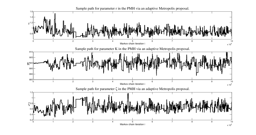
• In PMH, non-adaptive MCMC proposals for $\theta$ (e.g. tuned according to pre-simulation chains or burn-in iterations) would be costly for large $T$, and requires to keep $N$ fixed over the whole run of the Markov chain. Adaptive MCMC proposals such as the Adaptive Metropolis sampler (Roberts and Rosenthal, 2009), avoid such issues and proved particularly relevant for large $d_{\theta}$ and $T$, as can be seen in Figure 2.

• The Particle Gibbs (PG) could potentially stay frozen on a state $x_{1:T}(i)$. Consider a state space model with state transition function almost linear in $x_{n}$ for some range of $\theta$, from which $y_{1:T}$ is considered to result, and strongly non-linear elsewhere. If the PG samples $\theta(i)$ in those regions of strong non-linearity, the particle tree would likely coalesce on the trajectory preserved by the conditional SMC, leaving it with a high importance weight, maintaining $(\theta(i+1),x_{1:T}(i+1))=(\theta(i),x_{1:T}(i))$ over several iterations. Using PMH within PG would help escape this region, especially using PRC and adaptive SMC kernels, outlined in another comment, to fight the degeneracy of the filter and the high variance of $\hat{p}_{\theta}(y_{1:T})$.

3 Adaptive Sequential Monte Carlo

Our comments on adaptive SMC relate to Particle marginal Metropolis-Hastings (PMMH) which has acceptance probability given in Equation (13) of the read paper for proposed state $\left(\theta^{\ast},X^{\ast}_{1:T}\right)$, relying on the estimate $\hat{p}_{\theta^{\ast}}\left(y_{1:T}\right)=\displaystyle\prod_{n=1}^{T}\frac{1}{N}\sum_{k=1}^{N}w_{n}\left(x_{1:n}^{\ast,k}\right)$. Although a small $N$ suffices to approximate the mode of joint path space distribution, producing a reasonable proposal for $x_{1:T}$, it results in high variance estimates of $\hat{p}_{\theta^{\ast}}\left(y_{1:T}\right)$. We study a population dynamics example from (Hayes et al., 2009, Model 3 excerpt), involving a log-transformed theta-logistic state space model, see (Wang, 2007, Equation 3(a), 3(b)) for parameter settings. PMCMC performance depends on the trade-off between degeneracy of the filter, $N$, and design of the SMC mutation kernel. Regarding the latter:

• A Rao-Blackwellised filter (Doucet et al., 2000) can improve acceptance rates, Nevat et al. (see 2009).

• Adaptive mutation kernels, which in PMCMC, can be considered as adaptive SMC proposals, can reduce degeneracy on the path space, allowing for higher dimensional state vectors $x_{n}$. Adaption can be local (within filter) or global (sampled Markov chain history). Though currently particularly designed for ABC methods, the work of Peters et al. (2008) incorporates into the mutation kernel of SMC Samplers (Del Moral et al., 2006) the Partial Rejection Control (PRC) mechanism of Liu (2001), which is also beneficial for PMCMC. PRC adaption reduces degeneracy by rejecting a particle mutation when its incremental importance weight is below a threshold $c_{n}$. The PRC mutation kernel

  $$q_{\theta}^{\ast}(x_{n}|y_{n},x_{n-1})=r(c_{n},x_{n-1})^{-1}\min\left[1,W_{n-1}(x_{n-1})\frac{w_{n}(x_{n-1},x_{n})}{c_{n}}\right]q_{\theta}(x_{n}|y_{n},x_{n-1}),$$ (1)

  can also be used in PMH, where $q_{\theta}(x_{n}|y_{n},x_{n-1})$ is the standard SMC proposal, and

  $$r(c_{n},x_{n-1})=\int\min\left[1,W_{n-1}(x_{n-1})\frac{w_{n}(x_{n-1},x_{n})}{c_{n}}\right]q_{\theta}(x_{n}|y_{n},x_{n-1})dx_{n}.$$ (2)

  As presented in Peters et al. (2008), algorithmic choices for $q_{\theta}^{\ast}(x_{n}|y_{n},x_{n-1})$ can avoid evaluation of $r(c_{n},x_{n-1})$. Cornebise (2009b) extend this work, developing PRC for Auxiliary SMC samplers, also useful in PMH. Threshold $c_{n}$ can be set adaptively: locally either at each SMC mutation or Markov chain iteration; or globally based on chain acceptance rates. Additionally, $c_{n}$ can be set adaptively via quantile estimates of pre-PRC incremental weights, see Peters et al. (2009).

• Cornebise et al. (2008) state that adaptive SMC proposals can be designed by minimizing function-free risk theoretic criteria such as Kullback-Leibler divergence between a joint proposal in a parametric family and a joint target. Cornebise (2009a, Chapter 5) and Cornebise et al. (2009) use a mixture of experts, adapting kernels of a mixture on distinct regions of the state-space separated by a softmax partition. These results extend to PMCMC settings.

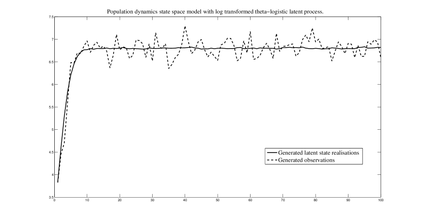
Figure 1: Sequence of simulated states and observations for the population dynamic log-transformed theta logistic model from Wang (2007), with static parameter $\theta=(r,\zeta,K)$ under constraints $K>0$, $r<2.69$, $\zeta\in\mathbb{R}$. State transition is $f_{\theta}(x_{n}|x_{n-1})=\mathcal{N}\left(x_{n};x_{n-1}+r\left(1-(\exp(x_{t-1})/K)^{\zeta}\right),0.01\right)$, and local likelihood is $g_{\theta}(y_{n}|x_{n})=\mathcal{N}\left(y_{n};x_{n},0.04\right)$, for $T=100$ timesteps.

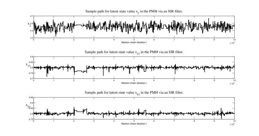
Figure 2: Path of three sampled latent states $x_{2}$, $x_{37}$, $x_{93}$, and of the sampled parameters $\theta=(r,\zeta,L)$, over $100,000$ PMH iterations based on $N=200$ particles using a simple SIR filter – the one dimensional state did not call for Rao-Blackwellisation. Note also the effect the Adaptive MCMC proposal for $\theta$, set-up to start at iteration $5,000$, particularly visible on the mixing of parameter $K$. The most noticeable property of the algorithm is the remarkable mixing of the chain, in spite of the high total dimension of the sampled state: each iteration involves a proposal of $(X_{1:T},\theta)$ of dimension $103$.

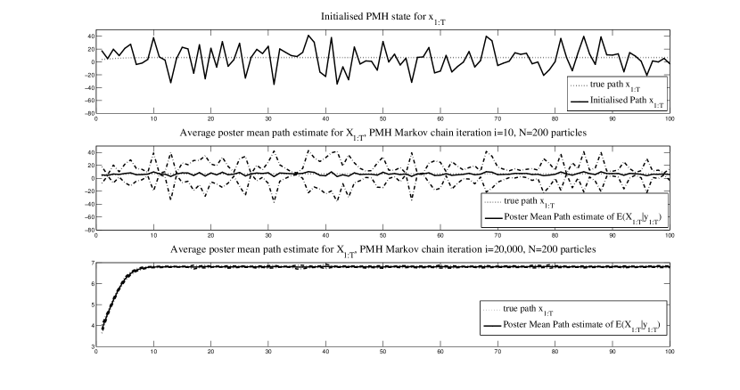
Figure 3: Convergence of the distribution of the path of latent states $x_{1:T}$. Note the change of vertical scale. Initializing PMH on a very unlikely initial path does not prevent the MMSE estimate of the latent states converging: as few as $10$ PMH iterations already begins to concentrate the sampled paths around the true path – assumed here to be close to the mode of the posterior distribution thanks to the small observation noise –, with very satisfactory results after $20,000$ iterations.

4 Approximate Bayesian Computation and PMCMC

For intractable joint likelihood $p_{\theta}(y_{1:T}|x_{1:T})$, we could design a SMC-ABC algorithm (see e.g. Peters et al., 2008; Ratmann, 2010, Chapter 1) for a fixed ABC tolerance $\epsilon$, using the approximations

$$\hat{p}^{ABC}_{\theta}\left(y_{1:T}\right):=\frac{1}{N}\sum_{k=1}^{N}\frac{\frac{1}{S}\sum_{s=1}^{S}\mathbb{I}\left(\rho(y^{k}_{1}(s),y_{1})<\epsilon\right)\mu_{\theta}(x^{k}_{1})}{q_{\theta}(x^{k}_{1}|y_{1})}\\ \times\prod_{n=2}^{T}\left(\frac{1}{N}\sum_{k=1}^{N}\frac{\frac{1}{S}\sum_{s=1}^{S}\mathbb{I}\left(\rho(y^{k}_{n}(s),y_{n})<\epsilon\right)f_{\theta}(x^{k}_{n}|x^{A^{k}_{n-1}}_{n-1})}{q_{\theta}(x^{k}_{n}|y_{n},x^{A^{k}_{n-1}}_{n-1})}\right)$$

or

$$\hat{p}^{ABC}_{\theta}\left(y_{1:T}\right):=\frac{1}{N}\sum_{k=1}^{N}\frac{\frac{1}{S}\sum_{s=1}^{S}\mathcal{N}\left(y^{k}_{1}(s);y_{1},\epsilon^{2}\right)\mu_{\theta}(x^{k}_{1})}{q_{\theta}(x^{k}_{1}|y_{1})}\\ \times\prod_{n=2}^{T}\left(\frac{1}{N}\sum_{k=1}^{N}\frac{\frac{1}{S}\sum_{s=1}^{S}\mathcal{N}\left(y^{k}_{n}(s);y_{n},\epsilon^{2}\right)f_{\theta}(x^{k}_{n}|x^{A^{k}_{n-1}}_{n-1})}{q_{\theta}(x^{k}_{n}|y_{n},x^{A^{k}_{n-1}}_{n-1})}\right)$$

with $\rho$ a distance on the observation space and $y^{k}_{n}(s)\sim g_{\theta}(\cdot|x^{k}_{n})$ simulated observations. Additional degeneracy on the path space induced by ABC approximation should be controlled, e.g. with PRC (Peters et al., 2008), see Equation (1). More details on this algorithm are available in Appendix A, which is not contained in our comment to JRSSB due to space restrictions.

Appendix A Algorithmic details of ABC filtering within PMCMC

Algorithm 1 SMC-ABC-PRC filtering algorithm targeting $p_{\theta}(x_{1:T}|y_{1:T})$ as required in Step 2(b) of the PMMH of (Andrieu et al., 2010, Section 2.4.2). Replaces the SMC algorithm presented in (Andrieu et al., 2010, Section 2.2.1). Approximation $g_{\theta}^{ABC}$ is defined in Equation (3) and function $r$ in Equation (2).

1. Initialize $\epsilon$ and $c_{1}$

2. At time $n=1$,

   1. for $k=1,\ldots,N$

      1. sample $X^{k}_{1}\sim q_{\theta}(\cdot|y_{1})$

      2. sample $Y_{1}^{k}(s)\sim g_{\theta}(\cdot|X^{k}_{1})$ for $s=1,\ldots,S$

      3. compute the incremental weight

         $$\tilde{w}_{1}(X^{k}_{1}):=\frac{\mu_{\theta}(X^{k}_{1})g_{\theta}^{ABC}(y_{1}|X^{k}_{1},Y_{1}^{k}(1\!\!:\!\!S),\epsilon)}{q_{\theta}(X^{k}_{1}|y_{1})}\;,$$

      4. with probability $1-p^{k}_{1}=1-\min\{1,\tilde{w}_{1}(X^{k}_{1})/c_{1}\}$, reject $X^{k}_{1}$ and go to (i)

      5. otherwise, accept $X^{k}_{1}$ and set

         $$w_{1}(X^{k}_{1})=\tilde{w}_{1}(X^{k}_{1})r(c_{1})/p^{k}_{1}$$

   2. normalise the weights $W_{1}^{k}:=w_{1}(X^{k}_{1})/\sum_{m=1}^{N}w_{1}(X^{m}_{1})$.

3. At times $n=2,\ldots,T$,

   1. possibly adapt $c_{n}$ online

   2. for $k=1,\ldots,N$

      1. sample $A^{k}_{n-1}\sim\mathcal{F}(\cdot|\mathbf{W}_{n-1})$,

      2. sample $X^{k}_{n}\sim q_{\theta}(\cdot|y_{n},X^{A^{k}_{n-1}}_{n-1})$ and set $X^{k}_{1:n}=(X^{A^{k}_{n-1}}_{n-1},X^{k}_{n})$, and

      3. sample $Y_{n}^{k}(s)\sim g_{\theta}(\cdot|X^{k}_{n})$ for $s=1,\ldots,S$

      4. compute the incremental weight

         $$\tilde{w}_{n}(X^{k}_{1:n}):=\frac{f_{\theta}(X^{k}_{n}|X^{A^{k}_{n-1}}_{n-1})g_{\theta}^{ABC}(y_{n}|X^{k}_{n},Y_{n}^{k}(1\!\!:\!\!S),\epsilon)}{q_{\theta}(X^{k}_{n}|y_{n},X^{A^{k}_{n-1}}_{n-1})}\;,$$

      5. with probability $1-p^{k}_{n}=1-\min\{1,\tilde{w}_{n}(X^{k}_{1:n})/c_{n}\}$, reject $X^{k}_{n}$ and go to (ii)

      6. otherwise, accept $X^{k}_{n}$ and set

         $$w_{n}(X^{k}_{1:n})=\tilde{w}_{n}(X^{k}_{1:n})r(c_{n},X^{A^{k}_{n-1}}_{n-1})/p^{k}_{n}$$

   3. normalise the weights $W_{n}^{k}:=w_{n}(X^{k}_{1:n})/\sum_{m=1}^{N}w_{n}(X^{m}_{1:n})$.

Here we expand on the comment we made above in which we approximated the local likelihood $g_{\theta}(y_{n}|x_{n})$ of the SMC-based filtering part of the PMCMC algorithm. by the ABC approximation

$$g_{\theta}^{ABC}(y_{n}|x_{n},y_{n}(1\!\!:\!\!S),\epsilon):=\frac{1}{S}\sum_{s=1}^{S}\pi_{\theta}\left(y_{n}(s)|x_{n},y_{n},\epsilon\right)$$ (3)

where possible choices for $\pi_{\theta}$ are

$$\pi^{\mathbb{I}}_{\theta}\left(y_{n}(s)|x_{n},y_{n},\epsilon\right):=\mathbb{I}\left(\rho(y_{n}(s),y_{n})<\epsilon\right)\text{ or }\pi^{\mathcal{N}}_{\theta}\left(y_{n}(s)|x_{n},y_{n},\epsilon\right):=\mathcal{N}\left(y_{n}(s);y_{n},\epsilon^{2}\right)$$

with $\rho$ a distance on the observation space and $y_{n}(s)\sim g_{\theta}(\cdot|x_{n})$ simulated observations – assumed here to be univariate for sake of brevity, but generalisation to multivariate setting and summary statistics is straightforward.

We note it is critical in the filtering context to ensure that the particle system under approximation does not collapse into uniformly null incremental weights $w_{n}\left(X^{k}_{1:n}\right)=0$ which may occur for $\pi^{\mathbb{I}}_{\theta}$ at any stage of the filtering during each PMCMC iteration, especially for small tollerances $\epsilon$. The PRC mutation kernel $q^{\ast}_{\theta}(x_{n}|y_{n},x_{n-1})$ defined in Equation (1) is critical to overcome both this collapse and the additional degeneracy on the path space introduced by the ABC approximation. The algorithm presented in McKinley et al. (2009, Sections 3.4 and 3.5.1) is a special case of the SMC samplers PRC-ABC algorithm of Peters et al. (2008) in which the PRC rejection threshold $c_{n}=0$, the mutation kernel is global and resampling is performed at each stage of the filter, which avoids the computation of the normalizing constant $r(c_{n},x_{n-1})$ defined in Equation (2). We further note that the work of Cornebise (2009a) casts the SMC sampler PRC algorithm (Peters et al., 2008) with rejection of the ancestor index $A^{k}_{n-1}$ – here in Step 3.(a).(v) – into an Auxiliary SMC sampler framework. The combination of these two concepts recovers a generalized version of McKinley et al. (2009), see Algorithm 1, which has advantage in the PMCMC setting of allowing for adaptation of the threshold $c_{n}$.

References

• Andrieu et al. (2010) Andrieu, C., A. Doucet, and R. Holenstein (2010). Particle Markov chain Monte Carlo methods. J. R. Statis. Soc. B 72(2), 1–33.
• Cornebise (2009a) Cornebise, J. (2009a). Adaptive Sequential Monte Carlo Methods. Ph. D. thesis, University Pierre and Marie Curie – Paris 6.
• Cornebise (2009b) Cornebise, J. (2009b). Auxiliary SMC samplers with applications to PRC and ABC. Working paper, Stastistical and Applied Mathematical Sciences Institute.
• Cornebise et al. (2008) Cornebise, J., E. Moulines, and J. Olsson (2008). Adaptive methods for sequential importance sampling with application to state space models. Statistics and Computing 18(4), 461–480.
• Cornebise et al. (2009) Cornebise, J., E. Moulines, and J. Olsson (2009). Adaptive sequential Monte Carlo by means of mixture of experts. Working paper, Telecom ParisTech.
• Del Moral et al. (2006) Del Moral, P., A. Doucet, and A. Jasra (2006). Sequential Monte Carlo samplers. Journal of the Royal Statistical Society: Series B (Statistical Methodology) 68(3), 411–436.
• Doucet et al. (2000) Doucet, A., N. de Freitas, K. Murphy, and S. Russell (2000). Rao-Blackwellised particle filtering for dynamic Bayesian networks. In Proceedings of the Sixteenth Conference on Uncertainty in Artificial Intelligence, pp.  176–183.
• Hayes et al. (2009) Hayes, K., G. Hosack, and G. Peters (2009). Searching for the allee effect in latent state space models via adaptive particle Markov chain Monte Carlo. Working paper, Department of Mathematics and Statistics, University of New South Wales.
• Liu (2001) Liu, J. (2001). Monte Carlo Strategies in Scientific Computing. New York: Springer.
• McKinley et al. (2009) McKinley, T., A. Cook, and R. Deardon (2009). Inference in epidemic models without likelihoods. The International Journal of Biostatistics 5(1), 24.
• Nevat et al. (2009) Nevat, I., G. Peters, and A. Doucet (2009). Channel tracking for relay networks via adaptive particle MCMC. Working paper, University of New South Wales.
• Peters et al. (2009) Peters, G., M. Briers, P. Shevchenko, and A. Doucet (2009). Online calibration and filtering for multi factor commodity models with seasonality: incorporating futures and options contracts. Working paper, Department of Mathematics and Statistics, University of New South Wales.
• Peters et al. (2008) Peters, G., Y. Fan, and S. Sisson (2008). On sequential Monte Carlo, partial rejection control and approximate Bayesian computation. Technical report, Department of Mathematics and Statistics, University of New South Wales.
• Peters et al. (2009) Peters, G., Y. Fan, and S. Sisson (2009). Likelihood-free Bayesian inference for α𝛼\alpha-stable models. Technical report, Department of Mathematics and Statistics, University of New South Wales.
• Ratmann (2010) Ratmann, O. (2010). Approximate Bayesian Computation under model uncertainty, with an application to stochastic processes of network evolution. Ph. D. Thesis, to appear, Imperial College.
• Roberts and Rosenthal (2009) Roberts, G. and J. Rosenthal (2009). Examples of adaptive MCMC. Journal of Computational and Graphical Statistics 18(2), 349–367.
• Wang (2007) Wang, G. (2007). On the latent state estimation of nonlinear population dynamics using bayesian and non-Bayesian state-space models. Ecological Modelling 200(3-4), 521–528.