Convergent Interpolation to Cauchy Integrals over Analytic Arcs with Jacobi-Type Weights

Abstract.

We design convergent multipoint Padé interpolation schemes to Cauchy transforms of non-vanishing complex densities with respect to Jacobi-type weights on analytic arcs, under mild smoothness assumptions on the density. We rely on the work [9] for the choice of the interpolation points, and dwell on the Riemann-Hilbert approach to asymptotics of orthogonal polynomials introduced in [33] in the case of a segment. We also elaborate on the $\bar{\partial}$-extension of the Riemann-Hilbert technique, initiated in [37] on the line to relax analyticity assumptions. This yields strong asymptotics for the denominator polynomials of the multipoint Padé interpolants, from which convergence follows.

1. Introduction

Classical Padé approximants (or interpolants) and their multipoint generalization are probably the oldest and simplest candidate rational-approximants to a holomorphic function of one complex variable. They are simply those rational functions of type $(m,n)$ that interpolate the function in $m+n+1$ points of the domain of analyticity, counting multiplicity. Classical Padé approximants refer to the case where interpolation takes place in a single point with multiplicity $m+n+1$ [38].

Besides their everlasting number-theoretic success [43, 32, 41], they are common tools in modeling and numerical analysis of various fields, ranging from boundary value problems and convergence acceleration [16, 29, 13, 26, 20] to continuous mechanics [6, 51], quantum mechanics [8, 52], condensed matter physics [42], fluid mechanics [40], system and circuits theory [12, 31, 17], and even page ranking the Web [14].

In spite of this, the convergence properties of Padé or multipoint Padé approximants are still far from being understood. For particular classes of functions like Markov functions, some elliptic functions, and certain entire functions such as Polya frequencies or functions with smooth and fast decaying Taylor coefficients, classical Padé approximants at infinity are known to converge, locally uniformly on the domain of analyticity [36, 50, 4, 34]. But when applied to more general cases they seldom accomplish the same, due to the occurrence of “spurious poles” that may wander about the domain of analyticity. Further distinction should be made here between diagonal approximants (i.e. interpolants of type $(m,m)$) and row approximants (i.e. interpolants of type $(m,n)$ where $n$ is kept fixed), and we refer the reader to the comprehensive monograph [7] for a detailed account of many works on the subject. Let us simply mention that, for the case of diagonal approximants which is the most interesting as it treats poles and zeros on equal footing, the disproof of the Padé conjecture [35] and of the Stahl conjecture [15] have only added to the picture that classical Padé approximants are not seen best through the spectacles of uniform convergence.

The case of multipoint Padé approximants is somewhat different, since choosing the interpolation points offers new possibilities to help convergence. However, it is not immediately clear how to use these additional parameters. The theory was initially developed for Markov functions (i.e. Cauchy transforms of positive measures compactly supported on the real line) showing that multipoint Padé approximants converge locally uniformly on the complement of the smallest segment containing the support of the defining measure, provided the interpolation points are conjugate symmetric [25]. The crux of the proof is the remarkable connection between rational interpolants and orthogonal polynomials: the denominator of the $n$-th diagonal multipoint Padé approximant is the $n$-th orthogonal polynomial of the measure defining the Markov function, weighted by the inverse of the polynomial whose zeros are the interpolation points (this polynomial is identically 1 for classical Padé approximants). The conjugate symmetric distribution of the interpolation points is to the effect that the weight is positive, so one can apply the asymptotic theory of orthogonal polynomials with varying weights [49].

When trying to generalize this approach to more general Cauchy integrals than Markov functions, one is led to consider non-Hermitian orthogonal polynomials with respect to complex-valued measures on more general arcs than segments, and for a while it was unclear what could be hoped for. In the pathbreaking papers [44, 46, 47, 48], devoted to the convergence in capacity of classical Padé approximants to functions with branchpoints, it was shown that such orthogonal polynomials lend themselves to analysis when the measure is supported on a system of arcs of minimal logarithmic capacity linking the branchpoints, in the complement of which the function is single-valued. Shortly after, the same type of convergence was established for multipoint Padé approximants to Cauchy integrals of continuous (quasi-everywhere) non-vanishing densities over arcs of minimal weighted capacity, provided that the interpolation points asymptotically distribute like a measure whose potential is the logarithm of the weight [27]. Such an extremal system of arcs is called a symmetric contour, or $S$-contour, and is characterized by a symmetry property of the (two-sided) normal derivatives of its equilibrium potential. The corresponding condition on the distribution of the interpolation points may be viewed as a far-reaching generalization of the conjugate-symmetry with respect to the real line that was required to interpolate Markov functions in a convergent way.

After these works it became apparent that the appropriate class of Cauchy integrals for Padé approximation should consist of those taken over $S$-contours, and that the interpolation points should distribute according to the weight that defines the symmetry property. However, it is not so easy to decide which systems of arcs are $S$-contours, since finding a weight making the arcs of smallest weighted capacity is a nontrivial inverse problem, and in any case convergence in capacity is much weaker than locally uniform convergence.

For the class of Jordan arcs, new ground was recently broken in [9] where it is shown that such an arc, if rectifiable and Ahlfors regular at the endpoints, is an $S$-contour if and only if it is analytic. The proof recasts the $S$-property for Jordan arcs as the existence of a sequence of “pseudo-rational” functions, holomorphic and tending to zero off the arc, whose boundary values from each side of the latter remain bounded, and whose zeros remain at positive distance from the arc. There are in fact many such sequences that can be computed explicitly from an analytic parameterization of the arc. Then, translating the non-Hermitian orthogonality equation for the denominator into an integral equation involving Hankel operators and using compactness properties of the latter, the reference just quoted establishes that multipoint Padé approximants to Cauchy transforms of Dini-continuous (essentially) non-vanishing densities with respect to the equilibrium distribution of the arc converge locally uniformly in its complement when the interpolation points are the zeros of these pseudo-rational functions.

Still the above result remains unsatisfactory, for the hypotheses entail that the density with respect to arclength in the integral goes to infinity towards the endpoints of the arc, since so does the equilibrium distribution. In particular, ultra-smooth situations like the one of Cauchy integrals of smooth functions over analytic arcs are not covered. The present paper develops a new technique to handle any non-vanishing integrable Jacobi-type density under mild smoothness assumptions, thereby settling more or less the issue of convergence in multipoint Padé interpolation to functions defined as Cauchy integrals over analytic Jordan arcs.

We dwell on the Riemann-Hilbert approach to asymptotics of orthogonal polynomials with analytic weights, pioneered on the line in [11, 19] and carried over to the segment in [33]. We also elaborate on the $\bar{\partial}$-extension thereof, initiated on the line in [37] to relax the analyticity requirement. This will provide us with strong (i.e. Plancherel-Rotach type) asymptotics for the denominator polynomials of the multipoint Padé interpolants we construct and for their associated functions of the second kind, from which the local uniform convergence we seek follows easily. It is interesting to note that the Riemann-Hilbert approach, which is typically a tool to obtain sharp quantitative asymptotics, is here used as a means to solve a qualitative question namely the convergence of the interpolants.

The interpolation points shall be the same as in [9], namely the zeros of a sequence of pseudo-rational functions adapted to the arc. Such an interpolation scheme will prove convergent for all Cauchy integrals with sufficiently smooth density with respect to a Jacobi weight on the arc at the same time. This provides us with a varying weight which is not of power type, nor in general converging sufficiently fast to a weight of power type to take advantage of the results of [3], where the Riemann-Hilbert approach is adapted to non-Hermitian orthogonality with analytic weights on smooth $S$-arcs. Instead, when “opening the lens”, we set up a sequence of Riemann-Hilbert problems with varying contours whose solutions converge to the desired one by properties of the pseudo rational functions.

We pay special attention to keep smoothness requirements low, in order to obtain as general a result as the method permits. Roughly speaking, the higher the Jacobi exponents the smoother the density should be, see the precise assumptions (2.9). When the Jacobi exponents are negative, only a fraction of a derivative is needed, which compares not too badly with the Dini-continuity assumption in [9]. In the present setting, however, the density cannot vanish whereas some weak vanishing is still allowed in [9]. We are of course rewarded here with stronger asymptotics.

As the varying part of our weight is analytic, the extension inside the lens with controlled $\bar{\partial}$-estimates, introduced in [37] for power weights, needs only deal with the density defining the Cauchy integral we interpolate. This step is treated using either tools from real analysis, e.g. Muckenhoupt weights and Sobolev traces, or else classical Hölder estimates for singular integrals, whichever yields the best results granted the Jacobi exponents.

Since we consider analytic arcs only, it is natural to ask how general our results with respect to the general class of Cauchy integrals over rectifiable Jordan arcs. It turns out that they are as general as can be, because if the Cauchy integral of a nontrivial Jacobi weight can be interpolated in a convergent way with a triangular scheme of interpolation points that stay away from the arc, then the arc is in fact analytic [10].

The paper is organized as follows. Section 2 fixes notation and defines pseudo rational functions as well as multipoint Padé approximants before stating the main results. In Section 3, the contours that will later be instrumental for the solution of the Riemann-Hilbert problem are introduced. Section 4 contains preliminaries on smooth extensions from boundary data in domains with polygonal boundaries. Section 5 is devoted to key estimates of certain singular integral operators that play a main role in the extension of the weight. Section 6 and 7 deal with the analytic Riemann-Hilbert problem, while Section 8 solves the $\overline{\partial}$ version thereof. Finally, in Section 9, we gather the material developed so far to establish the asymptotics and the convergence of multipoint Padé approximants stated in Section 2.

2. Statements of Results

Let $\Delta$ be a closed analytic Jordan arc with endpoints $-1$ and $1$. That is to say, there exists a holomorphic univalent function $\Xi$, defined in some domain $D_{\Xi}\supset[-1,1]$, such that

$$\Delta=\Xi([-1,1]),\quad\Xi(\pm 1)=\pm 1.$$

We call $\Xi$ an analytic parameterization of $\Delta$. We orient $\Delta$ from $-1$ to $1$ and, according to this orientation, we distinguish the left and the right sides of $\Delta$ denoted by $\Delta^{+}$ and $\Delta^{-}$, respectively. It will be convenient to introduce two unbounded arcs, say, $\Delta_{l}$ and $\Delta_{r}$, that respectively connect $-\infty$ to $-1$ and 1 to $+\infty$, in such a manner that $\Delta_{l}\cup\Delta\cup\Delta_{r}$ is a smooth unbounded Jordan arc that coincides with the real line in some neighborhood of infinity. Define on $\Delta$ the Jacobi weight

(2.1) $$w(z)=w(\alpha,\beta;z):=(1-z)^{\alpha}(1+z)^{\beta},\quad\alpha,\beta>-1,$$

where we choose branches of $(1-z)^{\alpha}$ and $(1+z)^{\beta}$ that are holomorphic outside of $\Delta_{r}$ and $\Delta_{l}$, respectively, and assume value 1 at the origin. In particular, $w$ is analytic across $\Delta^{\circ}:=\Delta\setminus\{\pm 1\}$. Further, set

(2.2) $$\mathfrak{w}(z):=\sqrt{z^{2}-1},\quad\mathfrak{w}(z)/z\to 1,\quad\mbox{as}\quad z\to\infty,$$

to be a holomorphic branch of the square root outside of $\Delta$. Then

(2.3) $$\varphi(z):=z+\mathfrak{w}(z),\quad z\in D:=\overline{\mathbb{C}}\setminus\Delta,$$

is holomorphic in $D\setminus\{\infty\}$, has continuous boundary values $\varphi^{\pm}$ on $\Delta^{\pm}$, respectively, and satisfies

(2.4) $$\varphi^{+}\varphi^{-}=1\quad\mbox{on}\quad\Delta\quad\mbox{and}\quad\varphi(z)/2z\to 1\quad\mbox{as}\quad z\to\infty.$$

It is immediate that $\varphi$ is inverse of the Joukovski transformation $J(z):=(z^{2}+1)/2z$, i.e., $J(\varphi(z))=z$, $z\in D$. Moreover, $\varphi$ maps $D$ conformally onto an unbounded domain whose boundary is an analytic Jordan curve [9, Sec. 3.1] which is symmetric with respect to the transformation $z\mapsto 1/z$. In particular, $\varphi$ does not vanish.

2.1. Symmetric Contours

Multipoint Padé approximants to a given function $f$ are defined to be rational interpolants to $f$. In this paper we are interested in those functions $f$ that can be expressed as Cauchy integrals of Jacobi-type complex densities defined on $\Delta$ (see the smoothness assumptions in (2.8) and (2.9)). In order for multipoint Padé approximants to converge to such a function, it is necessary to choose the interpolation schemes appropriately with respect to $\Delta$. We presently characterize these schemes in terms of the associated monic polynomials vanishing at the interpolation points.

Let $\{v_{n}\}$ be a sequence polynomials such that $\deg(v_{n})\leq 2n$ and each $v_{n}$ has no zeros on $\Delta$. To this sequence we associate a sequence of “pseudo-rational” functions, say $\{r_{n}\}$, given by

(2.5) $$r_{n}(z):=\left(\frac{1}{\varphi(z)}\right)^{2n-\deg(v_{n})}\prod_{\{e:v_{n}(e)=0\}}\frac{\varphi(z)-\varphi(e)}{1-\varphi(e)\varphi(z)},\quad z\in D,$$

where the product is taken over all zeros of $v_{n}$ according to their multiplicities. It is easy to see that each function $r_{n}$ is holomorphic in $D$, has the same zeros as $v_{n}$ counting multiplicities, and vanishes at infinity with order $2n-\deg(v_{n})$. Hence, each $r_{n}$ has exactly 2n zeros counting multiplicities. Moreover, the unrestricted boundary values $r^{\pm}_{n}$ exist continuously from each side of $\Delta$ and satisfy $r^{+}_{n}r^{-}_{n}\equiv 1$ by the first part of (2.4).

Hereafter, the normalized counting measure of a finite set is the probability measure that has equal mass at each point counting multiplicities. Below, the weak^∗ topology refers to the duality between complex measures and continuous functions with compact support in $\overline{\mathbb{C}}$.

Definition 1.

We say that a sequence of polynomials $\{v_{n}\}$ with no zeros on $\Delta$ belongs to the class $\mathrm{S}(\Delta)$ if the following conditions hold:

• the associated functions $r_{n}$ via (2.5) satisfy $|r_{n}^{\pm}|=O(1)$ uniformly on $\Delta$ and $r_{n}=o(1)$ locally uniformly in $D$;

• there exists a neighborhood of $\Delta$ that contains no zeros of $r_{n}$ for all $n$ large enough;

• the normalized counting measures of zeros of $r_{n}$ form a weak^∗ convergent sequence.

The third requirement in the definition of $\mathrm{S}(\Delta)$ is purely technical and is placed only to simplify the forthcoming considerations since one can always proceed with subsequences as far as convergence is concerned.

Regarding the nature of the class $\mathrm{S}(\Delta)$, the following result was obtained in [9, Thm. 1]. For a closed analytic Jordan arc $\Delta$, there always exist sequences $\{v_{n}\}$ belonging to $\mathrm{S}(\Delta)$ and they can be constructed explicitly granted the parameterization $\Xi$. A partial converse is also true. Namely, let $\Delta$ be a rectifiable Jordan arc with endpoint $\pm 1$ such that for $x=\pm 1$ and all $t\in\Delta$ sufficiently close to $x$ it holds that $|\Delta_{t,x}|\leq\textnormal{const.}|x-t|^{\beta}$, $\beta>1/2$, where $|\Delta_{t,x}|$ is the length of the subarc of $\Delta$ joining $t$ and $x$ and “const.” is an absolute constant. If there exists a sequence of polynomials $\{v_{n}\}$ meeting the first two requirements of Definition 1, then $\Delta$ is necessarily analytic. The class $\mathrm{S}(\Delta)$ is also intimately related to the so-called symmetry property of the contour $\Delta$ [44, 45, 9].

For our investigation we need to detail further the properties of the just defined interpolation schemes. We gather them in the following theorem. We agree that the arcs involved have endpoints $\pm 1$. Moreover, we say that two holomorphic functions are analytic continuations of each other if they are defined on domains that have nonempty intersection on which the functions coincide.

Theorem 1.

Let $\Delta$ be a closed analytic Jordan arc and $\{v_{n}\}\in\mathrm{S}(\Delta)$. Then there exists a sequence of closed analytic Jordan arcs $\{\Delta_{n}\}$ such that:

• there exist analytic parametrizations $\Xi_{n}$ of $\Delta_{n}$ and $\Xi$ of $\Delta$ such that the functions $\Xi_{n}$ converge to $\Xi$ uniformly in some neighborhood of $[-1,1]$ as $n\to\infty$;

• for each function $r_{n}$, associated to $v_{n}$ via (2.5), there exists an analytic continuation $r_{n}^{*}$, holomorphic in $D_{n}:=\overline{\mathbb{C}}\setminus\Delta_{n}$, such that $|(r_{n}^{*})^{\pm}|\equiv 1$ on $\Delta_{n}$.

Let $\mathfrak{w}_{n}$ and $\varphi_{n}$ be defined relative to $\Delta_{n}$ as $\mathfrak{w}$ and $\varphi$ were defined in (2.2) and (2.3) relative to $\Delta$. Clearly, $\mathfrak{w}_{n}$ and $\varphi_{n}$ are analytic continuations of $\mathfrak{w}$ and $\varphi$ to $D_{n}$. In fact, $r_{n}^{*}$ is simply the function associated to $v_{n}$ via (2.5) with $\varphi$ replaced by $\varphi_{n}$. It is apparent that $r_{n}^{*}$ is nothing but the Blaschke product with respect to $D_{n}$ that has the same zeros as $r_{n}$.

2.2. Multipoint Padé Approximation

Let $\mu$ be a complex Borel measure with compact support. We define the Cauchy transform of $\mu$ as

(2.6) $$f_{\mu}(z):=\int\frac{d\mu(t)}{z-t},\quad z\in\overline{\mathbb{C}}\setminus\textnormal{supp}(\mu).$$

Clearly, $f_{\mu}$ is a holomorphic function in $\overline{\mathbb{C}}\setminus\textnormal{supp}(\mu)$ that vanishes at infinity.

Classically, diagonal (multipoint) Padé approximants to $f_{\mu}$ are rational functions of type $(n,n)$ that interpolate $f_{\mu}$ at a prescribed system of $2n+1$ points. However, when the approximated function is of the from (2.6), it is customary to place at least one interpolation point at infinity so as to let the approximants vanish at infinity as well by construction.

Definition 2.

Let $f_{\mu}$ be given by (2.6) and $\{v_{n}\}$ be a sequence of monic polynomials, $\deg(v_{n})\leq 2n$, with zeros in $\overline{\mathbb{C}}\setminus\textnormal{supp}(\mu)$. The $n$-th diagonal Padé approximant to $f_{\mu}$ associated with $\{v_{n}\}$ is the unique rational function $\Pi_{n}=p_{n}/q_{n}$ satisfying:

• $\deg p_{n}\leq n$, $\deg q_{n}\leq n$, and $q_{n}\not\equiv 0$;

• $\left(q_{n}(z)f_{\mu}(z)-p_{n}(z)\right)/v_{n}(z)$ is analytic in $\overline{\mathbb{C}}\setminus\textnormal{supp}(\mu)$;

• $\left(q_{n}(z)f_{\mu}(z)-p_{n}(z)\right)/v_{n}(z)=O\left(1/z^{n+1}\right)$ as $z\to\infty$.

A multipoint Padé approximant always exists since the conditions for $p_{n}$ and $q_{n}$ amount to solving a system of $2n+1$ homogeneous linear equations with $2n+2$ unknown coefficients, no solution of which can be such that $q_{n}\equiv 0$ (we may thus assume that $q_{n}$ is monic); note that the required interpolation at infinity is entailed by the last condition and therefore $\Pi_{n}$ is, in fact, of type $(n-1,n)$.

We consider only absolutely continuous measures that are supported on $\Delta$ and whose densities are Jacobi weights (2.1) multiplied by suitably smooth non-vanishing functions. This leads us to define smoothness classes $\mathrm{C}^{m,\varsigma}$.

Definition 3.

Let $K$ be an infinitely smooth closed Jordan arc or curve. We say that $\theta\in\mathrm{C}^{m,\varsigma}(K)$ if $\theta$ is $m$-times continuously differentiable on $K$ with respect to the arclength and its $m$-th derivative is uniformly Hölder continuous with exponent $\varsigma$, i.e.,

$$|\theta^{(m)}(t_{1})-\theta^{(m)}(t_{2})|\leq\textnormal{const.}|t_{1}-t_{2}|^{\varsigma},\quad t_{1},t_{2}\in K.$$

When $K=\Delta$, we simply write $\mathrm{C}^{m,\varsigma}$ instead of $\mathrm{C}^{m,\varsigma}(\Delta)$. We also write $\mathrm{C}^{\infty}(K)$ for the space of infinitely differentiable functions on $K$.

Together with $\mathrm{C}^{m,\varsigma}$, we also consider fractional Sobolev spaces.

Definition 4.

Let $K$ be an infinitely smooth Jordan arc or curve. We say that $\theta\in\mathrm{W}^{1-1/p}_{p}(K)$, $p\in(1,\infty)$, if

$$\iint_{K\times K}\left|\frac{\theta(x)-\theta(y)}{x-y}\right|^{p}|dx||dy|<\infty.$$

When $K=\Delta$, we simply write $\mathrm{W}^{1-1/p}_{p}$ instead of $\mathrm{W}^{1-1/p}_{p}(K)$.

We shall be interested only in the case $p\in(2,\infty)$ since in this range it holds that

(2.7) $$\mathrm{W}_{p}^{1-1/p}\subset\mathrm{C}^{0,\varsigma},\quad\varsigma=1-\frac{2}{p},\quad p\in(2,\infty).$$

by Sobolev imbedding theorem (see Section 4.1).

In what follows, we assume that the measure $\mu$ in (2.6) is of the form

(2.8) $$d\mu(t)=(wh)(t)dt,\quad h(t)=e^{\theta(t)},\quad t\in\Delta,$$

where the Jacobi weight $w=w(\alpha,\beta;\cdot)$ and the complex function $\theta$ are such that

(2.9) $$\alpha,\beta\in(-s,s)\cap(-1,\infty)$$

with

$$s:=\left\{\begin{array}[]{lll}1-\frac{2}{p},&\mbox{if}\quad\theta\in\mathrm{W}_{p}^{1-1/p},&p\in(2,\infty),\vskip 3.0pt plus 1.0pt minus 1.0pt\\ 2\varsigma-1,&\mbox{if}\quad\theta\in\mathrm{C}^{0,\varsigma},&\varsigma\in\left(\frac{1}{2},1\right],\vskip 3.0pt plus 1.0pt minus 1.0pt\\ m+\varsigma,&\mbox{if}\quad\theta\in\mathrm{C}^{m,\varsigma},&m\in\mathbb{N},\quad\varsigma\in(0,1].\end{array}\right.$$

To describe the asymptotic behavior of the approximation error to functions $f_{\mu}$ by the multipoint Padé approximants, we need to introduce complex geometric means and Szegő functions. The geometric mean of $h=e^{\theta}$ is given by

(2.10) $$G_{h}:=\exp\left\{\int\theta d\omega\right\},\quad d\omega(t):={\frac{idt}{\pi\mathfrak{w}^{+}(t)}},\quad t\in\Delta.$$

The measure $\omega$ is, in some sense, natural for the considered problem as suggested by the forthcoming Theorem 2. Observe also that $\omega$ simply becomes the normalized arcsine distribution on $\Delta$ when $\Delta=[-1,1]$. As $\int d\omega=1$, $G_{h}$ depends only on $h$ and is non-zero when $\theta$ is Hölder continuous (see Section 5.3). Moreover, in this case the Szegő function of $h$, given by

(2.11) $$S_{h}(z):=\exp\left\{\frac{\mathfrak{w}(z)}{2}\int\frac{\theta(t)}{z-t}d\omega(t)-\frac{1}{2}\int\theta d\omega\right\},\quad z\in D,$$

is the unique non-vanishing holomorphic function in $D$ that has continuous unrestricted boundary values on $\Delta$ from each side and satisfies

(2.12) $$h=G_{h}S_{h}^{+}S_{h}^{-}\quad\mbox{on}\quad\Delta\quad\mbox{and}\quad S_{h}(\infty)=1.$$

The main result of the paper is the following theorem.

Theorem 2.

Let $\Delta$ be a closed analytic Jordan arc connecting $\pm 1$ and $\{v_{n}\}\in\mathrm{S}(\Delta)$. Let also $f_{\mu}$ a Cauchy integral (2.6) with $\mu$ given by (2.8) and (2.9). Then $\{\Pi_{n}\}$, the sequence of diagonal multipoint Padé approximants to $f_{\mu}$ associated with $\{v_{n}\}$, is such that

$$(f_{\mu}-\Pi_{n})\mathfrak{w}=\left[2G_{\dot{\mu}}+o(1)\right]S^{2}_{\dot{\mu}}\;r_{n},$$

with $o(1)$ satisfying

(2.13) $$|o(1)|\leq\frac{\textnormal{const.}}{n^{a}},\quad a\in\left\{\begin{array}[]{ll}\left(0,\frac{s-\max\{|\alpha|,|\beta|\}}{2}\right),&s-\max\{|\alpha|,|\beta|\}\leq 1,\vskip 3.0pt plus 1.0pt minus 1.0pt\\ \left(0,\frac{1}{2}\right),&s-\max\{|\alpha|,|\beta|\}>1,\end{array}\right.$$

locally uniformly in $D$, where the constant const. depends on $a$, $d\mu=\dot{\mu}d\omega$, i.e., $\dot{\mu}=-i\pi wh\mathfrak{w}^{+}$, and the functions $r_{n}$ are associated to the polynomials $v_{n}$ via (2.5) and hence converge to zero geometrically fast in $D$.

The convergence theory of Padé approximants to Cauchy integrals is strongly interwoven with asymptotic behavior of underlying orthogonal polynomials that are the denominators of $\Pi_{n}$. In fact, it is easy to show that $f_{\mu}-\Pi_{n}=R_{n}/q_{n}$, where $R_{n}$ is a function associated to $q_{n}$ via (2.15), and $q_{n}$ satisfies the orthogonality relations of the form (2.14), (2.16) (see, for example, [9, Thm. 4]). Hence, Theorem 2 follows from Theorem 3 below.

2.3. Strong Asymptotics for non-Hermitian Orthogonal Polynomials

In this section we investigate the asymptotic behavior of polynomials satisfying non-Hermitian orthogonality relations of the form

(2.14) $$\int_{\Delta}t^{j}q_{n}(t)w_{n}(t)dt=0,\quad j\in\{0,\ldots,n-1\},$$

together with the asymptotic behavior of their functions of the second kind, i.e.,

(2.15) $$R_{n}(z):=R_{n}(q_{n};z)=\int_{\Delta}\frac{q_{n}(t)w_{n}(t)}{t-z}\frac{dt}{\pi i},\quad z\in D,$$

where $\{w_{n}\}$ is the sequence of varying weights specified in (2.16).

Theorem 3.

Let $\{q_{n}\}$, $\deg(q_{n})\leq n$, be a sequence of polynomials satisfying orthogonality relations (2.14) with weights given by

(2.16) $$w_{n}:=\frac{wh_{n}h}{v_{n}},\quad h=e^{\theta},\quad h_{n}=e^{\theta_{n}},$$

where $\theta$ and $w=w(\alpha,\beta;\cdot)$ are as in (2.9), $\{\theta_{n}\}$ is a normal family in some neighborhood of $\Delta$, and $\{v_{n}\}\in\mathrm{S}(\Delta)$. Then, for all $n$ large enough, the polynomials $q_{n}$ have exact degree $n$ and therefore can be normalized to be monic. Under such a normalization, we have that

(2.17) $$\left\{\begin{array}[]{lll}q_{n}&=&[1+o(1)]/S_{n}\vskip 3.0pt plus 1.0pt minus 1.0pt\\ R_{n}\mathfrak{w}&=&[1+o(1)]\gamma_{n}S_{n}\end{array}\right.$$

with $o(1)$ satsfying (2.13) locally uniformly in $D$, where

(2.18) $$S_{n}:=(2/\varphi)^{n}S_{w_{n}\mathfrak{w}^{+}},\quad\gamma_{n}:=2^{1-2n}G_{w_{n}\mathfrak{w}^{+}},$$

and $R_{n}$ was defined in (2.15). Moreover, it holds that

(2.19) $$\left\{\begin{array}[]{lll}q_{n}&=&[1+o(1)]/S_{n}^{+}+[1+o(1)]/S_{n}^{-}\vskip 3.0pt plus 1.0pt minus 1.0pt\\ (R_{n}\mathfrak{w})^{\pm}&=&[1+o(1)]~{}\gamma_{n}S_{n}^{\pm}\end{array}\right.,$$

where $o(1)$ satisfies (2.13) locally uniformly in $\Delta^{\circ}$.

The method of proof can also be used to derive the asymptotics of $q_{n}$ and $R_{n}$ around $\pm 1$ as was done in [33]. However, the corresponding calculations are lengthy and do not impinge on the convergence of Padé interpolants proper, which is why the authors decided to omit them here.

The appearance of the normal family $\{\theta_{n}\}$ in (2.16) is not necessitated by Theorem 2 but is included for possible application to meromorphic approximation [53].

3. Proof of Theorem 1 and $g$-Functions

In this section we prove Theorem 1. The notion of $g$-function, which we introduce along the way, will be needed later on for the proof of Theorem 3.

3.1. Parameterization $\Xi$, functions $g$ and $\widetilde{g}$

Let $\{v_{n}\}\in\mathrm{S}(\Delta)$ and $r_{n}$ be associated to $v_{n}$ by (2.5). As required by Definition 1-(2) and (3), the normalized counting measures of the zeros of $r_{n}$ converge weak^∗ to a Borel measure $\nu$, $\textnormal{supp}(\nu)\subset D$. Denote by $V_{D}^{\nu}$ the Green potential of this measure with respect to $D$. It was shown in the course of the proof of [9, Thm. 1, see (4.34)] that Definition 1-(1) yields

(3.1) $$V_{D}^{\nu}(z)=-\int\log\left|\frac{\varphi(z)-\varphi(t)}{1-\varphi(z)\varphi(t)}\right|d\nu(t).$$

In other words, the Green kernel $-\log\left|\frac{\phi(z)-\phi(t)}{1-\overline{\phi(t)}\phi(z)}\right|$, where $\phi$ is the conformal map of $D$ onto $\{|z|>1\}$ such that $\phi(\infty)=\infty$ and $\phi^{\prime}(\infty)>0$, can be replaced by the one in (3.1) for this special measure $\nu$.

The Green potential $V_{D}^{\nu}$ is a positive harmonic function in $D\setminus\textnormal{supp}(\nu)$ whose boundary values vanish everywhere on $\Delta$. Let $L_{\rho}:=\{z:~{}V_{D}^{\nu}(z)=\log\rho\}$, $\rho>1$, be a level line of $V_{D}^{\nu}$ in $\Xi(D_{\Xi})$, the range of $\Xi$. Without loss of generality we may assume that $\rho$ is a regular value and therefore $L_{\rho}$ is a smooth Jordan curve encompassing $\Delta=L_{1}$. Denote by $O$ the domain bounded by $L_{\rho}$ and $\Delta$. Set

(3.2) $$\partial f:=\frac{1}{2}\left(\partial_{x}f-i\partial_{y}f\right)\quad\mbox{and}\quad\bar{\partial}f:=\frac{1}{2}\left(\partial_{x}f+i\partial_{y}f\right).$$

Since $\nu$ is a probability measure, it can be verified as in the proof of [9, Thm. 1, see (4.39) and after] that the function

(3.3) $$\Phi(z):=\exp\left\{2\int_{1}^{z}\frac{\partial V_{D}^{\nu}}{\partial z}(t)dt\right\}=\exp\left\{-\int\log\frac{\varphi(z)-\varphi(t)}{1-\varphi(z)\varphi(t)}d\nu(t)\right\}$$

is well-defined in $O$ and maps it conformally onto the annulus $\{z:~{}1<|z|<\rho\}$ while $\Phi(\pm 1)=\pm 1$, where we take any path from $1$ to $z$ contained in $O\setminus\Delta$. Moreover, by direct examination of the kernel in (3.3), we get that

(3.4) $$\Phi^{+}=\overline{\Phi^{-}}=1/\Phi^{-}\quad\mbox{on}\quad\Delta.$$

This, in particular, yields that $J\circ\Phi$ is holomorphic across $\Delta$, where $J(z)=(z+1/z)/2$ is the Joukovski transformation. Consequently, the inverse $(J\circ\Phi)^{-1}$ is a holomorphic univalent map in some neighborhood of $[-1,1]$ that analytically parametrizes $\Delta$. In what follows, we assume that $\Xi=(J\circ\Phi)^{-1}$.

Based on the conformal map $\Phi$, we define two more functions, $g$ and $\widetilde{g}$ as follows. Set $L:=\Phi^{-1}([-\rho,-1])$, $\widetilde{L}:=\Phi^{-1}([1,\rho])$ (see Fig. 1), and define

(3.5) $$\begin{array}[]{lll}g:=\log\Phi,&\displaystyle\lim_{z\to 1}g(z)=0,&g\in\mathrm{H}(O\setminus L),\vskip 3.0pt plus 1.0pt minus 1.0pt\\ \widetilde{g}:=\log\Phi-\pi i,&\displaystyle\lim_{z\to-1}\widetilde{g}(z)=0,&\widetilde{g}\in\mathrm{H}(O\setminus\widetilde{L}).\end{array}$$

It follows immediately from (3.4) that

(3.6) $$g^{+}=-g^{-}\quad\mbox{and}\quad\widetilde{g}^{+}=-\widetilde{g}^{-}\quad\mbox{on}\quad\Delta.$$

Hence, $g^{2}$ and $\widetilde{g}^{2}$ are analytic in $O_{g}:=(O\cup\Delta)\setminus L$ and $O_{\widetilde{g}}:=(O\cup\Delta)\setminus\widetilde{L}$, respectively. Moreover, it holds that $g^{2}(\Delta)=\widetilde{g}^{2}(\Delta)=[-\pi^{2},0]$ and $g^{2}(1)=\widetilde{g}^{2}(-1)=0$. It is also true that $g^{2}$ and $\widetilde{g}^{2}$ are univalent in $O_{g}$ and $O_{\widetilde{g}}$, respectively. Indeed, suppose that $g^{2}(z_{1})=g^{2}(z_{2})$, $z_{1},z_{2}\in O_{g}$. Then either $\Phi(z_{1})=\Phi(z_{2})$ and therefore $z_{1}=z_{2}$ by conformality of $\Phi$ or $\Phi(z_{1})=1/\Phi(z_{2})$, which is possible only if $\Phi^{+}(z_{1})=\overline{\Phi^{-}(z_{2})}$, i.e., if $z_{1}=z_{2}\in\Delta$. The case of $\widetilde{g}^{2}$ is no different.

3.2. Jordan arcs $\Delta_{n}$, functions $g_{n}$ and $\widetilde{g}_{n}$

By Definition 1-(2) and upon taking $\rho$ smaller if necessary, we may assume that functions $r_{n}$ have no zeros in $\overline{O}$. Moreover, as $r_{n}$ is holomorphic in $D\setminus\Delta$ and has $2n$ zeros in $D\setminus\overline{O}$, its winding number is equal to $-2n$ on any positively oriented curve homologous to $L_{\rho}$ and contained in $O$. In other words, $r_{n}$ has a continuous argument that decreases by $4n\pi$ as $\Delta$ is encompassed once in the positive direction. Thus, the functions

$$\Phi_{n}:=r_{n}^{-1/2n}=\exp\left\{-\int\log\frac{\varphi(z)-\varphi(t)}{1-\varphi(z)\varphi(t)}d\nu_{n}(t)\right\},$$

are well-defined and analytic in $O$, where $\nu_{n}$ is the normalized counting measure of the zeros of $r_{n}$. Moreover, as the counting measures of zeros of $r_{n}$ converge weak^∗ to $\nu$ by assumption, the functions $\Phi_{n}$ converge to $\Phi$ uniformly in $\overline{O}$, distinguishing the one-sided values on $\Delta^{\pm}$.

Hence, we can define

(3.7) $$\begin{array}[]{lll}g_{n}:=\log\Phi_{n},&\displaystyle\lim_{z\to 1}g_{n}(z)=0,&g_{n}\in\mathrm{H}(O\setminus L),\vskip 3.0pt plus 1.0pt minus 1.0pt\\ \widetilde{g}_{n}:=\log\Phi_{n}-\pi i,&\displaystyle\lim_{z\to-1}\widetilde{g}_{n}(z)=0,&\widetilde{g}_{n}\in\mathrm{H}(O\setminus\widetilde{L}).\end{array}$$

By (2.4), it is straightforward to see that $\Phi_{n}^{+}\Phi_{n}^{-}\equiv 1$ on $\Delta$, and therefore

(3.8) $$g_{n}^{+}=-g_{n}^{-}\quad\mbox{and}\quad\widetilde{g}_{n}^{+}=-\widetilde{g}_{n}^{-}\quad\mbox{on}\quad\Delta.$$

Thus, $g_{n}^{2}$ and $\widetilde{g}_{n}^{2}$ are analytic in $O_{g}$ and $O_{\widetilde{g}}$, respectively. We choose domains $O_{L}\subset O_{g}$ and $O_{\widetilde{L}}\subset O_{\widetilde{g}}$ in such a manner that $O_{L}\supset\widetilde{L}$, $O_{\widetilde{L}}\supset L$, and $O_{L}\cup O_{\widetilde{L}}$ is simply connected and contains $\Delta$ (see Fig. 1). Then it is an easy consequence of the convergence of $\Phi_{n}$ to $\Phi$ that $g_{n}^{2}$ and $\widetilde{g}_{n}^{2}$ converge uniformly to $g^{2}$ and $\widetilde{g}^{2}$ on $\overline{O}_{L}$ and $\overline{O}_{\widetilde{L}}$, respectively.

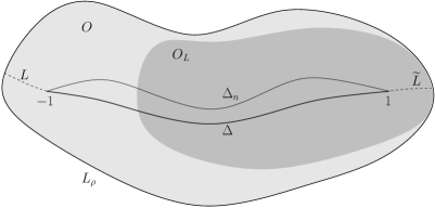
Figure 1. The domain $O$ bounded by $\Delta$ and $L_{\rho}$(light grey), the domain $O_{L}\subset O\cup\Delta$ (dark grey), the cuts $L$ and $\widetilde{L}$ (dashed arcs).

Next, we claim that $g_{n}^{2}$ and $\widetilde{g}_{n}^{2}$ are univalent for all $n$ large enough in $\overline{O}_{L}$ and $\overline{O}_{\widetilde{L}}$, respectively. Assume to the contrary that there exist two sequences of points $\{z_{1,n}\},\{z_{2,n}\}\subset\overline{O}_{L}$ such that $g_{n}^{2}(z_{1,n})=g_{n}^{2}(z_{2,n})$. As $\overline{O}_{L}$ is compact, we can assume that $z_{j,n}\to z_{j}\in\overline{O}_{L}$, $j=1,2$. Since $g_{n}^{2}$ converges to $g^{2}$ uniformly on $\overline{O}_{L}$, we have that $g^{2}(z_{1})=g^{2}(z_{2})$ and therefore $z_{1}=z_{2}$. Set $d_{n}(z):=(g^{2}_{n}(z)-g^{2}_{n}(z_{1,n}))/(z-z_{1,n})$. Then $d_{n}$ are analytic functions on $\overline{O}_{L}$ that converge uniformly to $d(z):=(g^{2}(z)-g^{2}(z_{1}))/(z-z_{1})$. Moreover, the values $d_{n}(z_{2,n})$ are equal to $0$ and converge to $d(z_{1})$. Thus, $(g^{2})^{\prime}(z_{1})=d(z_{1})=0$, which is impossible since $g^{2}$ is univalent. This proves the claim as the case of $\widetilde{g}_{n}^{2}$ is no different.

From the above we see that each $g_{n}^{2}$ maps $O_{L}$ conformally onto a neighborhood of zero as $g_{n}^{2}(1)=0$. Set $\Delta_{n,1}$ to be the preimage of the intersection of this neighborhood with $\Sigma_{2}:=\{\zeta:~{}\textnormal{Arg}(\zeta)=\pi\}$. Then $\Delta_{n,1}$ is an analytic arc with one endpoint being 1. Analogously, $\widetilde{g}_{n}^{2}$ maps $O_{\widetilde{L}}$ conformally into another neighborhood of zero. Thus, we can define $\Delta_{n,-1}$ to be again the preimage of the intersection of this neighborhood with $\Sigma_{2}$. Clearly, $\Delta_{n,-1}$ is an analytic arc with one endpoint being $-1$. Noticing that $g_{n}^{2}$ assumes negative values if and only if $\widetilde{g}_{n}^{2}$ assumes negative values on the common set of definition $O_{L}\cap O_{\widetilde{L}}$, we derive that $\Delta_{n}:=\Delta_{n,1}\cup\Delta_{n,-1}$ is an analytic arc with endpoint $\pm 1$.

3.3. Parameterizations $\Xi_{n}$, functions $g_{n}^{*}$ and $\widetilde{g}_{n}^{*}$

Now, define $\mathfrak{w}_{n}$ and $\varphi_{n}$ with respect to $\Delta_{n}$ like $\mathfrak{w}$ and $\varphi$ were defined in (2.2) and (2.3) with respect to $\Delta$. Clearly, $\varphi_{n}$ is an analytic continuation of $\varphi$ from $D$ onto $D_{n}=\overline{\mathbb{C}}\setminus\Delta_{n}$. Further, let $r_{n}^{*}$ be defined by (2.5) with $\varphi$ replaced by $\varphi_{n}$ while keeping the same zeros as $r_{n}$. Hence, $r_{n}^{*}$ and $r_{n}$ are analytic continuations of each other defined in $D$ and $D_{n}$, respectively. Finally, set $\Phi_{n}^{*}$, $g_{n}^{*}$, and $\widetilde{g}_{n}^{*}$ to be the analytic continuations of $\Phi_{n}$, $g_{n}$, and $\widetilde{g}_{n}$ from $O$, $O\setminus L$, and $O\setminus\widetilde{L}$, onto $O_{n}:=(O\cup\Delta)\setminus\Delta_{n}$, $O_{n}\setminus L$, and $O_{n}\setminus\widetilde{L}$, defined in, by now, obvious manner. Hence

$$g_{n}^{2}=(g_{n}^{*})^{2}\quad\mbox{and}\quad\widetilde{g}_{n}^{2}=(\widetilde{g}_{n}^{*})^{2},$$

while $(g_{n}^{*})^{2}$ is negative on $\Delta_{n}$. Since, in addition, $(g_{n}^{*})^{+}=-(g_{n}^{*})^{-}$ on $\Delta_{n}$, $(g_{n}^{*})^{\pm}$ are pure imaginary on $\Delta_{n}$ and $|\Phi_{n}^{*}|\equiv 1$ there. Therefore, $(\Phi_{n}^{*})^{+}=\overline{(\Phi_{n}^{*})^{-}}$ and $(r_{n}^{*})^{+}=\overline{(r_{n}^{*})^{-}}$. Furthermore, $\Phi_{n}^{*}$ maps $O_{n}$ onto some annular domain having the unit circle as a component of its boundary. Arguing as was done after (3.4), we derive that $J\circ\Phi_{n}^{*}$ is holomorphic across $\Delta_{n}$ and that $\Xi_{n}:=(J\circ\Phi_{n}^{*})^{-1}$ is a holomorphic parameterization of $\Delta_{n}$, $\Xi_{n}([-1,1])=\Delta_{n}$. Moreover, as the functions $\Phi_{n}$ converge to $\Phi$ uniformly in some annular domain encompassing $\Delta$, we see that the functions $J\circ\Phi_{n}^{*}$ converge locally uniformly to $J\circ\Phi$ in some neighborhood of $\Delta$. Hence, the sequence of analytic parameterizations $\{\Xi_{n}\}$ of $\Delta_{n}$ converges uniformly to the analytic parameterization $\Xi$ of $\Delta$ in some neighborhood of $[-1,1]$. This finishes the proof of Theorem 1.

4. Trace Theorems and Extensions

As is usual in the Riemann-Hilbert approach to asymptotics of orthogonal polynomials, we shall need to extend the weights of orthogonality from $\Delta$ into subsets of the complex plane. As the weights are not analytic, this extension will require a special construction that we carry out in this section.

4.1. Domains with Smooth Boundaries

In this section we suppose that $\Omega$ is a bounded simply connected domain with boundary $\Gamma$ which is infinitely smooth and contains $\Delta$, i.e., $\Delta\subset\Gamma$.

Definition 5.

Set $\mathrm{L}^{p}(\Omega)$, $p\in[1,\infty)$, to be the space of all measurable functions $f$ such that $|f|^{p}$ is integrable over $\Omega$. The Sobolev space $\mathrm{W}_{p}^{1}(\Omega)$, $p\in[1,\infty)$, is the subspace of $\mathrm{L}^{p}(\Omega)$ that comprises of functions with weak partial derivatives also in $\mathrm{L}^{p}(\Omega)$.

Then the following theorem takes place [30, Thm. 1.5.1.2].

Theorem T1.

For each $f\in\mathrm{W}_{p}^{1-1/p}(\Gamma)$, $p\in(1,\infty)$, there exists $F\in\mathrm{W}_{p}^{1}(\Omega)$ such that $F_{|\Gamma}=f$. Moreover, the extension operator can be made independent of $p$. Conversely, for every $F\in\mathrm{W}^{1}_{p}(\Omega)$ it holds that $F_{|\Gamma}\in\mathrm{W}^{1-1/p}_{p}(\Gamma)$.

Together with the Sobolev spaces $\mathrm{W}_{p}^{1}(\Omega)$, we consider smoothness classes $\mathrm{C}^{m,\varsigma}(\overline{\Omega})$.

Definition 6.

By $\mathrm{C}^{m,\varsigma}(\overline{\Omega})$, $m\in\mathbb{Z}_{+}$, $\varsigma\in(0,1]$, we denote the space of all functions on $\overline{\Omega}$ whose partial derivatives up to the order $m$ are continuous on $\overline{\Omega}$ and whose partial derivatives of order $m$ are uniformly Hölder continuous on $\overline{\Omega}$ with exponent $\varsigma$. Moreover, $\mathrm{C}^{m,\varsigma}_{0}(\overline{\Omega})$ will stand for the subset of $\mathrm{C}^{m,\varsigma}(\overline{\Omega})$ consisting of functions whose partial derivatives up to order $m$, including the function itself, vanish on $\Gamma$. Finally, $\mathrm{C}^{\infty}(\overline{\Omega})$ will denote the space of functions on $\Omega$ whose partial derivatives of any order exist and are continuous on $\overline{\Omega}$.

It is known from Sobolev’s imbedding theorem [2, Thm. 5.4] that

(4.1) $$\mathrm{W}_{p}^{1}(\Omega)\subset\left\{\begin{array}[]{ll}\mathrm{L}^{2p/(2-p)}(\Omega),&p\in[1,2),\vskip 3.0pt plus 1.0pt minus 1.0pt\\ \mathrm{C}^{0,{1-2/p}}(\overline{\Omega}),&p\in(2,\infty).\end{array}\right.$$

Hence, for $f\in\mathrm{W}^{1-1/p}_{p}(\Gamma)$, $p\in(2,\infty)$, the function $F$ granted by Theorem T1 belongs to $\mathrm{C}^{0,{1-2/p}}(\overline{\Omega})$ and therefore $f\in\mathrm{C}^{0,{1-2/p}}(\Gamma)$, which is exactly what was stated in (2.7).

Later on, we shall need the following proposition.

Proposition 4.

Let $f$ be a continuous function on $\Delta$ such that $f(\pm 1)=0$. If $f\in\mathrm{W}^{1-1/p}_{p}$, $p\in(2,\infty)$, then there exists $F\in\mathrm{W}^{1}_{p}(\Omega)$ such that $F_{|\Delta}=f$. Moreover, if $f\in\mathrm{C}^{0,\varsigma}$, $\varsigma\in(1/2,1]$, then there exists $F\in\mathrm{W}^{1}_{q}(\Omega)$ for any $q\in(2,\frac{1}{1-\varsigma})$ such that $F_{|\Delta}:=f$.

Proof.

In both cases set $\tilde{f}=f$ on $\Delta$ and $\tilde{f}\equiv 0$ on $\Gamma\setminus\Delta$. When $f\in\mathrm{W}^{1-1/p}_{p}$, it is immediate to check that $\tilde{f}\in\mathrm{W}^{1-1/p}_{p}(\Gamma)$ and therefore the first claim follows from Theorem T1. When $f\in\mathrm{C}^{0,\varsigma}$, it holds that $\tilde{f}\in\mathrm{C}^{0,\varsigma}(\Gamma)$ and $\widetilde{f}\in\mathrm{W}^{1-1/q}_{q}(\Gamma)$ for any $q\in(1,\frac{1}{1-\varsigma})$ by an easy estimate (see Definition 4). Hence, the second claim of the proposition again follows from Theorem T1. ∎

To state a trace theorem for classes $\mathrm{C}^{m,\varsigma}(\overline{\Omega})$, we need to introduce the notion of a directional derivative. Namely, let $\xi$ be a continuous function on $\overline{\Omega}$ and $f\in\mathrm{W}^{1}_{p}(\Omega)$. With the slight abuse of notation, we define the derivative of $f$ in the direction of the field $\xi$, denoted by $\partial_{\xi}$, as

(4.2) $$\partial_{\xi}f:=\bar{\xi}\bar{\partial}f+\xi\partial f=\textnormal{Re}(\xi)\partial_{x}f+\textnormal{Im}(\xi)\partial_{y}f,$$

where $\nabla f$ is the gradient of $f$, $\vec{\xi}$ is the vector field with values in $\mathbb{R}^{2}$ corresponding to $\xi$.

As $\Gamma$ is infinitely smooth, any conformal map $\phi$ of $\Omega$ onto the unit disk belongs to $\mathrm{C}^{\infty}(\overline{\Omega})$ [39, Thm. 3.6]. Moreover, it holds that $\phi^{\prime}\neq 0$ in $\overline{\Omega}$. Thus, we may set

(4.3) $$n(z):=\frac{\phi(z)}{\phi^{\prime}(z)}\quad\mbox{and}\quad\mathbf{n}(z):=\phi(z)\frac{|\phi^{\prime}(z)|}{\phi^{\prime}(z)},\quad z\in\overline{\Omega}.$$

Then $n,\mathbf{n}\in\mathrm{C}^{\infty}(\overline{\Omega})$ and $n$ is holomorphic in $\Omega$. Moreover, for any $z\in\Gamma$, $\mathbf{n}(z)=n(z)/|n(z)|$ represents the complex number corresponding to the outer unit normal to $\Gamma$ at $z$. Then the following theorem takes place [30, Thm. 6.2.6].

Theorem T2(1).

Let $\{f_{k}\}_{k=0}^{m}$ be such that $f_{k}\in\mathrm{C}^{m-k,\varsigma}(\Gamma)$, $m\in\mathbb{N}$, $\varsigma\in(0,1]$, $k\in\{0,\ldots,m\}$. Then there exists $F\in\mathrm{C}^{m,\varsigma}(\overline{\Omega})$ such that $(\partial_{\mathbf{n}}^{k}F)_{|\Gamma}=f_{k}$, $k\in\{0,\ldots,m\}$.

Now, observe that

$$\partial^{k}_{\mathbf{n}}=|\phi^{\prime}|^{k}\partial^{k}_{n}+\sum_{j=1}^{k-1}c_{k,j}\partial^{j}_{n},$$

where the functions $c_{k,j}$ involve sums and products of the powers of the iterated directional derivatives of $|\phi^{\prime}|$ with respect to the field $n$ and therefore belong to $\mathrm{C}^{\infty}(\overline{\Omega})$. Set $c_{k,k}:=|\phi^{\prime}|^{k}$ and $c_{k,j}\equiv 0$, $j\in\{k+1,\ldots,m\}$, $k\in\{1,\ldots,m\}$. Then the matrix $\mathscr{C}_{\phi}=[c_{k,j}]_{k,j=1}^{m}$ is such that $\det(\mathscr{C}_{\phi})=|\phi^{\prime}|^{m(m+1)/2}$, which is non-vanishing at any $z\in\overline{\mathbb{C}}$, and

$$(\partial_{\mathbf{n}},\ldots,\partial^{m}_{\mathbf{n}})^{\mathrm{T}}=\mathscr{C}_{\phi}(\partial_{n},\ldots,\partial^{m}_{n})^{\mathrm{T}}.$$

Thus, to every family of functions $\{f_{k}\}_{k=0}^{m}$, $f_{k}\in\mathrm{C}^{m-k,\varsigma}(\Gamma)$, there corresponds another family, say $\{\tilde{f}_{k}\}_{k=0}^{m}$, $\tilde{f}_{k}\in\mathrm{C}^{m-k,\varsigma}(\Gamma)$, such that there exists $F\in\mathrm{C}^{m,\varsigma}(\overline{\Omega})$ satisfying $(\partial_{\mathbf{n}}^{k}F)_{|\Gamma}=f_{k}$ and $(\partial_{n}^{k}F)_{|\Gamma}=\tilde{f}_{k}$. Moreover, this correspondence is one-to-one and onto. Hence, Theorem T2(1) can be equivalently reformulated as follows.

Theorem T2(2).

Let $\{f_{k}\}_{k=0}^{m}$ be such that $f_{k}\in\mathrm{C}^{m-k,\varsigma}(\Gamma)$, $m\in\mathbb{N}$, $\varsigma\in(0,1]$, $k\in\{0,\ldots,m\}$. Then there exists $F\in\mathrm{C}^{m,\varsigma}(\overline{\Omega})$ such that $(\partial_{n}^{k}F)_{|\Gamma}=f_{k}$, $k\in\{0,\ldots,m\}$.

Finally, we define $\tau:=in$. Clearly, $\tau(z)/|\tau(z)|$, $z\in\Gamma$, is the complex number corresponding to the positively oriented unit tangent to $\Gamma$ at $z$. Since $n$ and $\tau$ are holomorphic functions such that $\tau=in$, it is a simple computation to verify that $\partial_{n}\partial_{\tau}F=\partial_{\tau}\partial_{n}F$ in $\overline{\Omega}$. Then the following proposition holds.

Proposition 5.

Let $f\in\mathrm{C}^{m,\varsigma}(\Delta)$, $m\in\mathbb{N}$, $\varsigma\in(0,1]$, $f^{(k)}(\pm 1)=0$, $k\in\{0,\ldots,m\}$. Then there exists $F\in\mathrm{C}^{m,\varsigma}(\overline{\Omega})$ such that $F_{|\Delta}=f$ and $\bar{\partial}F\in\mathrm{C}^{m-1,\varsigma}_{0}(\overline{\Omega})$.

Proof.

Set $f_{0}=f$ on $\Delta$ and $f_{0}\equiv 0$ on $\Gamma\setminus\Delta$. It is clear that $f_{0}\in\mathrm{C}^{m,\varsigma}(\Gamma)$. Further, set $f_{k}:=(-i)^{k}\partial_{\tau}^{k}f_{0}$, $k\in\{1,\ldots,m\}$. As $f_{k}\in\mathrm{C}^{m-k,\varsigma}(\Gamma)$, $k\in\{0,\ldots,m\}$, Theorem T2(2) yields that there exists $F\in\mathrm{C}^{m,\varsigma}(\overline{\Omega})$ such that $(\partial^{k}_{n}F)_{|\Gamma}=f_{k}$. In particular, $F_{|\Delta}=f$.

It remains only to show that $\bar{\partial}F\in\mathrm{C}^{m-1,\varsigma}_{0}(\overline{\Omega})$. It can be easily checked that

(4.4) $$2\bar{n}\bar{\partial}F=\partial_{n}F+i\partial_{\tau}F=:H\quad\mbox{in}\quad\Omega^{\prime},$$

where $\Omega^{\prime}$ is an annular domain such that $\Gamma\subset\partial\Omega^{\prime}$ and $n$ is non-vanishing on this domain. As $n\in\mathrm{C}^{\infty}(\overline{\Omega})$ and is zero free in $\Omega^{\prime}$, it holds that $\bar{\partial}F\in\mathrm{C}^{m-1,\varsigma}_{0}(\overline{\Omega})$ if and only if $H\in\mathrm{C}^{m-1,\varsigma}_{0}(\overline{\Omega})$. Moreover, it is immediate from the construction of $F$ that $H\in\mathrm{C}^{m-1,\varsigma}(\overline{\Omega})$. Thus, it is only necessary to verify that all the partial derivatives of $H$ of order $k$, for any $k\in\{0,\ldots,m-1\}$, vanish on $\Gamma$. Since partial derivatives with respect to $n$ and $\tau$ commute, and these fields are non-vanishing and non-collinear in $\Omega^{\prime}$, it is enough to show that

$$0\equiv(\partial_{\tau}^{k_{1}}\partial_{n}^{k_{2}}H)_{|\Gamma}=\left(\partial_{\tau}^{k_{1}}\partial_{n}^{k_{2}+1}F\right)_{|\Gamma}+i\left(\partial_{\tau}^{k_{1}+1}\partial_{n}^{k_{2}}F\right)_{|\Gamma}$$

for all $k_{1}+k_{2}\in\{0,\ldots,m-1\}$. The latter holds since

$$\left(\partial_{\tau}^{k_{1}}\partial_{n}^{k_{2}+1}F\right)_{|\Gamma}=\partial_{\tau}^{k_{1}}f_{k_{2}+1}=(-i)^{k_{2}+1}\partial_{\tau}^{k_{1}+k_{2}+1}f_{0}=-i\partial_{\tau}^{k_{1}+1}f_{k_{2}}=-i\left(\partial_{\tau}^{k_{1}+1}\partial_{n}^{k_{2}}F\right)_{|\Gamma},$$

by the choice of $\{f_{k}\}$. ∎

4.2. Domains with Polygonal Boundary

The previous results also hold, with some modifications, for domains with polygonal boundaries. Namely, let $\Omega$ be a domain whose boundary is a curvilinear polygon consisting of two pieces, say $\Delta_{1}$ and $\Delta_{2}$, such that they might form corners at the joints. As we do not strive for generality at this point, we assume that each $\Delta_{j}$ is an analytic arc connecting $-1$ and 1.

The first trace theorem of this section states the following [30, Thm. 1.5.2.3].

Theorem T3.

Given $f_{j}\in\mathrm{W}^{1-1/p}_{p}(\Delta_{j})$, $j=1,2$, satisfying $f_{1}(\pm 1)=f_{2}(\pm 1)$, there exists $F\in\mathrm{W}^{1}_{p}(\Omega)$ such that $F_{|\Delta_{j}}=f_{j}$, $j=1,2$. The choice of $F$ can be made in such a way that it depends only on $f_{j}$ and not on $p$.

To state an analogous theorem for the classes $\mathrm{C}^{m,\varsigma}(\Delta_{j})$, we again need to define normal fields on $\Delta_{j}$, $j=1,2$. Let $\Gamma_{j}$ be an infinitely smooth Jordan curve such that $\Delta_{j}\subset\Gamma_{j}$. Moreover, assume that the interior domain of $\Gamma_{j}$, say $\Omega_{j}$, contains $\Omega$, $j=1,2$. Define $n_{j}$ for $\Omega_{j}$ as it was done in (4.3). Composing with a self-map of the disk if necessary, we can choose conformal maps in (4.3) so $n_{j}$ does not vanish in $\Omega$. Further, set $\tau_{j}:=in_{j}$ if $\Omega$ lies on the left side of $\Delta_{j}$ and $\tau_{j}:=-in_{j}$ otherwise. In particular, the fields $\tau_{j}$ and $n_{j}$ commute, are infinitely smooth, non-vanishing and non-collinear. Finally, observe that (4.4) holds with $n$, $\tau$, and $\Omega^{\prime}$ replaced by $n_{j}$, $\tau_{j}$, $\Omega$, and the plus sign replaced by the minus sign in the right-hand side of (4.4) when $\tau_{j}=-in_{j}$.

With all the necessary material at hand, we can state a special case of the trace theorem for smoothness classes on domains with polygonal boundary [30, Cor. 6.2.8].

Theorem T4.

Given $\{f_{jk}\}_{k=0}^{m}$, $f_{jk}\in\mathrm{C}^{m-k,\varsigma}(\Delta_{j})$, $m\in\mathbb{N}$, $\varsigma\in(0,1]$, $j=1,2$, satisfying $f_{jk_{1}}^{(k_{2})}(\pm 1)=0$, $k_{1}+k_{2}\in\{0,\ldots,m\}$, there exists $F\in\mathrm{C}^{m,\varsigma}(\overline{\Omega})$ such that $(\partial^{k}_{n_{j}}F)_{|\Delta_{j}}=f_{jk}$, $k\in\{0,\ldots,m\}$, $j=1,2$.

Now, as in Section 4.1, we shall make Theorems T3 and T4 suit our needs. Let $\Delta$ be a closed analytic Jordan arc and $\Delta_{\pm}$ be two closed analytic Jordan arcs with endpoints $\pm 1$ such that the interior domain of $\Delta\cup\Delta_{+}$, say $\Omega_{+}$, is simply connected and lies to the left of $\Delta$ while the interior domain of $\Delta\cup\Delta_{-}$, say $\Omega_{-}$, is again simply connected and lies to the right of $\Delta$. Then the following proposition holds.

Proposition 6.

Let $f$ be a continuous function on $\Delta$ such that $f(\pm 1)=0$. If $f\in\mathrm{W}^{1-1/p}_{p}$, $p\in(2,\infty)$, then there exist $F_{\pm}\in\mathrm{W}^{1}_{p}(\Omega_{\pm})$ such that

(4.5) $$F_{\pm|\Delta}=\pm f\quad\mbox{and}\quad F_{\pm|\Delta_{\pm}}\equiv 0.$$

Moreover, if $f\in\mathrm{C}^{0,\varsigma}$, $\varsigma\in(1/2,1]$, then there exist $F_{\pm}\in\mathrm{W}^{1}_{q}(\Omega_{\pm})$ for any $q\in(2,\frac{1}{1-\varsigma})$ satisfying (4.5).

Proof.

This proposition follows from Theorem T3 in the same fashion as Proposition 4 followed from Theorem T1. ∎

Finally, we state the counterpart of Proposition 5 for domains with corners.

Proposition 7.

Let $f\in\mathrm{C}^{m,\varsigma}(\Delta)$, $m\in\mathbb{N}$, $\varsigma\in(0,1]$, $f^{(k)}(\pm 1)=0$, $k\in\{0,\ldots,m\}$. Then there exist functions $F_{\pm}\in\mathrm{C}^{m,\varsigma}(\overline{\Omega}_{\pm})$ such that

(4.6) $$F_{\pm|\Delta}=\pm f,\quad F_{\pm|\Delta_{\pm}}\equiv 0,\quad\mbox{and}\quad\bar{\partial}F_{\pm}\in\mathrm{C}^{m-1,\varsigma}_{0}(\overline{\Omega}_{\pm}).$$

Proof.

First, we consider the case of $\Omega_{+}$. By setting $f_{1k}:=(-i)^{k}f^{(k)}$, $k\in\{0,\ldots,m\}$, we see that $f_{1k}\in\mathrm{C}^{s-k}(\Delta)$, $k\in\{0,\ldots,m\}$. Moreover, after putting $f_{2k}\equiv 0$, we observe that

$$f_{jk_{1}}^{(k_{2})}(\pm 1)=0,\quad k_{1}+k_{2}\in\{0,\ldots,m\},\quad j=1,2.$$

Then the existence of $F_{+}$ in $\mathrm{C}^{m,\varsigma}(\overline{\Omega}_{+})$ follows from Theorem T4. The fact that $\bar{\partial}F_{+}\in\mathrm{C}^{m-1,\varsigma}_{0}(\overline{\Omega}_{+})$ can be shown exactly as in Proposition 5. In the case of $\Omega_{-}$ the only difference is that we need to set $f_{1k}:=-i^{k}f^{(k)}$ since this time the normal and tangent on $\Delta$ satisfy $\tau=-in$. ∎

5. Scalar Boundary Value Problems

In this section we dwell on smoothness properties of certain integral operators.

5.1. Integral Operators

Below we introduce contour and area integral operators and explain the solution of a certain $\bar{\partial}$-problem.

Let $\phi$ be an $\mathrm{L}^{p}$, $p>1$, function on $\Delta$, where $\mathrm{L}^{p}=\mathrm{L}^{p}(\Delta)$ stands for the space of functions with $p$-summable modulus on $\Delta$ with respect to arclength differential $|dt|$. The Cauchy integral operator on $\Delta$ is defined by

(5.1) $$\mathcal{C}\phi(z):=\mathcal{C}_{\Delta}\phi(z)=\frac{1}{2\pi i}\int_{\Delta}\frac{\phi(t)}{t-z}dt,\quad z\in D.$$

It is known that $\mathcal{C}\phi$ is a holomorphic function in $D$ with $\mathrm{L}^{p}$ traces on $\Delta$, i.e., non-tangential limits a.e. on $\Delta$, from above and below denoted by $\mathcal{C}^{\pm}\phi$. These traces are connected by the Sokhotski-Pemelj formulae [24, Sec. I.4.2], i.e.,

(5.2) $$\mathcal{C}^{+}\phi-\mathcal{C}^{-}\phi=\phi\quad\mbox{and}\quad\mathcal{C}^{+}\phi+\mathcal{C}^{-}\phi=\mathcal{S}\phi,\quad\mbox{a.e. on}\quad\Delta,$$

where $\mathcal{S}$ is the singular integral operator on $\Delta$ given by

(5.3) $$\mathcal{S}\phi(\tau):=\mathcal{S}_{\Delta}\phi(\tau)=\frac{1}{\pi i}\int_{\Delta}\frac{\phi(t)}{t-\tau}dt,\quad\tau\in\Delta^{\circ},$$

with the integral being understood in the sense of the principal value.

Let now $\Omega$ be a simply connected bounded domain with smooth boundary $\Gamma$. We define $\mathcal{C}_{\Gamma}$ and $\mathcal{S}_{\Gamma}$ by (5.1) and (5.3) integrating this time over $\Gamma$ rather than $\Delta$. The Sokhotski-Plemelj formulae (5.2) still hold for $\phi\in\mathrm{L}^{p}(\Gamma)$, $p>1$, with the only difference that now $\mathcal{C}_{\Gamma}\phi$ is a sectionally holomorphic function and therefore $\mathcal{C}_{\Gamma}^{+}\phi$ is the trace of $\mathcal{C}_{\Gamma}\phi$ from within $\Omega$ and $\mathcal{C}_{\Gamma}^{-}\phi$ is the trace of $\mathcal{C}_{\Gamma}\phi$ from within $\overline{\mathbb{C}}\setminus\overline{\Omega}$.

Concerning the smoothness of $\mathcal{C}_{\Gamma}\phi$ the following is known. If $\phi\in\mathrm{C}^{0,\varsigma}(\Gamma)$, $\varsigma\in(0,1)$, then $\mathcal{C}_{\Gamma}\phi\in\mathrm{C}^{0,\varsigma}(\overline{\Omega})$ [24, Sec. 5.5.1]. In particular, this means that $\mathcal{C}_{\Gamma}\phi$ extends continuously from $\Omega$ to $\Gamma$. Further, if $\phi$ is continuously differentiable on $\Gamma$, then $\mathcal{C}^{\prime}_{\Gamma}\phi=\mathcal{C}_{\Gamma}\phi^{\prime}$ [24, Sec. 4.4.4]. Thus, we may conclude that when $\phi\in\mathrm{C}^{m,\varsigma}(\Gamma)$, $m\in\mathbb{Z}_{+}$, $\varsigma\in(0,1)$, then $\mathcal{C}_{\Gamma}\phi\in\mathrm{C}^{m,\varsigma}(\overline{\Omega})$.

Let now $\phi\in\mathrm{L}^{p}(\Omega)$. The Cauchy area integral on $\Omega$ is defined as

(5.4) $$\mathcal{K}\phi(z):=\frac{1}{2\pi i}\iint_{\Omega}\frac{\phi(\zeta)}{\zeta-z}d\zeta\wedge d\bar{\zeta},\quad z\in\Omega.$$

Then it is well-known [5, Sec. 4.9] that

(5.5) $$\bar{\partial}\mathcal{K}\phi=\phi\quad\mbox{and}\quad\partial\mathcal{K}\phi=\mathcal{B}\phi,$$

in the distributional sense, where $\mathcal{B}$ is the Beurling transform, i.e.,

(5.6) $$\mathcal{B}\phi(z):=\frac{1}{2\pi i}\iint_{\Omega}\frac{\phi(\zeta)}{(\zeta-z)^{2}}d\zeta\wedge d\bar{\zeta},\quad z\in\Omega,$$

and the integral is understood in the sense of the principal value.

The transformation $\mathcal{K}$ defines a bounded operator from $\mathrm{L}^{p}(\Omega)$ into $\mathrm{L}^{2p/(2-p)}(\Omega)$ for $p\in(1,2)$, [5, Thm. 4.3.8], and into $\mathrm{C}^{1-2/p}(\overline{\Omega})$ for $p\in(2,\infty)$, [5, Thm. 4.3.13]. Since nothing prevents us from taking $z$ outside of $\overline{\Omega}$, $\mathcal{K}\phi$ is, in fact, defined throughout $\overline{\mathbb{C}}$ and is clearly holomorphic outside of $\overline{\Omega}$ and vanishes at infinity. Moreover, $\mathcal{K}\phi$ is continuous across $\Gamma$ when $p\in(2,\infty)$. The latter can be easily seen if we continue $\phi$ by zero to a larger domain, say $\widetilde{\Omega}$, and observe that this extension is in $\mathrm{L}^{p}(\widetilde{\Omega})$.

The Beurling transform $\mathcal{B}$ defines a bounded operator from a weighted space $\mathrm{L}^{p}_{v}(\mathbb{C}):=\{f:f^{p}v\in\mathrm{L}^{p}(\mathbb{C})\}$ into itself when the non-negative function $v$ is an $A_{p}$-weight (Muckenhoupt weight), $p\in(1,\infty)$ [5, Thm. 4.9.6]. Let $\phi\in\mathrm{L}^{p}(\Omega)$. We can suppose that $\phi\in\mathrm{L}^{p}(\mathbb{C})$ with $\phi\equiv 0$ outside of $\Omega$ and therefore $\phi/\mathfrak{w}\in\mathrm{L}^{p}_{|\mathfrak{w}|^{p}}(\mathbb{C})$. It holds that $|\mathfrak{w}|^{p}$ is an $A_{p}$-weight for $p>2$ [28, Sec. 9.1.b]. Thus, $\mathcal{B}(\phi/\mathfrak{w})\in\mathrm{L}^{p}_{|\mathfrak{w}|^{p}}(\mathbb{C})$ and therefore

(5.7) $$\phi\in\mathrm{L}^{p}(\Omega)\quad\mbox{implies}\quad\mathfrak{w}\mathcal{B}(\phi/\mathfrak{w})\in\mathrm{L}^{p}(\Omega),\quad p>2.$$

Finally, we point out that $\phi\in\mathrm{W}^{1}_{p}(\Omega)$ can be recovered by means $\mathcal{C}_{\Gamma}$ and $\mathcal{K}$ in the following fashion:

(5.8) $$\phi=\mathcal{C}_{\Gamma}\phi+\mathcal{K}\bar{\partial}\phi\quad\mbox{a.e. in}\quad\Omega,$$

which is the Cauchy-Green formula for Sobolev functions.

5.2. Functions of the Second Kind

Let $R_{n}$ be given by (2.15) with $q_{n}$ satisfying (2.14) and $w_{n}$ defined as in (2.16). Clearly, $R_{n}$ is holomorphic in $D$, and it vanishes at infinity with order at least $n+1$, i.e., $R_{n}=O(z^{-n-1})$ as $z\to\infty$, on account of (2.14). It is also clear that $R_{n}=2\mathcal{C}(q_{n}w_{n})$. Thus, it holds by (5.2) that

$$R_{n}^{+}-R_{n}^{-}=2q_{n}w_{n}.$$

Further, since $q_{n}w_{n}/w=q_{n}h_{n}h/v_{n}$ is Hölder continuous by the conditions of Theorem 3, we have that

(5.9) $$R_{n}=\left\{\begin{array}[]{ll}O(|1-z|^{\alpha}),&\mbox{if}\quad\alpha<0,\vskip 3.0pt plus 1.0pt minus 1.0pt\\ O(\log|1-z|),&\mbox{if}\quad\alpha=0,\vskip 3.0pt plus 1.0pt minus 1.0pt\\ O(1),&\mbox{if}\quad\alpha>0,\end{array}\right.$$

and analogous asymptotics holds near $-1$. Indeed, the case $\alpha<0$ follows from [24, Sec. I.8.3 and I.8.4]. (Observe that we defined $(1-t)^{\alpha}$, $t\in\Delta^{\circ}$, as the values on $\Delta$ of $(1-z)^{\alpha}$, where the latter is holomorphic outside of the branch cut taken along $\Delta_{r}$. However, $(1-t)^{\alpha}$ equivalently can be regared as the boundary values of $(1-z)^{\alpha}$ on $\Delta^{+}$, where the latter is holomorphic outside of the branch cut taken along $\Delta_{l}\cup\Delta$. Hence, the analysis in [24, Sec. I.8.3] indeed applies to the present situation.) The case $\alpha=0$ follows from [24, Sec. I.8.1 and I.8.4]. Finally, the case $\alpha>0$ holds since $R_{n}(1)$ exists for such $\alpha$ as $w_{n}(t)/(t-1)$ is integrable near 1 in this situation.

5.3. Szegő Functions

Let $\theta\in\mathrm{C}^{m,\varsigma}$, $m\in\mathbb{Z}_{+}$, $\varsigma(0,1]$, and $h:=e^{\theta}$. The definition of the Szegő function given in (2.11) can be rewritten as

$$S_{h}=\exp\left\{\mathfrak{w}\mathcal{C}\left(\frac{\theta}{\mathfrak{w}^{+}}\right)-\frac{1}{2}\int\theta d\omega\right\}.$$

Note that decomposition (2.12) easily follows from the Sokhotski-Plemelj formulae (5.2). Moreover, as the lemma in the next section shows, the traces $S_{h}^{\pm}$ belong to $\mathrm{C}^{m,\varsigma^{\prime}}$, $0<\varsigma^{\prime}<\varsigma$, and $S_{h}^{+}(\pm 1)=S_{h}^{-}(\pm 1)$. In particular, the functions $c_{h}^{+}:=S_{h}^{+}/S_{h}^{-}$ and $c_{h}^{-}:=S_{h}^{-}/S_{h}^{+}$ are continuous on $\Delta$ and assume value 1 at $\pm 1$. It also follows from the Sokhotski-Plemelj formulae that

(5.10) $$c_{h}^{\pm}=\exp\left\{\mathfrak{w}^{\pm}\mathcal{S}\left(\frac{\theta}{\mathfrak{w}^{+}}\right)\right\}.$$

The following facts are explained in detail in [9, Sec. 3.2 and 3.3]. First, if $\theta_{1},\theta_{2}\in\mathrm{C}^{m,\varsigma}$, then $S_{h_{1}h_{2}}=S_{h_{1}}S_{h_{2}}$. Second, if $\{\theta_{n}\}$ is a normal family in some neighborhood of $\Delta$ then $\{S_{h_{n}}\}$ is a normal family in $D$. If, in addition, $\{\theta_{n}\}$ converges then $\{S_{h_{n}}\}$ converges as well and the convergence is uniform on the closure of $D$, that is, including the boundary values from each side.

Third, the uniqueness of decomposition (2.12), which was shown, for instance, in [53, eq. (2.7) and after], implies the following formula for the Szegő function of the polynomial $v_{n}$, $\deg(v_{n})\leq 2n$, with zeros in $D$:

(5.11) $$S_{v_{n}^{2}}=S_{v_{n}}^{2}=\frac{1}{G_{v_{n}}}\frac{v_{n}}{r_{n}\varphi^{2n}},$$

where $r_{n}$ was defined in (2.5).

Fourth, observe that it is possible to define continuous arguments of $(z+1)/\varphi(z)$ and $(z-1)/\varphi(z)$ that vanish on the real axis in some neighborhood of infinity. Therefore it holds that

(5.12) $$S_{w}(z)=\left(2\frac{z-1}{\varphi(z)}\right)^{\alpha/2}\left(2\frac{z+1}{\varphi(z)}\right)^{\beta/2}\quad\mbox{and}\quad G_{w}=2^{-(\alpha+\beta)},$$

where $w$ was defined in (2.1) and the branches of the power functions are taken such that the positive reals are mapped into the positive reals.

Finally, using (5.12) with $w=w(1/2,1/2;\cdot)$ we have that

$$S_{w}^{+}(t)S_{w}^{-}(t)=2\sqrt{1-t^{2}}=-2i\mathfrak{w}^{+}(t)\quad t\in\Delta.$$

Hence, we get that

(5.13) $$S_{\mathfrak{w}^{+}}=\sqrt{2\mathfrak{w}/\varphi}\quad\mbox{and}\quad G_{\mathfrak{w}^{+}}=i/2,$$

where, as usual, the branch of the square root is chosen so that $S_{\mathfrak{w}^{+}}$ is positive for large positive reals. It will be useful for us later to note that

(5.14) $$\left(\varphi S_{\mathfrak{w}^{+}}\right)^{\pm}=(S_{\mathfrak{w}^{+}}^{\pm})^{2}\frac{\varphi^{\pm}}{S_{\mathfrak{w}^{+}}^{\pm}S_{\mathfrak{w}^{+}}^{\mp}}S_{\mathfrak{w}^{+}}^{\mp}=(S_{\mathfrak{w}^{+}}^{\pm})^{2}\frac{i\varphi^{\pm}}{\pm 2\mathfrak{w}^{\pm}}S_{\mathfrak{w}^{+}}^{\mp}=\pm iS_{\mathfrak{w}^{+}}^{\mp},$$

where we used (2.12) and (5.13).

5.4. Smoothness of a Singular Integral Operator

In this section we show that the boundary values on $\Delta$ of the Szegő function of $e^{\theta}$ have essentially the same Sobolev or Hölder smoothness as $\theta$.

We start with the case of functions in $\mathrm{W}^{1-1/p}_{p}$, $p\in(2,\infty)$. Observe that $\mathrm{W}^{1-1/q}_{q}\supset\mathrm{W}^{1-1/p}_{p}$ when $q<p$, which is immediate from Definition 4.

Proposition 8.

Let $\theta\in\mathrm{W}^{1-1/p}_{p}$, $p\in(2,\infty)$. Then

$$\mathfrak{w}^{\pm}\mathcal{S}(\theta/\mathfrak{w}^{+})=\pm d+\mathfrak{w}^{\pm}\ell,\quad d(\pm 1)=0,$$

where $d\in\mathrm{W}^{1-1/q}_{q}$ for any $q\in(2,p)$ and $\ell$ is a polynomial, $\deg(\ell)\leq 1$.

Proof.

It follows immediately from Cauchy integral formula and the Sokhotski-Plemelj formulae (5.2) that

(5.15) $$\mathcal{C}\left(\frac{1}{\mathfrak{w}^{+}}\right)=\frac{1}{2\mathfrak{w}^{+}}\quad\mbox{and}\quad\mathcal{S}\left(\frac{1}{\mathfrak{w}^{+}}\right)=0.$$

Hence, for any polynomial $\ell_{0}$ and $\tau\in\Delta^{\circ}$ it holds that

$$\mathcal{S}\left(\frac{\ell_{0}}{\mathfrak{w}^{+}}\right)(\tau)=\frac{1}{\pi i}\int_{\Delta}\frac{\ell_{0}(t)}{t-\tau}\frac{dt}{\mathfrak{w}^{+}(t)}=\frac{1}{\pi i}\int_{\Delta}\frac{\ell_{0}(t)-\ell_{0}(\tau)}{t-\tau}\frac{dt}{\mathfrak{w}^{+}(t)}=\ell_{1}(\tau),$$

where $\ell_{1}$ is a polynomial, $\deg(\ell_{1})<\deg(\ell_{0})$, since $\frac{\ell_{0}(\cdot)-\ell_{0}(\tau)}{\cdot-\tau}$ is a polynomial in $\tau$. Choose $\ell_{0}$ to be the polynomial interpolating $\theta$ at $\pm 1$, $\deg(\ell_{0})\leq 1$. Then

$$\mathfrak{w}^{\pm}\mathcal{S}\left(\frac{\theta}{\mathfrak{w}^{+}}\right)=\mathfrak{w}^{\pm}\mathcal{S}\left(\frac{\theta-\ell_{0}}{\mathfrak{w}^{+}}\right)+\mathfrak{w}^{\pm}\ell_{1}.$$

Thus, it holds by (5.2) that

$$\mathfrak{w}^{\pm}\mathcal{S}\left(\frac{\theta}{\mathfrak{w}^{+}}\right)=2\mathfrak{w}^{\pm}\left(\mathcal{C}^{+}\left(\frac{\theta-\ell_{0}}{\mathfrak{w}^{+}}\right)-\ell_{2}\right)\mp(\theta-\ell_{0})+\mathfrak{w}^{\pm}(2\ell_{2}+\ell_{1}),$$

where $\ell_{2}$, $\deg(\ell_{2})\leq 1$ will be chosen later. Set $\ell:=\ell_{1}+2\ell_{2}$ and

$$d:=2\mathfrak{w}^{+}\left(\mathcal{C}^{+}\left(\frac{\theta-\ell_{0}}{\mathfrak{w}^{+}}\right)-\ell_{2}\right)-(\theta-\ell_{0})=:2d_{1}-(\theta-\ell_{0}).$$

Clearly, to prove the proposition, we need to show that $d_{1}\in\mathrm{W}^{1-1/q}_{q}$ and $d_{1}(\pm 1)=0$.

Let $\Gamma$ be any infinitely smooth curve containing $\Delta$. Assume also that the inner domain of $\Gamma$, say $\Omega$, lies to the left of $\Delta$, i.e., $\Delta^{+}$ is accessible from within $\Omega$. Define $\theta_{e|\Delta}:=\theta-\ell_{0}$ and $\theta_{e|\Gamma\setminus\Delta}\equiv 0$. It is clear that $\theta_{e}\in\mathrm{W}^{1-1/p}_{p}(\Gamma)$. Moreover, since $\theta_{e}$ is identically zero on $\Gamma\setminus\Delta$, it holds by (5.2) that

$$d_{1}=\mathfrak{w}^{+}\left(\mathcal{C}^{+}\left(\frac{\theta_{e}}{\mathfrak{w}^{+}}\right)-\ell_{2}\right)=\mathfrak{w}\left(\mathcal{C}_{\Gamma}^{+}\left(\frac{\theta_{e}}{\mathfrak{w}}\right)-\ell_{2}\right),$$

where from now on we agree that $\mathfrak{w}_{|\Gamma}$ is the trace of $\mathfrak{w}$ from within $\Omega$, i.e. it is equal to $\mathfrak{w}^{+}$ on $\Delta$. Furthermore, we can regard $d_{1}$ as a function holomorphic in $\Omega$. Thus, by Theorem T1, to show that $d_{1|\Delta}\in\mathrm{W}^{1-1/q}_{q}$ it is enough to prove that $d_{1}\in\mathrm{W}^{1}_{q}(\Omega)$, $q\in(2,p)$. As $d_{1}$ is holomorphic in $\Omega$, it is, in fact, sufficient to get that $\partial d_{1}\in\mathrm{L}^{q}(\Omega)$.

Now, Proposition 4 insures that there exists $\Theta\in\mathrm{W}^{1}_{p}(\Omega)$ such that $\Theta_{|\Gamma}=\theta_{e}$. Observe that $\Theta/\mathfrak{w}\in\mathrm{W}^{1}_{s}(\Omega)$ for any $s\in[1,\frac{4p}{p+4})$ since $\partial\Theta/\mathfrak{w},\bar{\partial}\Theta/\mathfrak{w}\in\mathrm{L}^{s}(\Omega)$ by Hölder inequality and $\Theta/\mathfrak{w}^{3}\in\mathrm{L}^{s}(\Omega)$ by the estimate

$$\left|\frac{z\Theta(z)}{\mathfrak{w}^{3}(z)}\right|\leq\textnormal{const.}|z^{2}-1|^{-2/p-1/2},\quad z\in\overline{\Omega},$$

where we used the definition of $\Theta$ and (4.1). Thus, Cauchy-Green formula (5.8) applied to $\Theta/\mathfrak{w}$ implies that

$$\partial d_{1}=\partial\left(\Theta-\mathfrak{w}\mathcal{K}\left(\frac{\bar{\partial}\Theta}{\mathfrak{w}}\right)-\mathfrak{w}\ell_{2}\right)=\partial\Theta-\partial\left(\mathfrak{w}\mathcal{K}\left(\frac{\bar{\partial}\Theta}{\mathfrak{w}}\right)\right)-\mathfrak{w}\ell_{2}^{\prime}-\frac{z\ell_{2}}{\mathfrak{w}}$$

a.e. in $\Omega$, where we used that $\bar{\partial}\mathfrak{w}=0$. Since $\partial\Theta\in\mathrm{L}^{p}(\Omega)$ and $\mathfrak{w}\ell_{2}^{\prime}$ is bounded, it is only necessary to show that

$$\partial\left(\mathfrak{w}\mathcal{K}\left(\frac{\bar{\partial}\Theta}{\mathfrak{w}}\right)\right)-\frac{z\ell_{2}}{\mathfrak{w}} = \frac{z}{\mathfrak{w}}\left(\mathcal{K}\left(\frac{\bar{\partial}\Theta}{\mathfrak{w}}\right)-\ell_{2}\right)+\mathfrak{w}\partial\mathcal{K}\left(\frac{\bar{\partial}\Theta}{\mathfrak{w}}\right)$$

$$= \frac{z}{\mathfrak{w}}\left(\mathcal{K}\left(\frac{\bar{\partial}\Theta}{\mathfrak{w}}\right)-\ell_{2}\right)+\mathfrak{w}\mathcal{B}\left(\frac{\bar{\partial}\Theta}{\mathfrak{w}}\right)$$

belongs to $\mathrm{L}^{q}(\Omega)$, $q\in(2,p)$, where we used (5.5). The fact that $\mathfrak{w}\mathcal{B}(\bar{\partial}\Theta/\mathfrak{w})\in\mathrm{L}^{p}(\Omega)$ follows from (5.7). Now, to show that $(1/\mathfrak{w})\left(\mathcal{K}(\bar{\partial}\Theta/\mathfrak{w})-\ell_{2}\right)\in\mathrm{L}^{q}(\Omega)$, $q\in(2,p)$, recall that $\bar{\partial}\Theta/\mathfrak{w}\in\mathrm{L}^{s}(\Omega)$ for any $s\in[1,\frac{4p}{p+4})$. So, as mentioned after (5.6), $\mathcal{K}(\bar{\partial}\Theta/\mathfrak{w})\in\mathrm{L}^{2s/2-s}(\Omega)$ when $p\in(2,4]$, i.e., $s\in(\frac{4}{3},2)$; and $\mathcal{K}(\bar{\partial}\Theta/\mathfrak{w})\in\mathrm{C}^{0,1-2/s}(\Omega)$ when $p\in(4,\infty)$, i.e., $s$ can be chosen to lie in $\left(2,\frac{4p}{p+4}\right)$. In the first case, we get that $(1/\mathfrak{w})\mathcal{K}(\bar{\partial}\Theta/\mathfrak{w})\in\mathrm{L}^{q}(\Omega)$, $q\in(2,p)$, simply by applying Hölder inequality once more. This shows that $\partial d_{1}\in\mathrm{L}^{q}(\Omega)$, $q\in(2,p)$, when $p\in(2,4]$ with $\ell_{2}\equiv 0$. In the second case, let $\ell_{2}$ be the polynomial interpolating $\mathcal{K}(\bar{\partial}\Theta/\mathfrak{w})$ at $\pm 1$, $\deg(\ell_{2})\leq 1$. Then

$$\left|\frac{z}{\mathfrak{w}(z)}\left(\mathcal{K}\left(\frac{\bar{\partial}\Theta}{\mathfrak{w}}\right)-\ell_{2}\right)(z)\right|\leq\textnormal{const.}|z^{2}-1|^{(s-4)/2s},\quad z\in\overline{\Omega}.$$

Since $\frac{s-4}{2s}\in\left(-\frac{1}{2},-\frac{2}{p}\right)$, it holds that $(1/\mathfrak{w})\left(\mathcal{K}(\bar{\partial}\Theta/\mathfrak{w})-\ell_{2}\right)\in\mathrm{L}^{q}(\Omega)$, $q\in(2,p)$, which shows that $\partial d_{1}\in\mathrm{L}^{q}(\Omega)$, $q\in(2,p)$, when $p\in(4,\infty)$.

It only remains to show that $d_{1}(\pm 1)=0$. As $\theta_{e}\in\mathrm{C}^{1-2/p}(\Gamma)$ by (2.7) and $\theta_{e}(\pm 1)=0$, the function $\mathcal{C}^{+}(\theta_{e}/\mathfrak{w}^{+})$ is either bounded near $\pm 1$ or blows up there with the order strictly less than $1/2$ [24, Sec. I.8.4], see also (5.9). Thus, $\mathfrak{w}^{+}\mathcal{C}^{+}(\theta_{e}/\mathfrak{w}^{+})$ vanishes at $\pm 1$ and so does $d_{1}$. ∎

We continue with the case of functions in $\mathrm{C}^{m,\varsigma}$.

Proposition 9.

Let $\theta\in\mathrm{C}^{m,\varsigma}$, $m\in\mathbb{Z}_{+}$, $\varsigma\in(0,1]$. Then

$$\mathfrak{w}^{\pm}\mathcal{S}(\theta/\mathfrak{w}^{+})=\pm d+\mathfrak{w}^{\pm}\ell,\quad d^{(k)}(\pm 1)=0,\quad k\in\{0,\ldots,m\},$$

where $\ell$ is a polynomial, $\deg(\ell)\leq 2m+1$, and $d\in\mathrm{C}^{m,\varsigma}$ when $\varsigma\in\left(0,\frac{1}{2}\right)\cup\left(\frac{1}{2},1\right)$, while $d\in\mathrm{C}^{m,\varsigma-\epsilon}$ for arbitrarily small $\epsilon>0$ when $\varsigma=\frac{1}{2},1$.

When $\varsigma\in\left(0,\frac{1}{2}\right)$, the conclusion of the proposition follows from [21, Thm. 3]. Therefore, we are required to prove Proposition 9 only for $\varsigma\in\left[\frac{1}{2},1\right]$. To this end, we shall need several geometrical lemmas. In all of them we assume that $\Gamma$ is as in Proposition 8 and we omit superscript $+$ for $\mathfrak{w}$ when dealing with the values of $\mathfrak{w}$ on $\Delta$. By $C_{\Gamma}$ we shall denote a constant such that $|\tau|\leq C_{\Gamma}$, $\tau\in\Gamma$. Moreover, $\tau_{1}$ and $\tau_{2}$ will stand for two different points on $\Gamma$ satisfying

(5.16) $$|1-\tau_{1}^{2}|\leq|1-\tau_{2}^{2}|.$$

Lemma 10.

Let $N\in\mathbb{N}$ or $N=-1$. Then

(5.17) $$\left|\frac{1}{\mathfrak{w}^{N}(\tau_{1})}-\frac{1}{\mathfrak{w}^{N}(\tau_{2})}\right|\leq C_{1}|N|\max\left\{\frac{1}{|1-\tau_{1}^{2}|^{1+N/2}},\frac{1}{|1-\tau_{2}^{2}|^{1+N/2}}\right\}|\tau_{1}-\tau_{2}|,$$

where $C_{1}$ is a constant depending only on $\Gamma$.

Proof.

If $N$ is an even integer, then

$$\left|\frac{1}{\mathfrak{w}^{N}(\tau_{1})}-\frac{1}{\mathfrak{w}^{N}(\tau_{2})}\right| = \frac{1}{|1-\tau_{1}^{2}|^{N/2}}\left|1-\left(\frac{1-\tau_{1}^{2}}{1-\tau_{2}^{2}}\right)^{N/2}\right|$$

$$= \frac{|\tau_{1}^{2}-\tau_{2}^{2}|}{|1-\tau_{1}^{2}|^{N/2}|1-\tau_{2}^{2}|}\left|\sum_{j=0}^{N/2-1}\left(\frac{1-\tau_{1}^{2}}{1-\tau_{2}^{2}}\right)^{j}\right|\leq\frac{NC_{\Gamma}|\tau_{1}-\tau_{2}|}{|1-\tau_{1}^{2}|^{1+N/2}}$$

by (5.16). If $N$ is an odd integer, then

$$\left|\frac{1}{\mathfrak{w}^{N}(\tau_{1})}-\frac{1}{\mathfrak{w}^{N}(\tau_{2})}\right| = \frac{1}{|1-\tau_{1}^{2}|^{N/2}|1-\tau_{2}^{2}|^{1/2}}\left|\mathfrak{w}(\tau_{2})-\mathfrak{w}(\tau_{1})\left(\frac{1-\tau_{1}^{2}}{1-\tau_{2}^{2}}\right)^{(N-1)/2}\right|$$

$$= \frac{|\mathfrak{w}(\tau_{1})-\mathfrak{w}(\tau_{2})|}{|1-\tau_{1}^{2}|^{N/2}|1-\tau_{2}^{2}|^{1/2}}+\frac{(N-1)C_{\Gamma}|\tau_{1}-\tau_{2}|}{|1-\tau_{1}^{2}|^{N/2}|1-\tau_{2}^{2}|}$$

by the first estimate and (5.16). Clearly, it only remains to prove the lemma for $N=-1$. It can be readily verified that it is enough to consider $|\tau_{1}-\tau_{2}|$ small enough. As $\mathfrak{w}$ is zero free in $\Omega$, interior of $\Gamma$, an argument function, say $a$, is well-defined and continuous in $\Omega$. Since $\mathfrak{w}$ extends holomorphically across $\Delta^{\circ}$ and $\Gamma\setminus\Delta$, the trace of $a$ is uniformly continuous on any compact subset of $\Gamma\setminus\{\pm 1\}$. Moreover, it also has one-sided limits at $\pm 1$ with the jumps of magnitude $\pi/2$. Thus, there exists $\delta>0$ such that for all $|\tau_{1}-\tau_{2}|<\delta$ it holds that $|a(\tau_{1})-a(\tau_{2})|<\frac{2\pi}{3}$. Then

$$|\mathfrak{w}(\tau_{1})+\mathfrak{w}(\tau_{2})|\geq|\mathfrak{w}(\tau_{2})|-\frac{1}{2}|\mathfrak{w}(\tau_{1})|\geq\frac{1}{2}|\mathfrak{w}(\tau_{2})|$$

for $|\tau_{1}-\tau_{2}|<\delta$ by (5.16) for the last inequality and therefore

$$|\mathfrak{w}(\tau_{1})-\mathfrak{w}(\tau_{2})|\leq 2C_{\Gamma}\frac{|\tau_{1}-\tau_{2}|}{|\mathfrak{w}(\tau_{1})+\mathfrak{w}(\tau_{2})|}\leq 4C_{\Gamma}\frac{|\tau_{1}-\tau_{2}|}{|1-\tau_{2}^{2}|^{1/2}},$$

which finishes the proof of the lemma. ∎

Lemma 11.

Let $\varrho\in\mathrm{C}^{0,\varsigma}(\Gamma)$, $\varsigma\in\left(\frac{1}{2},1\right)$, and $\varrho(\pm 1)=0$. Then $(\varrho/\mathfrak{w})\in\mathrm{C}^{0,\varsigma-1/2}(\Gamma)$ and

(5.18) $$\left|\frac{\varrho(\tau_{1})}{\mathfrak{w}(\tau_{1})}-\frac{\varrho(\tau_{2})}{\mathfrak{w}(\tau_{2})}\right|\leq C_{2}\min\left\{\frac{1}{|1-\tau_{1}^{2}|^{1/2}},\frac{1}{|1-\tau_{2}^{2}|^{1/2}}\right\}|\tau_{1}-\tau_{2}|^{\varsigma},$$

where $C_{2}$ is a constant depending only on $\Gamma$.

Proof.

We start by proving (5.18). By the condition of the lemma it holds that

(5.19) $$\left\{\begin{array}[]{l}|\varrho(\tau_{1})-\varrho(\tau_{2})|\leq M|\tau_{1}-\tau_{2}|^{\varsigma}\vskip 3.0pt plus 1.0pt minus 1.0pt\\ |\varrho(\tau)|\leq M|1-\tau^{2}|^{\varsigma},\end{array}\right.\quad\tau_{1},\tau_{2},\tau\in\Gamma,$$

for some finite constant $M$. Set, for brevity, $\kappa:=\varrho/\mathfrak{w}$. First, let $\tau_{1}=1$. Observe that

$$|\kappa(\tau)|\leq M|1-\tau^{2}|^{\varsigma-1/2}\leq M(1+C_{\Gamma})\frac{|1-\tau|^{\varsigma}}{|1-\tau^{2}|^{1/2}}$$

by (5.19). Thus, $\kappa(1)=0$ by continuity and it holds that

(5.20) $$|\kappa(\tau_{1})-\kappa(\tau_{2})|\leq M(1+C_{\Gamma})\frac{|\tau_{1}-\tau_{2}|^{\varsigma}}{|1-\tau_{2}^{2}|^{1/2}}.$$

Clearly, an analogous bound holds when $\tau_{1}=-1$.

Second, let $|\tau_{1}-\tau_{2}|\geq|1-\tau_{1}^{2}|$. In this case, we also have that

(5.21) $$|1-\tau_{2}^{2}|\leq|\tau_{1}^{2}-\tau_{2}^{2}|+|1-\tau_{1}^{2}|\leq C_{\Gamma}^{*}|\tau_{1}-\tau_{2}|,\quad C_{\Gamma}^{*}:=1+2C_{\Gamma}.$$

Then it follows from (5.19), (5.16), and (5.21) that

(5.22) $$|\kappa(\tau_{1})-\kappa(\tau_{2})| \leq |\kappa(\tau_{1})|+|\kappa(\tau_{2})|\leq M\left(|1-\tau_{1}^{2}|^{\varsigma-1/2}+|1-\tau_{2}^{2}|^{\varsigma-1/2}\right)\vskip 3.0pt plus 1.0pt minus 1.0pt$$

$$\leq 2M|1-\tau_{2}^{2}|^{\varsigma-1/2}\leq 2M(C_{\Gamma}^{*})^{\varsigma}\frac{|\tau_{1}-\tau_{2}|^{\varsigma}}{|1-\tau_{2}^{2}|^{1/2}}.$$

Third, let $|\tau_{1}-\tau_{2}|\leq|1-\tau_{1}^{2}|$. Then, it also holds that

(5.23) $$|1-\tau_{2}^{2}|\leq|1-\tau_{1}^{2}|+|\tau_{1}^{2}-\tau_{2}^{2}|\leq C_{\Gamma}^{*}|1-\tau_{1}^{2}|.$$

Thus, (5.19) and Lemma 10 imply that

$$|\kappa(\tau_{1})-\kappa(\tau_{2})| \leq |\varrho(\tau_{1})|\left|\frac{1}{\mathfrak{w}(\tau_{1})}-\frac{1}{\mathfrak{w}(\tau_{2})}\right|+\frac{|\varrho(\tau_{1})-\varrho(\tau_{2})|}{|\mathfrak{w}(\tau_{2})|}$$

$$\leq M|1-\tau_{1}^{2}|^{\varsigma}C_{1}\frac{|\tau_{1}-\tau_{2}|}{|1-\tau_{1}^{2}|^{3/2}}+M\frac{|\tau_{1}-\tau_{2}|^{\varsigma}}{|1-\tau_{2}^{2}|^{1/2}}.$$

Using the conditions $|\tau_{1}-\tau_{2}|\leq|1-\tau_{1}^{2}|$ and (5.23), we obtain that

(5.24) $$|\kappa(\tau_{1})-\kappa(\tau_{2})| \leq M|\tau_{1}-\tau_{2}|^{\varsigma}\left(C_{1}\frac{|\tau_{1}-\tau_{2}|^{1-\varsigma}}{|1-\tau_{1}^{2}|^{1-\varsigma}}\frac{1}{|1-\tau_{1}^{2}|^{1/2}}+\frac{1}{|1-\tau_{2}^{2}|^{1/2}}\right)\vskip 3.0pt plus 1.0pt minus 1.0pt$$

$$\leq M(C_{1}\sqrt{C_{\Gamma}^{*}}+1)\frac{|\tau_{1}-\tau_{2}|^{\varsigma}}{|1-\tau_{2}^{2}|^{1/2}}.$$

This finishes the proof of (5.18).

Finally, it can be readily verified that the equations leading to (5.20), (5.22), and (5.24) also yield that $\kappa\in\mathrm{C}^{0,\varsigma-1/2}(\Gamma)$ and hence, the lemma is proved. ∎

Lemma 12.

Let $\varrho$ be as in Lemma 11. Then $\mathcal{S}_{\Gamma}(\varrho/\mathfrak{w})\in\mathrm{C}^{0,\varsigma-1/2}(\Gamma)$ and

(5.25) $$\left|\mathcal{S}_{\Gamma}\left(\frac{\varrho}{\mathfrak{w}}\right)(\tau_{1})-\mathcal{S}_{\Gamma}\left(\frac{\varrho}{\mathfrak{w}}\right)(\tau_{2})\right|\leq C_{3}\min\left\{\frac{1}{|1-\tau_{1}^{2}|^{1/2}},\frac{1}{|1-\tau_{2}^{2}|^{1/2}}\right\}|\tau_{1}-\tau_{2}|^{\varsigma},$$

where $C_{3}$ is a constant depending only on $\Gamma$.

Proof.

Since $\kappa:=\varrho/\mathfrak{w}\in\mathrm{C}^{0,\varsigma-1/2}(\Gamma)$, $\mathcal{S}_{\Gamma}\kappa\in\mathrm{C}^{0,\varsigma-1/2}(\Gamma)$ as well by [24, Sec. I.5.1]. To prove (5.25), one needs to trace the local character of the proof in [24, Sec. I.5.1]. This is a tedious job but the authors felt compelled to carry it out for the reader.

Define

$$\mathcal{S}(\tau):=\mathcal{S}_{\Gamma}\kappa(\tau)-\kappa(\tau)=\frac{1}{\pi i}\int_{\Gamma}\frac{\kappa(t)-\kappa(\tau)}{t-\tau}dt,\quad\tau\in\Gamma.$$

In the light of (5.18), it is enough to show (5.25) with $\mathcal{S}_{\Gamma}\kappa$ replaced by $\mathcal{S}$. Observe also that the integral that defines $\mathcal{S}$ is no longer singular as $\kappa(\pm 1)=0$.

Denote by $\Gamma^{*}$ the connected component of $\Gamma\cap\{\tau:|\tau_{1}-\tau|\leq 2|\tau_{1}-\tau_{2}|\}$ that contains $\tau_{1}$. we order $\tau_{1}$ and $\tau_{2}$ so that (5.16) holds. Then we can write

$$\mathcal{S}(\tau_{2})-\mathcal{S}(\tau_{1}) = \frac{1}{\pi i}\int_{\Gamma^{*}}\frac{\kappa(\tau)-\kappa(\tau_{2})}{\tau-\tau_{2}}d\tau-\frac{1}{\pi i}\int_{\Gamma^{*}}\frac{\kappa(\tau)-\kappa(\tau_{1})}{\tau-\tau_{1}}d\tau$$

$$+\frac{1}{\pi i}\int_{\Gamma\setminus\Gamma^{*}}\frac{\kappa(\tau_{1})-\kappa(\tau_{2})}{\tau-\tau_{1}}d\tau+\frac{1}{\pi i}\int_{\Gamma\setminus\Gamma^{*}}\frac{(\tau_{2}-\tau_{1})(\kappa(\tau)-\kappa(\tau_{2}))}{(\tau-\tau_{1})(\tau-\tau_{2})}d\tau\vskip 3.0pt plus 1.0pt minus 1.0pt$$

$$= I_{1}+I_{2}+I_{3}+I_{4}.$$

Before we continue, observe that there exists a finite constant $M$ such that

(5.26) $$|\Gamma(t,\tau)|\leq M|t-\tau|,\quad t,\tau\in\Gamma,$$

since $\Gamma$ is a smooth Jordan curve, where $|\Gamma(t,\tau)|$ is the arclength of the smallest subarc of $\Gamma$ connecting $t$ and $\tau$.

First, let us estimate $I_{1}$. We get from (5.18) and (5.26) that

(5.27) $$|I_{1}| \leq \frac{C_{2}}{\pi}\sup_{\tau\in\Gamma^{*}}\min\left\{\frac{1}{|1-\tau^{2}|^{1/2}},\frac{1}{|1-\tau_{2}^{2}|^{1/2}}\right\}\int_{\Gamma^{*}}\frac{|d\tau|}{|\tau-\tau_{2}|^{1-\varsigma}}$$

$$\leq \frac{C_{2}M^{1-\varsigma}}{\pi|1-\tau_{2}^{2}|^{1/2}}\int_{0}^{4M|\tau_{1}-\tau_{2}|}\frac{ds}{s^{1-\varsigma}}\leq\frac{C_{2}4^{\varsigma}M}{\varsigma\pi}\frac{|\tau_{1}-\tau_{2}|^{\varsigma}}{|1-\tau_{2}^{2}|^{1/2}}.$$

Clearly, an analogous estimate can be made for $I_{2}$.

Now, we shall estimate $I_{3}$. It holds that

$$|I_{3}|=\left|(\kappa(\tau_{1})-\kappa(\tau_{2}))\log\left(\frac{\tau_{a}-\tau_{1}}{\tau_{b}-\tau_{1}}\right)\right|,$$

where $\tau_{a}$ and $\tau_{b}$ are the endpoints of $\Gamma^{*}$. As $|\tau_{a}-\tau_{1}|=|\tau_{b}-\tau_{1}|$, we have that

(5.28) $$|I_{3}|\leq\textnormal{const.}\frac{|\tau_{1}-\tau_{2}|^{\varsigma}}{|1-\tau_{2}^{2}|^{1/2}},$$

where const. is the product of $C_{2}$ and the maximum of the argument of $\frac{\tau_{a}-\tau_{1}}{\tau_{b}-\tau_{1}}$ for all possible choices of $\tau_{a}$ and $\tau_{b}$.

Finally, let us estimate $I_{4}$. Observe that $|\tau-\tau_{1}|\leq 2|\tau-\tau_{2}|$, $\tau\in\Gamma\setminus\Gamma^{*}$, since

$$|\tau-\tau_{1}|\leq|\tau-\tau_{2}|+|\tau_{1}-\tau_{2}|\leq|\tau-\tau_{2}|+\frac{1}{2}|\tau-\tau_{1}|.$$

Then we get from (5.18) and the bound above that

(5.29) $$|I_{4}| \leq \frac{C_{2}}{\pi}\max_{\tau\in\Gamma\setminus\Gamma^{*}}\min\left\{\frac{1}{|1-\tau^{2}|^{1/2}},\frac{1}{|1-\tau_{2}^{2}|^{1/2}}\right\}\int_{\Gamma\setminus\Gamma^{*}}\frac{|\tau_{2}-\tau_{1}||d\tau|}{|\tau-\tau_{1}||\tau-\tau_{2}|^{1-\varsigma}}$$

$$= \frac{C_{2}}{\pi}\frac{|\tau_{2}-\tau_{1}|}{|1-\tau_{2}^{2}|^{1/2}}\int_{\Gamma\setminus\Gamma^{*}}\left|\frac{\tau-\tau_{1}}{\tau-\tau_{2}}\right|^{1-\varsigma}\frac{|d\tau|}{|\tau-\tau_{1}|^{2-\varsigma}}$$

$$\leq \frac{C_{2}2^{1-\varsigma}M^{2-\varsigma}}{\pi}\frac{|\tau_{2}-\tau_{1}|}{|1-\tau_{2}^{2}|^{1/2}}\int_{2|\tau_{1}-\tau_{2}|}^{\infty}\frac{ds}{s^{2-\varsigma}}=\frac{C_{2}M^{2-\varsigma}}{(1-\varsigma)\pi}\frac{|\tau_{2}-\tau_{1}|^{\varsigma}}{|1-\tau_{2}^{2}|^{1/2}}.$$

Combining (5.27), (5.28), and (5.29) with (5.18), we see that (5.25) holds. ∎

Lemma 13.

Let $\varrho\in\mathrm{C}^{0,\upsilon}$, $\upsilon\in\left(0,\frac{1}{2}\right)$, $\varrho(\pm 1)=0$, be such that

$$\left|\varrho(\tau_{1})-\varrho(\tau_{2})\right|\leq C_{4}\min\left\{\frac{1}{|1-\tau_{1}^{2}|^{1/2}},\frac{1}{|1-\tau_{2}^{2}|^{1/2}}\right\}|\tau_{1}-\tau_{2}|^{\upsilon+1/2},$$

$\tau_{1},\tau_{2}\in\Gamma$, $\tau_{1}\neq\tau_{2}$, where $C_{4}$ is a constant depending only on $\Gamma$. Then $\mathfrak{w}\varrho\in\mathrm{C}^{0,\upsilon+1/2}(\Gamma)$. Further, let $\varrho\in\mathrm{C}^{N,\upsilon}(\Gamma)$, $N\in\mathbb{N}$, $\varrho^{(j)}(\pm 1)=0$, $j\in\{0,\ldots,N\}$. Then

(5.30) $$\left\{\begin{array}[]{ll}(\varrho/\mathfrak{w}^{2N-1})\in\mathrm{C}^{0,\upsilon+1/2}(\Gamma)&\mbox{if }\upsilon\in\left(0,\frac{1}{2}\right),\vskip 3.0pt plus 1.0pt minus 1.0pt\\ (\varrho/\mathfrak{w}^{2N+1})\in\mathrm{C}^{0,\upsilon-1/2}(\Gamma)&\mbox{if }\upsilon\in\left(\frac{1}{2},1\right).\end{array}\right.$$

Proof.

To verify the first claim, assume first that $|\tau_{1}-\tau_{2}|\geq|1-\tau_{1}^{2}|$. Since $\varrho\in\mathrm{C}^{0,\upsilon}(\Gamma)$ and vanishes at $\pm 1$, it holds for some finite constant $M$ that

(5.31) $$|\varrho(\tau)|\leq M|1-\tau^{2}|^{\upsilon}.$$

Then we get from (5.21) and the inequality above that

(5.32) $$|(\mathfrak{w}\varrho)(\tau_{1})-(\mathfrak{w}\varrho)(\tau_{2})|\leq M\left(|1-\tau_{1}^{2}|^{\varsigma}+|1-\tau_{2}^{2}|^{\varsigma}\right)\leq M(1+C_{\Gamma}^{*})|\tau_{1}-\tau_{2}|^{\varsigma}.$$

Assume now that $|\tau_{1}-\tau_{2}|\leq|1-\tau_{1}^{2}|$. Then we get by (5.31), (5.17), and the conditions of the lemma that

(5.33) $$|(\mathfrak{w}\varrho)(\tau_{1})-(\mathfrak{w}\varrho)(\tau_{2})| \leq |\mathfrak{w}(\tau_{2})|\left|\varrho(\tau_{1})-\varrho(\tau_{2})\right|+|\varrho(\tau_{1})||\mathfrak{w}(\tau_{1})-\mathfrak{w}(\tau_{2})|$$

$$\leq |1-\tau_{2}^{2}|^{1/2}C_{4}\frac{|\tau_{1}-\tau_{2}|^{\upsilon+1/2}}{|1-\tau_{2}^{2}|^{1/2}}+M|1-\tau_{1}^{2}|^{\upsilon}C_{1}\frac{|\tau_{1}-\tau_{2}|}{|1-\tau_{1}^{2}|^{1/2}}$$

$$\leq (C_{4}+C_{1}M)|\tau_{1}-\tau_{2}|^{\upsilon+1/2}.$$

Equations (5.32) and (5.33) show that $(\mathfrak{w}\varrho)\in\mathrm{C}^{0,\upsilon+1/2}(\Gamma)$.

It remains to prove (5.30). Suppose first that $\upsilon\in\left(0,\frac{1}{2}\right)$. Then, by the assumptions on $\varrho$, it holds for some finite constant $M$ that

(5.34) $$\left\{\begin{array}[]{l}\left|\varrho(\tau_{2})-\sum_{j=1}^{N}\varrho^{(j)}(\tau_{1})(\tau_{2}-\tau_{1})^{j}\right|\leq M|\tau_{2}-\tau_{1}|^{N+\upsilon},\vskip 3.0pt plus 1.0pt minus 1.0pt\\ \left|\varrho^{(j)}(\tau)\right|\leq M|1-\tau^{2}|^{N-j+\upsilon},\end{array}\right.\quad\tau_{1},\tau_{2},\tau\in\Gamma.$$

Thus, for $|\tau_{1}-\tau_{2}|\geq|1-\tau_{1}^{2}|$, we have from (5.34) and (5.21) that

$$\left|\frac{\varrho(\tau_{1})}{\mathfrak{w}^{2N-1}(\tau_{1})}-\frac{\varrho(\tau_{2})}{\mathfrak{w}^{2N-1}(\tau_{2})}\right|\leq\left|\frac{\varrho(\tau_{1})}{\mathfrak{w}^{2N-1}(\tau_{1})}\right|+\left|\frac{\varrho(\tau_{2})}{\mathfrak{w}^{2N-1}(\tau_{2})}\right|\leq M(1+(C_{\Gamma}^{*})^{\varsigma})|\tau_{1}-\tau_{2}|^{\upsilon+1/2}.$$

For $|\tau_{1}-\tau_{2}|\leq|1-\tau_{1}^{2}|$, we have from (5.34) that

$$\left|\frac{\varrho(\tau_{1})}{\mathfrak{w}^{2N-1}(\tau_{1})}-\frac{\varrho(\tau_{2})}{\mathfrak{w}^{2N-1}(\tau_{2})}\right| = \left|\frac{\varrho(\tau_{1})}{\mathfrak{w}^{2N-1}(\tau_{1})}\pm\sum_{j=0}^{N}\frac{\varrho^{(j)}(\tau_{1})(\tau_{2}-\tau_{1})^{j}}{\mathfrak{w}^{2N-1}(\tau_{2})}-\frac{\varrho(\tau_{2})}{\mathfrak{w}^{2N-1}(\tau_{2})}\right|$$

$$\leq \left|\frac{\varrho(\tau_{1})}{\mathfrak{w}^{2N-1}(\tau_{1})}-\sum_{j=0}^{N}\frac{\varrho^{(j)}(\tau_{1})(\tau_{2}-\tau_{1})^{j}}{\mathfrak{w}^{2N-1}(\tau_{2})}\right|+\frac{M|\tau_{2}-\tau_{1}|^{N+\upsilon}}{|1-\tau_{2}^{2}|^{N-1/2}}$$

$$\leq I+M|\tau_{2}-\tau_{1}|^{\upsilon+1/2}.$$

Furthermore, it holds by (5.17) and (5.34) that

$$I \leq \sum_{j=0}^{N}\left|\varrho^{(j)}(\tau_{1})(\tau_{2}-\tau_{1})^{j}\left(\frac{1}{\mathfrak{w}^{2N-1}(\tau_{1})}-\frac{1}{\mathfrak{w}^{2N-1}(\tau_{2})}\right)\right|+\sum_{j=1}^{N}\left|\frac{\varrho^{(j)}(\tau_{1})(\tau_{2}-\tau_{1})^{j}}{\mathfrak{w}^{2N-1}(\tau_{1})}\right|$$

$$\leq (2N-1)C_{1}M\sum_{j=0}^{N}\frac{|1-\tau_{1}^{2}|^{N-j+\upsilon}|\tau_{2}-\tau_{1}|^{j+1}}{|1-\tau_{1}^{2}|^{N+1/2}}+M\sum_{j=1}^{k}\frac{|1-\tau_{1}^{2}|^{N-j+\upsilon}|\tau_{2}-\tau_{1}|^{j}}{|1-\tau_{1}^{2}|^{N-1/2}}$$

$$\leq 2NC_{1}M\sum_{j=1}^{N+1}\left|\frac{\tau_{2}-\tau_{1}}{1-\tau_{1}^{2}}\right|^{j-\upsilon-1/2}|\tau_{2}-\tau_{1}|^{\upsilon+1/2}\leq 2N^{2}C_{1}M|\tau_{2}-\tau_{1}|^{\upsilon+1/2}.$$

Clearly, the case $\upsilon\in\left(\frac{1}{2},1\right)$ can be handled in a similar fashion. ∎

Proof of Proposition 9.

Clearly, we need to prove the proposition only for $\varsigma\neq\frac{1}{2},1$ as these two cases follow from the obvious inclusion $\mathrm{C}^{m,\varsigma-\epsilon}\subset\mathrm{C}^{m,\varsigma}$.

Let $\ell_{0}$, $\deg(\ell_{0})\leq 2m+1$, be the polynomial interpolating $\theta$ at $\pm 1$ up to and including the order $m$. Throughout the proof we assume that $\Gamma$ is as in Proposition 8 and that $\theta$ is extended to $\Gamma\setminus\Delta$ by $\ell_{0}$. Clearly, this implies that $\theta\in\mathrm{C}^{m,\varsigma}(\Gamma)$. As $\ell_{1}:=\mathcal{S}(\ell_{0}/\mathfrak{w}^{+})$ is a polynomial of degree $2m$, we have that

$$\mathcal{S}\left(\frac{\theta}{\mathfrak{w}}\right)=\mathcal{S}\left(\frac{\theta-\ell_{0}}{\mathfrak{w}}\right)+\ell_{1}=\mathcal{S}_{\Gamma}\left(\frac{\theta-\ell_{0}}{\mathfrak{w}}\right)_{|\Delta}+\ell_{1}.$$

Assume first that $m=0$. Then $\theta-\ell_{0}$ satisfies the conditions of $\varrho$ in Lemma 11 and therefore Lemma 12 holds with $\theta-\ell_{0}$ in place of $\varrho$. Let $\ell_{2}$ be the polynomial interpolating $\mathcal{S}_{\Gamma}((\theta-\ell_{0})/\mathfrak{w})$ at $\pm 1$ and set

(5.35) $$d:=\mathfrak{w}\left(\mathcal{S}_{\Gamma}\left(\frac{\theta-\ell_{0}}{\mathfrak{w}}\right)-\ell_{2}\right)\quad\mbox{and}\quad\ell:=\ell_{1}+\ell_{2}.$$

Clearly, $d(\pm 1)=0$. Then the conclusion of the proposition follows from Lemma 13 applied with $\varrho=\mathcal{S}_{\Gamma}((\theta-\ell_{0})/\mathfrak{w})-\ell_{2}$.

Assume now that $m\in\mathbb{N}$. Since the derivative of a singular integral is the singular integral of the derivative [24, Sec. I.4.4], observe that

$$\mathcal{S}_{\Gamma}^{(m)}\left(\frac{\theta-\ell_{0}}{\mathfrak{w}}\right)=\mathcal{S}_{\Gamma}\left(\left(\frac{\theta-\ell_{0}}{\mathfrak{w}}\right)^{(m)}\right)=\sum_{j=0}^{m}\binom{m}{j}\mathcal{S}_{\Gamma}\left(\frac{v_{j}(\theta-\ell_{0})^{(m-j)}}{\mathfrak{w}^{2j+1}}\right),$$

where $v_{j}$ are polynomials. Then $\mathcal{S}_{\Gamma}((\theta-\ell_{0})/\mathfrak{w})\in\mathrm{C}^{m,\varsigma-1/2}(\Gamma)$ by (5.30), applied with $\varrho=v_{j}(\theta-\ell_{0})^{(m-j)}$, $N=j$, and $\upsilon=\varsigma$, and the fact that singular integrals preserve Hölder smoothness [24, Sec. I.5.1]. Thus, $\mathcal{S}_{\Gamma}((\theta-\ell_{0})/\mathfrak{w})$ has $m$ continuous derivatives on $\Gamma$. Let then $d$ and $\ell$ be defined by (5.35), where $\ell_{2}$ is the polynomial interpolating $\mathcal{S}_{\Gamma}((\theta-\ell_{0})/\mathfrak{w})$ at $\pm 1$ up to and including the order $m$. Once more, since singular integral commutes with differentiation, we get

$$d^{(m)} = \sum_{k=0}^{m}\binom{m}{k}\frac{u_{k}}{\mathfrak{w}^{2k-1}}\left(\mathcal{S}_{\Gamma}^{(m-k)}\left(\frac{\theta-\ell_{0}}{\mathfrak{w}}\right)-\ell_{2}^{(m-k)}\right)$$

$$= \sum_{k=0}^{m}\sum_{j=0}^{m-k}\binom{m}{k}\binom{m-k}{j}\frac{u_{k}}{\mathfrak{w}^{2k-1}}\left(\mathcal{S}_{\Gamma}\left(\frac{v_{j}(\theta-\ell_{0})^{(m-k-j)}}{\mathfrak{w}^{2j+1}}\right)-\ell_{j,k}\right),$$

where $u_{k}$ are polynomials and the polynomials $\ell_{j,k}$ interpolate the corresponding term in the parenthesis. Then

$$\mathcal{S}_{\Gamma}^{(k)}\left(\frac{v_{j}(\theta-\ell_{0})^{(m-k-j)}}{\mathfrak{w}^{2j+1}}\right)=\sum_{l=0}^{k}\binom{k}{l}\mathcal{S}_{\Gamma}\left(\frac{v_{j+l}(\theta-\ell_{0})^{(m-j-l)}}{\mathfrak{w}^{2(j+l)+1}}\right)\in\mathrm{C}^{0,\varsigma-1/2}(\Gamma),$$

by (5.30), applied with $\varrho=v_{j+l}(\theta-\ell_{0})^{(m-j-l)}$, $N=j+l$, $\upsilon=\varsigma$, and the fact that singular integrals preserve Hölder smoothness. Thus, (5.30) applied once more, now with $\varrho=\mathcal{S}_{\Gamma}(v_{j}(\theta-\ell_{0})^{(m-k-j)}/\mathfrak{w}^{2j+1})-\ell_{j,k}$, $N=k$, and, $\upsilon=\varsigma-1/2$, yields that $d^{(m)}\in\mathrm{C}^{0,\varsigma}(\Gamma)$, which finishes the proof of the lemma. ∎

6. Riemann-Hilbert-$\bar{\partial}$ Problem

In what follows, we adopt the notation $\phi^{m\sigma_{3}}$ for the diagonal matrix $\left(\begin{array}[]{cc}\phi^{m}&0\\ 0&\phi^{-m}\end{array}\right)$, where $\phi$ is a function, $m$ is a constant, and $\sigma_{3}$ is the Pauli matrix $\displaystyle\sigma_{3}=\left(\begin{array}[]{cc}1&0\\ 0&-1\end{array}\right)$.

6.1. Initial Riemann-Hilbert Problem

Let $\mathscr{Y}$ be a $2\times 2$ matrix function and $w_{n}$ be given by (2.16). Consider the following Riemann-Hilbert problem for $\mathscr{Y}$ (RHP-$\mathscr{Y}$):

• $\mathscr{Y}$ is analytic in $\mathbb{C}\setminus\Delta$ and $\displaystyle\lim_{z\to\infty}\mathscr{Y}(z)z^{-n\sigma_{3}}=\mathscr{I}$, where $\mathscr{I}$ is the identity matrix;

• $\mathscr{Y}$ has continuous traces from each side of $\Delta^{\circ}$, $\mathscr{Y}_{\pm}$, and $\displaystyle\mathscr{Y}_{+}=\mathscr{Y}_{-}\left(\begin{array}[]{cc}1&2w_{n}\\ 0&1\end{array}\right);$

• $\mathscr{Y}$ has the following behavior near $z=1$:

  $$\mathscr{Y}=\left\{\begin{array}[]{ll}\displaystyle O\left(\begin{array}[]{cc}1&|1-z|^{\alpha}\\ 1&|1-z|^{\alpha}\end{array}\right),&\mbox{if}\quad\alpha<0,\vskip 3.0pt plus 1.0pt minus 1.0pt\\ \displaystyle O\left(\begin{array}[]{cc}1&\log|1-z|\\ 1&\log|1-z|\end{array}\right),&\mbox{if}\quad\alpha=0,\vskip 3.0pt plus 1.0pt minus 1.0pt\\ \displaystyle O\left(\begin{array}[]{cc}1&1\\ 1&1\end{array}\right),&\mbox{if}\quad\alpha>0,\\ \end{array}\right.\quad\mbox{as}\quad D\ni z\to 1;$$

• $\mathscr{Y}$ has the same behavior when $D\ni z\to-1$ as in (c) only with $\alpha$ replaced by $\beta$ and $1-z$ replaced by $1+z$.

The connection between RHP-$\mathscr{Y}$  and polynomials orthogonal with respect to $w_{n}$ was first realized by Fokas, Its, and Kitaev [22, 23] and lies in the following.

Lemma 14.

Let $q_{n}$ be a polynomial satisfying orthogonality relations (2.14) and $R_{n}$ be the corresponding function of the second kind given by (2.15). Further, let $q_{n-1}^{*}$ be a polynomial satisfying

$$\int_{\Delta}t^{j}q_{n-1}^{*}(t)w_{n}(t)dt=0,\quad j\in\{0,\ldots,n-2\},$$

and $R_{n-1}^{*}=R_{n-1}(q_{n-1}^{*};\cdot)$ be the function of the second kind for $q_{n-1}^{*}$. If a solution of RHP-$\mathscr{Y}$  exists then it is unique. Moreover, in this case $\deg(q_{n})=n$, $R_{n-1}^{*}(z)=O(z^{-n})$ as $z\to\infty$, and the solution of RHP-$\mathscr{Y}$  is given by

(6.1) $$\mathscr{Y}=\left(\begin{array}[]{cc}q_{n}&R_{n}\\ m_{n}q_{n-1}^{*}&m_{n}R_{n-1}^{*}\end{array}\right),$$

where $m_{n}$ is a constant such that $m_{n}R_{n-1}^{*}(z)=z^{-n}[1+o(1)]$ near infinity. Conversely, if $\deg(q_{n})=n$ and $R_{n-1}^{*}(z)=O(z^{-n})$ as $z\to\infty$, then $\mathscr{Y}$ defined in (6.1) solves RHP-$\mathscr{Y}$ .

Proof.

As only the smoothness properties of the function $w_{n}$ were used in [33, Lem. 2.3], this lemma translates without change to the case of a general closed analytic arc and yields the uniqueness of the solution of RHP-$\mathscr{Y}$  whenever the latter exists.

Suppose now that the solution, say $\mathscr{Y}=[\mathscr{Y}_{jk}]_{j,k=1}^{2}$, of RHP-$\mathscr{Y}$  exists. Then $\mathscr{Y}_{11}=z^{n}+$ lower order terms by the normalization in RHP-$\mathscr{Y}$(a). Moreover, by RHP-$\mathscr{Y}$(b), $\mathscr{Y}_{11}$ has no jump on $\Delta$ and hence is holomorphic in the whole complex plane. Thus, $\mathscr{Y}_{11}$ is necessarily a polynomial of degree $n$ by Liouville’s theorem. Further, since $\mathscr{Y}_{12}=O(z^{-n-1})$ and satisfies RHP-$\mathscr{Y}$(b), it holds that $\mathscr{Y}_{12}=2\mathcal{C}(\mathscr{Y}_{11}w_{n})$. From the latter, we easily deduce that $\mathscr{Y}_{11}$ satisfies orthogonality relations (2.14). Applying the same arguments to the second row of $\mathscr{Y}$, we obtain that $\mathscr{Y}_{21}=q_{n-1}^{*}$ and $\mathscr{Y}_{22}=m_{n}R_{n-1}^{*}$ with $m_{n}$ well-defined.

Conversely, let $\deg(q_{n})=n$ and $R_{n-1}^{*}(z)=O(z^{-n})$ as $z\to\infty$. Then it can be easily checked by direct examination of RHP-$\mathscr{Y}$(a)-(d), using the material in Section 5.2, that $\mathscr{Y}$, given by (6.1), solves RHP-$\mathscr{Y}$. ∎

6.2. Renormalized Riemann-Hilbert Problem

Throughout, unless specified otherwise, we follow the convention $\sqrt{z}=\sqrt{|z|}\exp\{i\textnormal{Arg}(z)/2\}$, $\textnormal{Arg}(z)\in(-\pi,\pi]$. Set

(6.2) $$\epsilon_{n}:=\sqrt{G_{(v_{n}/hh_{n})}/2}\quad\mbox{and}\quad E_{n}:=\epsilon_{n}\varphi^{n}S_{(v_{n}/hh_{n})}.$$

Then $E_{n}$ has continuous boundary values on each side of $\Delta$ that satisfy

$$E_{n}^{+}E_{n}^{-}=\frac{v_{n}}{2hh_{n}}=\frac{w}{2w_{n}}$$

due to (2.4), (2.12), and (2.16). Further, put

(6.3) $$c^{+}:=S_{h}^{+}/S_{h}^{-},\quad c_{n}^{+}:=S_{h_{n}}^{+}/S_{h_{n}}^{-},\quad c^{-}:=1/c^{+},\quad\mbox{and}\quad c_{n}^{-}:=1/c_{n}^{+}.$$

Then we get on account of (2.12), (5.11), and the multiplicativity property of the Szegő functions that

(6.4) $$\frac{E_{n}^{-}}{E_{n}^{+}}=\frac{\left(S_{v_{n}}\varphi^{n}\right)^{-}}{\left(S_{v_{n}}\varphi^{n}\right)^{+}}\frac{S_{hh_{n}}^{+}}{S_{hh_{n}}^{-}}=\frac{v_{n}c_{n}^{+}c^{+}}{G_{v_{n}}\left(S_{v_{n}}^{2}\varphi^{2n}\right)^{+}}=(r_{n}c_{n}c)^{+}\quad\mbox{and}\quad\frac{E_{n}^{+}}{E_{n}^{-}}=(r_{n}c_{n}c)^{-},$$

where we slightly abuse the notation by writing $(r_{n}c_{n}c)^{\pm}$ instead of $r_{n}^{\pm}c_{n}^{\pm}c^{\pm}$. Since any Szegő function assumes value one at infinity and $\varphi(z)/2z\to 1$ as $z\to\infty$, it holds that $E_{n}(z)/[\epsilon_{n}(2z)^{n}]\to 1$ as $z\to\infty$. Then it is a quick computation to check that

$$\left(E_{n}^{-}\right)^{\sigma_{3}}\left(\begin{array}[]{cc}1&2w_{n}\\ 0&1\end{array}\right)\left(E_{n}^{+}\right)^{-\sigma_{3}}=\left(\begin{array}[]{cc}(r_{n}c_{n}c)^{+}&w\\ 0&(r_{n}c_{n}c)^{-}\end{array}\right)$$

and

$$\lim_{z\to\infty}(2^{n}\epsilon_{n})^{\sigma_{3}}\mathscr{Y}E_{n}^{-\sigma_{3}}(z)=\mathscr{I}.$$

Suppose now that RHP-$\mathscr{Y}$  is solvable and $\mathscr{Y}$ is the solution. Define

(6.5) $$\mathscr{T}:=(2^{n}\epsilon_{n})^{\sigma_{3}}\mathscr{Y}E_{n}^{-\sigma_{3}}.$$

Then $\mathscr{T}$ solves the following Riemann-Hilbert problem (RHP-$\mathscr{T}$):

• $\mathscr{T}$ is analytic in $D$ and $\mathscr{T}(\infty)=\mathscr{I}$;

• $\mathscr{T}$ has continuous traces, $\mathscr{T}_{\pm}$, on $\Delta^{\circ}$ and $\displaystyle\mathscr{T}_{+}=\mathscr{T}_{-}\left(\begin{array}[]{cc}(r_{n}c_{n}c)^{+}&w\\ 0&(r_{n}c_{n}c)^{-}\end{array}\right)$;

• $\mathscr{T}$ has the following behavior near $z=1$:

  $$\mathscr{T}=\left\{\begin{array}[]{ll}\displaystyle O\left(\begin{array}[]{cc}1&|1-z|^{\alpha}\\ 1&|1-z|^{\alpha}\end{array}\right),&\mbox{if}\quad\alpha<0,\vskip 3.0pt plus 1.0pt minus 1.0pt\\ \displaystyle O\left(\begin{array}[]{cc}1&\log|1-z|\\ 1&\log|1-z|\end{array}\right),&\mbox{if}\quad\alpha=0,\vskip 3.0pt plus 1.0pt minus 1.0pt\\ \displaystyle O\left(\begin{array}[]{cc}1&1\\ 1&1\end{array}\right),&\mbox{if}\quad\alpha>0,\\ \end{array}\right.\quad\mbox{as}\quad D\ni z\to 1;$$

• $\mathscr{T}$ has the same behavior when $D\ni z\to-1$ as in (c) only with $\alpha$ replaced by $\beta$ and $1-z$ replaced by $1+z$.

Trivially, the following lemma holds.

Lemma 15.

RHP-$\mathscr{T}$  is solvable if and only if RHP-$\mathscr{Y}$  is solvable. When solutions of RHP-$\mathscr{T}$  and RHP-$\mathscr{Y}$  exist, they are unique and connected by (6.5).

6.3. Opening the Lenses, Contours $\Sigma_{ext}$, $\Sigma_{n}$, and $\Sigma_{n}^{md}$

As is standard in the Riemann-Hilbert approach, the second transformation of  RHP-$\mathscr{Y}$  is based on the following factorization of the jump matrix in RHP-$\mathscr{T}$(b):

$$\left(\begin{array}[]{cc}(r_{n}c_{n}c)^{+}&w\\ 0&(r_{n}c_{n}c)^{-}\end{array}\right)=\left(\begin{array}[]{cc}1&0\\ (r_{n}c_{n}c)^{-}/w&1\end{array}\right)\left(\begin{array}[]{cc}0&w\\ -1/w&0\end{array}\right)\left(\begin{array}[]{cc}1&0\\ (r_{n}c_{n}c)^{+}/w&1\end{array}\right),$$

where we took into account that $r_{n}^{+}r_{n}^{-}\equiv 1$ on $\Delta$. This factorization leads us to consider a new Riemann-Hilbert problem with three jumps on a lens-shaped contour $\Sigma_{n}$ (see Fig. 2).

Figure 2. The contour $\Sigma_{n}:=\Delta_{n+}\cup\Delta\cup\Delta_{n-}\subset\Xi(D_{\Xi})$ (solid lines). The extension contour $\Sigma_{ext}:=\Delta_{+}\cup\Delta\cup\Delta_{-}$ (dashed lines and $\Delta$).

However, to proceed with such a decomposition, we need to extend $c^{\pm}$ and $c_{n}^{\pm}$ to the complex plane. We shall do it in such a manner that the extended functions, denoted by $c$ and $c_{n}$, are analytic outside of a fixed lens $\Sigma_{ext}$ (see Fig. 2). We postpone this task until the next section and describe here the construction of the lenses $\Sigma_{ext}$ and $\Sigma_{n}$.

We start from $\Sigma_{ext}$. When $\Delta=[-1,1]$, fix $x>0$ and set $\Delta_{+}$ to be the subarc of the circle $\{z:~{}|z-ix|=|x+1|\}$ that lies in the upper half plane. Clearly, $\Delta_{+}$ joins $-1$ and $1$ and can be made as uniformly close to $[-1,1]$ as we want by taking $x$ sufficiently large. We set $\Delta_{-}$ to be the reflection of $\Delta_{+}$ across the real axis. We also denote by $\Omega_{+}$ and $\Omega_{-}$ the upper and the lower parts of the lens $\Sigma_{ext}$, i.e., $\Omega_{+}$ (resp. $\Omega_{-}$) is a domain bounded by $\Delta_{+}$ (resp. $\Delta_{-}$) and $\Delta$. When $\Delta$ is a general closed analytic arc parametrized by $\Xi$, set $\Sigma_{ext}$ to be the image under $\Xi$ of the corresponding lens for $[-1,1]$ (the latter can always be made small enough to lie in $D_{\Xi}$).

We continue by constructing the lens $\Sigma$, which will we the limit lens for the sequence $\{\Sigma_{n}\}$. Let $g^{2}$ and $O_{g}\subset\Xi(D_{\Xi})$ be defined in (3.5). Then $1\in O_{g}$, $g^{2}(1)=0$, and $g^{2}$ is conformal in $O_{g}$. Set $U_{\delta}:=\{z:|z-1|<\delta\}$. Choose $\delta_{0}>0$ to be so small that $U_{\delta}\subset O_{g}$ and $g^{2}(U_{\delta})$ is convex for any $\delta<\delta_{0}$. We require the same conditions to be fulfilled by $\delta_{0}$ and $\widetilde{U}_{\delta}:=\{z:|z+1|<\delta\}$ with respect to $\widetilde{g}^{2}$ and $O_{\widetilde{g}}$ also defined in (3.5). Fix $\delta<\delta_{0}$. Let Jordan arcs $K_{j}$, $j=1,3$, be the preimages of $\Sigma_{1}:=\{\zeta:~{}\textnormal{Arg}(\zeta)=2\pi/3\}$ and $\Sigma_{3}:=\{\zeta:~{}\textnormal{Arg}(\zeta)=-2\pi/3\}$ under $g^{2}$ in $U_{\delta}$. Let also $\widetilde{K}_{j}$, $j=1,3$, be the preimages of $\Sigma_{1}$ and $\Sigma_{3}$ under $\widetilde{g}^{2}$ in $\widetilde{U}_{\delta}$. Set $K_{+}:=K_{1}\cup K_{2}\cup\widetilde{K}_{3}$, where $K_{2}$ is the image under $\Xi$ of the line segment that joins $\Xi^{-1}(K_{1}\cap U_{\delta})$. Set also $\widetilde{\Xi}^{-1}(\widetilde{K}_{3}\cap\widetilde{U}_{\delta})$, and $K_{-}:=K_{3}\cup K_{4}\cup\widetilde{K}_{1}$, where $K_{4}$ is the image under $\Xi$ of the line segment that joins $\Xi^{-1}(K_{3}\cap U_{\delta})$ and $\widetilde{\Xi}^{-1}(\widetilde{K}_{1}\cap\widetilde{U}_{\delta})$. Then $\Delta_{\pm}$ are Jordan arcs that with endpoints $\pm 1$. We define $\Sigma:=\Delta\cup K_{+}\cup K_{-}$ (see Fig. 3).

Let $g_{n}$ and $\widetilde{g}_{n}$ be defined by (3.7). Assume that $\delta$ is small enough that $U_{\delta}\subset O_{L}$ and $\widetilde{U}_{\delta}\subset O_{\widetilde{L}}$. Then we construct the lens $\Sigma_{n}:=\Delta\cup\Delta_{n+}\cup\Delta_{n-}$ exactly as we constructed $\Sigma$ only with $g$, $\widetilde{g}$, and $\Xi$ replaced by $g_{n}$, $\widetilde{g}_{n}$, and $\Xi_{n}$, where we also employ the notation $\Delta_{n\pm}$ for the upper and lower lips of the lens.

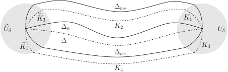
Figure 3. Contours $\Sigma$ (dashed lines) and $\Sigma_{n}^{md}$ (solid lines). Neighborhoods $U_{\delta}$ and $\widetilde{U}_{\delta}$ (disks around $\pm 1$).

It can be easily seen that the arcs $\Delta_{n\pm}$ and $\Delta$ intersect only at $\pm 1$ for all $n$ large enough since $\Delta_{n}$ approach $\Delta$ in a uniform manner by Theorem 1 and $\Delta_{n\pm}$ and $\Delta_{n}$ form angles $\pi/3$ at $1$ and $-1$ by construction.

Finally, it will be useful for us later to define one more system of contours, say $\Sigma_{n}^{md}$. The lens $\Sigma_{n}^{md}$ is obtained from $\Sigma_{n}$ simply by replacing $\Delta$ by $\Delta_{n}$ (see Fig. 3). We also require the lens $\Sigma_{ext}$ to be contained within each lens $\Sigma_{n}$ (see Fig. 2).

6.4. Extension with Controlled $\bar{\partial}$ Derivative

Without loss of generality we may assume that $\Sigma_{n}\subset D_{\Xi}$ and all the functions $h_{n}$ are holomorphic in $D_{\Xi}$. By the very definition of $c_{n}^{\pm}$ we have that

$$c_{n}^{\pm}=G_{h_{n}}\left(S_{h_{n}}^{\pm}\right)^{2}h_{n}^{-1}.$$

Thus, there is a natural holomorphic extension of each $c_{n}^{\pm}$ given by

(6.6) $$c_{n}:=G_{h_{n}}S_{h_{n}}^{2}h_{n}^{-1}\quad\mbox{in}\quad D_{\Xi}\setminus\Delta.$$

Concerning the extension of $c$, we can prove the following.

Lemma 16.

Let $\theta\in\mathrm{W}^{1-1/p}_{p}$, $p\in(2,\infty)$, or $\theta\in\mathrm{C}^{m,\varsigma}$, $m\in\mathbb{Z}_{+}$, $\varsigma\in(0,1]$, $m+\varsigma>\frac{1}{2}$. Then there exists a function $c$, continuous in $\mathbb{C}\setminus\Delta$ and up to $\Delta^{\pm}$, satisfying

$$c_{|\Delta^{\pm}}=c^{\pm},\quad c=\exp\{\mathfrak{w}\ell\}\quad\mbox{in}\quad\overline{\mathbb{C}}\setminus(\overline{\Omega_{+}\cup\Omega_{-}}),\quad\mbox{and}\quad\bar{\partial}c=cf,$$

where $\ell$ is a polynomial, $\deg(\ell)\leq 2m+1$, $f\in\mathrm{L}^{p}(\Omega_{\pm})$ when $\theta\in\mathrm{W}^{1-1/p}_{p}$, $f\in\mathrm{L}^{q}(\Omega_{\pm})$, $q\in\left(2,\frac{1}{1-\varsigma}\right)$ when $\theta\in\mathrm{C}^{0,\varsigma}$, and $f\in\mathrm{C}^{m-1,\varsigma-\epsilon}_{0}(\overline{\Omega_{\pm}})$ when $\theta\in\mathrm{C}^{m,\varsigma}$, $m\in\mathbb{N}$, and $\epsilon\in(0,\varsigma)$.

Proof.

This lemma is a straightforward consequence of (5.10), inclusion $\mathrm{C}^{0,\varsigma}\subset\mathrm{W}^{1-1/q}_{q}$ for $q\in\left(2,\frac{1}{1-\varsigma}\right)$, and Propositions 8 and 9 combined with Propositions 6 and 7. ∎

6.5. Formulation of Riemann-Hilbert-$\bar{\partial}$ Problem

In this section we reformulate RHP-$\mathscr{T}$  as a Riemann-Hilbert-$\bar{\partial}$ problem. In what follows, we understand under $c$ and $c_{n}$ the extensions obtained in Section 6.4 above. Suppose that RHP-$\mathscr{T}$  is solvable and $\mathscr{T}$ is the solution. We define a matrix function $\mathscr{S}$ on $\overline{\mathbb{C}}\setminus\Sigma_{n}$ as follows:

(6.7) $$\mathscr{S}:=\left\{\begin{array}[]{ll}\mathscr{T}\left(\begin{array}[]{cc}1&0\\ \mp r_{n}c_{n}c/w&1\end{array}\right),&\mbox{in}\ \Omega_{n\pm},\vskip 3.0pt plus 1.0pt minus 1.0pt\\ \mathscr{T},&\mbox{outside the lens}\ \Sigma_{n},\end{array}\right.$$

where the upper part, $\Omega_{n+}$, (resp. lower part, $\Omega_{n-}$) of the lens $\Sigma_{n}$ is a domain bounded by $\Delta_{n+}$ (resp. $\Delta_{n-}$) and $\Delta$. This new matrix function is no longer analytic in general in the whole domain $D$ since $c$ may not be analytic inside the extension lens $\Sigma_{ext}$. Recall, however, that by the very construction, $c$ coincides with a holomorphic function $\widetilde{c}=\exp\{\mathfrak{w}\ell\}$ outside the lens $\Sigma_{ext}$. To capture the non-analytic character of $\mathscr{S}$, we introduce the following matrix function that will represent the deviation from analyticity:

(6.8) $$\mathscr{W}_{0}:=\left\{\begin{array}[]{ll}\displaystyle\left(\begin{array}[]{cc}0&0\\ \mp r_{n}c_{n}\bar{\partial}c/w&0\end{array}\right),&\mbox{in}\ \Omega_{\pm},\vskip 3.0pt plus 1.0pt minus 1.0pt\\ \left(\begin{array}[]{cc}0&0\\ 0&0\end{array}\right),&\mbox{outside the lens}\ \Sigma_{ext}.\end{array}\right.$$

Then $\mathscr{S}$ solves the following Riemann-Hilbert-$\bar{\partial}$ problem (RH$\bar{\partial}$P-$\mathscr{S}$):

• $\mathscr{S}$ is a continuous matrix function in $\overline{\mathbb{C}}\setminus\Sigma_{n}$ and $\mathscr{S}(\infty)=\mathscr{I}$;

• $\mathscr{S}$ has continuous boundary values, $\mathscr{S}_{\pm}$, on $\Sigma_{n}^{\circ}:=\Sigma_{n}\setminus\{\pm 1\}$ and

  (6.11) $$\mathscr{S}_{+} = \mathscr{S}_{-}\left(\begin{array}[]{cc}1&0\\ r_{n}c_{n}c/w&1\end{array}\right)\quad\mbox{on}\quad\Delta_{n+}^{\circ}\cup\Delta_{n-}^{\circ},$$

  (6.14) $$\mathscr{S}_{+} = \mathscr{S}_{-}\left(\begin{array}[]{cc}0&w\\ -1/w&0\end{array}\right)\quad\mbox{on}\quad\Delta^{\circ};$$

• For $\alpha<0$, $\mathscr{S}$ has the following behavior near $z=1$:

  $$\mathscr{S}(z)=O\left(\begin{array}[]{cc}1&|1-z|^{\alpha}\\ 1&|1-z|^{\alpha}\end{array}\right),\quad\mbox{as}\quad\mathbb{C}\setminus\Sigma_{n}\ni z\to 1.$$

  For $\alpha=0$, $\mathscr{S}$ has the following behavior near $z=1$:

  $$\mathscr{S}(z)=O\left(\begin{array}[]{cc}\log|1-z|&\log|1-z|\\ \log|1-z|&\log|1-z|\end{array}\right)\mbox{as}\quad\mathbb{C}\setminus\Sigma_{n}\ni z\to 1.$$

  For $\alpha>0$, $\mathscr{S}$ has the following behavior near $z=1$:

  $$\mathscr{S}(z)=\left\{\begin{array}[]{ll}\displaystyle O\left(\begin{array}[]{cc}1&1\\ 1&1\end{array}\right),&\mbox{as}\ z\to 1\ \mbox{outside the lens}\ \Sigma_{n},\vskip 3.0pt plus 1.0pt minus 1.0pt\\ \displaystyle O\left(\begin{array}[]{cc}|1-z|^{-\alpha}&1\\ |1-z|^{-\alpha}&1\end{array}\right),&\mbox{as}\ z\to 1\ \mbox{inside the lens}\ \Sigma_{n};\end{array}\right.$$

• $\mathscr{S}$ has the same behavior when $\mathbb{C}\setminus\Sigma_{n}\ni z\to-1$ as in (c) only with $\alpha$ replaced by $\beta$ and $1-z$ replaced by $1+z$;

• $\mathscr{S}$ deviates from an analytic matrix function according to $\bar{\partial}\mathscr{S}=\mathscr{S}\mathscr{W}_{0}$.

Then the following lemma holds.

Lemma 17.

RH$\bar{\partial}$P-$\mathscr{S}$  is solvable if and only if RHP-$\mathscr{T}$  is solvable. When solutions of RH$\bar{\partial}$P-$\mathscr{S}$  and RHP-$\mathscr{T}$  exist, they are unique and connected by (6.7).

Proof.

By construction, the solution of RHP-$\mathscr{T}$  yields a solution of RH$\bar{\partial}$P-$\mathscr{S}$. Conversely, let $\mathscr{S}^{*}$ be a solution of RH$\bar{\partial}$P-$\mathscr{S}$. It is easy to check using the Leibnitz’s rule that $\bar{\partial}\mathscr{T}^{*}$ is equal to the zero matrix outside of $\Sigma_{n}$, where $\mathscr{T}^{*}$ is obtained from $\mathscr{S}^{*}$ by inverting (6.7). Thus, $\mathscr{T}^{*}$ is an analytic matrix function in $\overline{\mathbb{C}}\setminus\Sigma_{n}$ with continuous boundary values on each side of $\Sigma_{n}^{\circ}$. Moreover, it can be readily verified that $\mathscr{T}^{*}$ has no jumps on $\Delta_{n\pm}^{\circ}$ and therefore is, in fact, analytic in $D$. It is aslo obvious that it equals to the identity matrix at infinity and has a jump on $\Delta$ described by RHP-$\mathscr{T}$(b). Thus, $\mathscr{T}^{*}$ complies with RHP-$\mathscr{T}$(a)–(b).

Now, if $\alpha,\beta<0$ then it follows from RH$\bar{\partial}$P-$\mathscr{S}$(c)–(d) and (6.7) that $\mathscr{T}^{*}$ has the same behavior near endpoints $\pm 1$ as $\mathscr{S}^{*}$. Therefore, $\mathscr{T}^{*}$ solves RHP-$\mathscr{T}$  in this case. When either $\alpha$ or $\beta$ is nonnegative, it is no longer immediate that the first column of $\mathscr{T}^{*}$ has the behavior near $\pm 1$ required by RHP-$\mathscr{T}$(c)–(d). This difficulty was resolved in [33, Lem. 4.1] by considering $\mathscr{T}^{*}\mathscr{T}^{-1}$, where $\mathscr{T}$ is the unique solution of RHP-$\mathscr{T}$. However, in the present case it is not clear that such a solution exists (see Lemma 14). Thus, we are bound to consider the first column of $\mathscr{T}^{*}$ by itself.

Denote by $\mathscr{T}^{*}_{11}$ and $\mathscr{T}^{*}_{21}$ the $11$- and $21$-entries of $\mathscr{T}^{*}$. Then $\mathscr{T}^{*}_{11}$ and $\mathscr{T}^{*}_{21}$ are analytic functions in $D$ with the following behavior near $1$:

(6.15) $$\mathscr{T}^{*}_{j1}(z)=\left\{\begin{array}[]{ll}O(1),&\mbox{if}\quad\alpha<0\vskip 3.0pt plus 1.0pt minus 1.0pt\\ O(\log|1-z|),&\mbox{if}\quad\alpha=0,\vskip 3.0pt plus 1.0pt minus 1.0pt\\ O(|1-z|^{-\alpha}),&\mbox{if}\quad\alpha>0\ \mbox{and}\ z\ \mbox{is inside the lens},\vskip 3.0pt plus 1.0pt minus 1.0pt\\ O(1),&\mbox{if}\quad\alpha>0\ \mbox{and}\ z\ \mbox{is outside the lens},\end{array}\right.$$

for $j=1,2$. The behavior near $-1$ is identical only with $\alpha$ replaced by $\beta$ and $1-z$ replaced by $1+z$. Moreover, each $\mathscr{T}^{*}_{j1}$ solves the following scalar boundary value problem:

(6.16) $$\phi^{+}=\phi^{-}(r_{n}c_{n}c)^{+}\quad\mbox{on}\quad\Delta,\quad\phi\in\mathrm{H}(D).$$

Now, recall that $r_{n}^{+}r_{n}^{-}\equiv 1$ on $\Delta$ and $r_{n}$ has $2n$ zeros in $D$ that lie away from the lens $\Sigma_{n}$. Hence, the argument of $r_{n}^{+}$ increases by $2\pi n$ when $\Delta$ is traversed from $-1$ to $1$. Moreover, for $c^{+}$ and each $c_{n}^{+}$ a branch of the argument can be taken continuous and vanishing at $\pm 1$ (it is the imaginary part of $\mathfrak{w}^{+}\mathcal{S}(\theta/\mathfrak{w}^{+})$, which is continuous and vanishing at $\pm 1$ by Propositions 8 and 9). Define $\varrho:=\log(r_{n}c_{n}c)^{+}$, $\varrho(-1)=0$. This normalization is possible since $r_{n}^{+}(-1)=1$ as $r_{n}^{+}$ is a product of $2n$ factors each of which is equal to $-1$ at $-1$. Furthermore, this normalization necessarily yields that $\varrho(1)=2\pi ni$ and that the so-called canonical solution of the problem (6.16) is given by [24, Sec. 43.1]

$$\phi_{c}(z):=(z-1)^{-n}\exp\left\{\mathcal{C}(\varrho;z)\right\},\quad z\in D.$$

Recall that $\phi_{c}$ is bounded above and below in the vicinities of 1 and $-1$, has a zero of order $n$ at infinity, and otherwise is non-vanishing. Hence, the functions $\phi_{j}:=\mathscr{T}^{*}_{j1}/\phi_{c}$, $j=1,2$, are analytic in $\mathbb{C}\setminus\{\pm 1\}$. Moreover, according to (6.15), the singularities of these functions at 1 and $-1$ cannot be essential, they are either removable or polar. In fact, since $\phi_{j}(z)=O(1)$ or $\phi_{j}(z)=O(\log|1\pm z|)$ when $z$ approaches 1 or $-1$ outside of the lens, $\phi_{j}$ can have only removable singularities at these points. Hence, $\phi_{j}(z)=O(1)$ and subsequently $\mathscr{T}^{*}_{j1}=O(1)$ near 1 and $-1$. Thus, $\mathscr{T}^{*}$ satisfies RHP-$\mathscr{T}$(c)–(d) for all $\alpha$ and $\beta$, which means that $\mathscr{T}^{*}$ is the solution of RHP-$\mathscr{T}$. Therefore, indeed, the problems RHP-$\mathscr{T}$  and RH$\bar{\partial}$P-$\mathscr{S}$  are equivalent. ∎

7. Analytic Approximation of RH$\bar{\partial}$P-$\mathscr{S}$

Elaborating on the path developed in [37], we put RH$\bar{\partial}$P-$\mathscr{S}$  aside for a while and consider an analytic approximation of this problem. In other words, we seek the solution of the following Riemann-Hilbert problem (RHP-$\mathscr{A}$):

• $\mathscr{A}$ is a holomorphic matrix function in $\overline{\mathbb{C}}\setminus\Sigma_{n}$ and $\mathscr{A}(\infty)=\mathscr{I}$;

• $\mathscr{A}$ has continuous traces, $\mathscr{A}_{\pm}$, on $\Sigma_{n}^{\circ}$ that satisfy the same relations as in RH$\bar{\partial}$P-$\mathscr{S}$(b);

• the behavior of $\mathscr{A}$ near 1 is described by RH$\bar{\partial}$P-$\mathscr{S}$(c);

• the behavior of $\mathscr{A}$ near $-1$ is described by RH$\bar{\partial}$P-$\mathscr{S}$(d).

Before we proceed, observe that the function $c$ coincides on $\Delta_{n\pm}$ with the analytic function $\widetilde{c}:=\exp\{\mathfrak{w}\ell\}$, where $\ell$ is a polynomial, by construction. Hence, we can assume that the jump matrix in RHP-$\mathscr{A}$(b) is expressed in terms of $\widetilde{c}$ rather than $c$.

7.1. Modified RHP-$\mathscr{A}$

The problem above almost falls into the scope of the classical approach to asymptotics of orthogonal polynomials. We say “almost” because it is not generally true that the functions $r_{n}$ can be written as the $2n$-th power of a single function, even up to a normal family as is the case in [3, Thm. 2]. This will explain why we constructed another lens, $\Sigma_{n}^{md}$, in Section 6.3.

Consider the following Riemann-Hilbert problem (RHP-$\mathscr{B}$):

• $\mathscr{B}$ is a holomorphic matrix function in $\overline{\mathbb{C}}\setminus\Sigma_{n}^{md}$ and $\mathscr{B}(\infty)=\mathscr{I}$;

• $\mathscr{B}$ has continuous traces, $\mathscr{B}_{\pm}$, on $(\Sigma_{n}^{md})^{\circ}$ that satisfy

  $$\begin{array}[]{llll}\mathscr{B}_{+}&=&\mathscr{B}_{-}\left(\begin{array}[]{cc}1&0\\ r_{n}c_{n}\widetilde{c}/w&1\end{array}\right)&\mbox{on}\quad\Delta_{n+}^{\circ}\cup\Delta_{n-}^{\circ},\vskip 3.0pt plus 1.0pt minus 1.0pt\\ \mathscr{B}_{+}&=&\mathscr{B}_{-}\left(\begin{array}[]{cc}0&w\\ -1/w&0\end{array}\right)&\mbox{on}\quad\Delta_{n}^{\circ};\end{array}$$

• the behavior of $\mathscr{B}$ near 1 is described by RHP-$\mathscr{A}$(c) with respect to the lens $\Sigma_{n}^{md}$;

• the behavior of $\mathscr{B}$ near $-1$ is described by RHP-$\mathscr{A}$(d), again, with respect to $\Sigma_{n}^{md}$.

In fact, this new problem is equivalent to RHP-$\mathscr{A}$.

Lemma 18.

The problems RHP-$\mathscr{A}$  and RHP-$\mathscr{B}$  are equivalent.

Proof.

Suppose that RHP-$\mathscr{B}$  is solvable and $\mathscr{B}$ is a solution. As before, let $\Omega_{n+}$ (resp. $\Omega_{n-}$) be the upper (resp. lower) part of the lens $\Sigma_{n}$. Analogously define $\Omega_{n\pm}^{md}$ and set

(7.1) $$\mathscr{A}^{*}:=\left\{\begin{array}[]{ll}\mathscr{B}\left(\begin{array}[]{cc}0&w\\ -1/w&0\end{array}\right),&\mbox{in}\quad\Omega_{n+}\cap\Omega_{n-}^{md},\vskip 3.0pt plus 1.0pt minus 1.0pt\\ \mathscr{B}\left(\begin{array}[]{cc}0&-w\\ 1/w&0\end{array}\right),&\mbox{in}\quad\Omega_{n-}\cap\Omega_{n+}^{md},\vskip 3.0pt plus 1.0pt minus 1.0pt\\ \mathscr{B},&\mbox{elsewhere}.\end{array}\right.$$

Observe that $\Omega_{n\pm}\cap\Omega^{md}_{n\mp}$ is a finite, possibly empty, union of Jordan domains by analyticity of $\Delta$ and $\Delta_{n}$. It is a routine exercise to verify that $\mathscr{A}^{*}$ complies with RHP-$\mathscr{A}$(a) and (b). Moreover, within $\Omega_{n+}\cap\Omega_{n-}^{md}$ and $\Omega_{n-}\cap\Omega_{n+}^{md}$ we have that for $\alpha<0$, $\mathscr{A}^{*}$ has the following behavior near $z=1$:

$$\mathscr{A}^{*}(z)=O\left(\begin{array}[]{cc}1&|1-z|^{\alpha}\\ 1&|1-z|^{\alpha}\end{array}\right)O\left(\begin{array}[]{cc}0&|1-z|^{\alpha}\\ |1-z|^{-\alpha}&0\end{array}\right)=O\left(\begin{array}[]{cc}1&|1-z|^{\alpha}\\ 1&|1-z|^{\alpha}\end{array}\right),$$

as $z\to 1$; for $\alpha=0$, $\mathscr{A}^{*}$ has the same behavior near $z=1$ as $\mathscr{B}$ since the latter is multiplied by a bounded matrix near $1$; for $\alpha>0$, $\mathscr{A}^{*}$ has the following behavior near $z=1$:

$$\mathscr{A}^{*}(z)=O\left(\begin{array}[]{cc}|1-z|^{-\alpha}&1\\ |1-z|^{-\alpha}&1\end{array}\right)O\left(\begin{array}[]{cc}0&|1-z|^{\alpha}\\ |1-z|^{-\alpha}&0\end{array}\right)=O\left(\begin{array}[]{cc}|1-z|^{-\alpha}&1\\ |1-z|^{-\alpha}&1\end{array}\right).$$

Hence, $\mathscr{A}^{*}$ has exactly the behavior near $1$ required by RHP-$\mathscr{A}$(c). In the same fashion one can check that $\mathscr{A}^{*}$ satisfies RHP-$\mathscr{A}$(d)  and therefore it is, in fact, a solution of RHP-$\mathscr{A}$. Clearly, the arguments above could be reversed and hence each solution of RHP-$\mathscr{A}$  yields a solution of RHP-$\mathscr{B}$. ∎

Let us now alleviate the notation by making a slightly abuse of it. Throughout this section, we shall understand under $\varphi$, $r_{n}$, $g_{n}$, $\widetilde{g}_{n}$, $c_{n}$, $\widetilde{c}$, $\mathfrak{w}$, $S_{h_{n}}$, $S_{\mathfrak{w}^{+}}$, and $S_{w}$ their holomorphic continuations that are analytic outside of $\Delta_{n}$ rather than $\Delta$. Note that outside the bounded set with boundary $\Delta\cup\Delta_{n}$ these continued functions coincide with the original ones. Moreover, their values considered within the interior domain of $\Delta_{n}\cup\Delta$ can be obtained through analytic continuation of the original functions across $\Delta$.

7.2. Auxiliary Riemann-Hilbert Problems

In this subsection we define the necessary objects to solve RHP-$\mathscr{B}$. This material essentially appeared in [33] for the case $\Delta=[-1,1]$.

7.2.1. Parametrix away from the endpoints

As $r_{n}$ converges to zero geometrically fast away from $\Delta_{n}$, the jump matrix in RHP-$\mathscr{B}$(b)  is close to the identity on $\Delta_{n+}^{\circ}$ and $\Delta_{n-}^{\circ}$. Thus, the main term of the asymptotics for $\mathscr{B}$ in $D_{n}=\overline{\mathbb{C}}\setminus\Delta_{n}$ is determined by the following Riemann-Hilbert problem (RHP-$\mathscr{N}$):

• $\mathscr{N}$ is a holomorphic matrix function in $D_{n}$ and $\mathscr{N}(\infty)=\mathscr{I}$;

• $\mathscr{N}$ has continuous traces, $\mathscr{N}_{\pm}$, on $\Delta_{n}^{\circ}$ and $\mathscr{N}_{+}=\mathscr{N}_{-}\left(\begin{array}[]{cc}0&w\\ -1/w&0\end{array}\right)$;

It can be easily checked using (5.14) that a solution of RHP-$\mathscr{N}$  when $w\equiv 1$ is given by

(7.2) $$\mathscr{N_{*}}=\left(\begin{array}[]{cc}\displaystyle S_{\mathfrak{w}^{+}}^{-1}&\displaystyle i(\varphi S_{\mathfrak{w}^{+}})^{-1}\vskip 3.0pt plus 1.0pt minus 1.0pt\\ \displaystyle-i(\varphi S_{\mathfrak{w}^{+}})^{-1}&S_{\mathfrak{w}^{+}}^{-1}\end{array}\right).$$

Then a solution of RHP-$\mathscr{N}$  for arbitrary $w$ is given by

(7.3) $$\mathscr{N}=(G_{w})^{\sigma_{3}/2}\mathscr{N}_{*}(G_{w}S_{w}^{2})^{-\sigma_{3}/2}.$$

7.2.2. Auxiliary parametrix near the endpoints

The following construction was introduced in [33, Thm. 6.3]. Let $I_{\alpha}$ and $K_{\alpha}$ be the modified Bessel functions and $H_{\alpha}^{(1)}$ and $H_{\alpha}^{(2)}$ be the Hankel functions [1, Ch. 9]. Set $\Psi$ to be the following sectionally holomorphic matrix function:

$$\Psi(\zeta)=\Psi(\zeta;\alpha):=\left(\begin{array}[]{cc}I_{\alpha}\left(2\zeta^{1/2}\right)&\frac{i}{\pi}K_{\alpha}\left(2\zeta^{1/2}\right)\vskip 3.0pt plus 1.0pt minus 1.0pt\\ 2\pi i\zeta^{1/2}I_{\alpha}^{\prime}\left(2\zeta^{1/2}\right)&-2\zeta^{1/2}K_{\alpha}^{\prime}\left(2\zeta^{1/2}\right)\end{array}\right)$$

for $|\textnormal{Arg}(\zeta)|<2\pi/3$;

$$\Psi(\zeta):=\left(\begin{array}[]{cc}\frac{1}{2}H_{\alpha}^{(1)}\left(2(-\zeta)^{1/2}\right)&\frac{1}{2}H_{\alpha}^{(2)}\left(2(-\zeta)^{1/2}\right)\vskip 3.0pt plus 1.0pt minus 1.0pt\\ \pi\zeta^{1/2}\left(H_{\alpha}^{(1)}\right)^{\prime}\left(2(-\zeta)^{1/2}\right)&\pi\zeta^{1/2}\left(H_{\alpha}^{(2)}\right)^{\prime}\left(2(-\zeta)^{1/2}\right)\end{array}\right)e^{\frac{1}{2}\alpha\pi i\sigma_{3}}$$

for $2\pi/3<\textnormal{Arg}(\zeta)<\pi$;

$$\Psi(\zeta):=\left(\begin{array}[]{cc}\frac{1}{2}H_{\alpha}^{(2)}\left(2(-\zeta)^{1/2}\right)&-\frac{1}{2}H_{\alpha}^{(1)}\left(2(-\zeta)^{1/2}\right)\vskip 3.0pt plus 1.0pt minus 1.0pt\\ -\pi\zeta^{1/2}\left(H_{\alpha}^{(2)}\right)^{\prime}\left(2(-\zeta)^{1/2}\right)&\pi\zeta^{1/2}\left(H_{\alpha}^{(1)}\right)^{\prime}\left(2(-\zeta)^{1/2}\right)\end{array}\right)e^{-\frac{1}{2}\alpha\pi i\sigma_{3}}$$

for $-\pi<\textnormal{Arg}(\zeta)<-2\pi/3$, where $\textnormal{Arg}(\zeta)\in(-\pi,\pi]$ is the principal determination of the argument of $\zeta$. Let further $\Sigma_{1}$, $\Sigma_{2}$, and $\Sigma_{3}$ be the rays $\{\zeta:\textnormal{Arg}(\zeta)=2\pi/3\}$, $\{\zeta:\textnormal{Arg}(\zeta)=\pi\}$, and $\{\zeta:\textnormal{Arg}(\zeta)=-2\pi/3\}$, respectively, oriented from infinity to zero. Using known properties of $I_{\alpha}$, $K_{\alpha}$, $H_{\alpha}^{(1)}$, $H_{\alpha}^{(2)}$, and their derivatives, it can be checked that $\Psi$ is the solution of the following Riemann-Hilbert problem RHP-$\Psi$:

• $\Psi$ is a holomorphic matrix function in $\mathbb{C}\setminus(\Sigma_{1}\cup\Sigma_{2}\cup\Sigma_{3})$;

• $\Psi$ has continuous traces, $\Psi_{\pm}$, on $\Sigma^{\circ}_{j}$, $j\in\{1,2,3\}$, and

  $$\begin{array}[]{llll}\Psi_{+}&=&\Psi_{-}\left(\begin{array}[]{cc}1&0\\ e^{\alpha\pi i}&1\end{array}\right)&\mbox{on}\quad\Sigma_{1}^{\circ},\vskip 3.0pt plus 1.0pt minus 1.0pt\\ \Psi_{+}&=&\Psi_{-}\left(\begin{array}[]{cc}0&1\\ -1&0\end{array}\right)&\mbox{on}\quad\Sigma_{2}^{\circ},\vskip 3.0pt plus 1.0pt minus 1.0pt\\ \Psi_{+}&=&\Psi_{-}\left(\begin{array}[]{cc}1&0\\ e^{-\alpha\pi i}&1\end{array}\right)&\mbox{on}\quad\Sigma_{3}^{\circ};\end{array}$$

• $\Psi$ has the following behavior near $\infty$:

  $$\Psi(\zeta)=\left(2\pi\zeta^{1/2}\right)^{-\sigma_{3}/2}\frac{1}{\sqrt{2}}\left(\begin{array}[]{cc}1+O\left(\zeta^{-1/2}\right)&i+O\left(\zeta^{-1/2}\right)\vskip 3.0pt plus 1.0pt minus 1.0pt\\ i+O\left(\zeta^{-1/2}\right)&1+O\left(\zeta^{-1/2}\right)\end{array}\right)e^{2\zeta^{1/2}\sigma_{3}}$$

  uniformly in $\mathbb{C}\setminus(\Sigma_{1}\cup\Sigma_{2}\cup\Sigma_{3})$;

• For $\alpha<0$, $\Psi$ has the following behavior near $0$:

  $$\Psi=O\left(\begin{array}[]{cc}|\zeta|^{\alpha/2}&|\zeta|^{\alpha/2}\\ |\zeta|^{\alpha/2}&|\zeta|^{\alpha/2}\end{array}\right)\ \mbox{as}\ \zeta\to 0;$$

  For $\alpha=0$, $\Psi$ has the following behavior near $0$:

  $$\Psi=O\left(\begin{array}[]{cc}\log|\zeta|&\log|\zeta|\\ \log|\zeta|&\log|\zeta|\end{array}\right)\ \mbox{as}\ \zeta\to 0;$$

  For $\alpha>0$, $\Psi$ has the following behavior near $0$:

  $$\Psi=\left\{\begin{array}[]{ll}\displaystyle O\left(\begin{array}[]{cc}|\zeta|^{\alpha/2}&|\zeta|^{-\alpha/2}\\ |\zeta|^{\alpha/2}&|\zeta|^{-\alpha/2}\end{array}\right)&\mbox{as}\ \zeta\to 0\ \mbox{in}\ |\textnormal{Arg}(\zeta)|<2\pi/3,\vskip 3.0pt plus 1.0pt minus 1.0pt\\ \displaystyle O\left(\begin{array}[]{cc}|\zeta|^{-\alpha/2}&|\zeta|^{-\alpha/2}\\ |\zeta|^{-\alpha/2}&|\zeta|^{-\alpha/2}\end{array}\right)&\mbox{as}\ \zeta\to 0\ \mbox{in}\ 2\pi/3<|\textnormal{Arg}(\zeta)|<\pi.\end{array}\right.$$

Further, if we set

$$\widetilde{\Psi}:=\sigma_{3}\Psi(\cdot;\beta)\sigma_{3},$$

then this matrix function satisfies RHP-$\Psi$  with $\alpha$ replaced by $\beta$ and reversed orientation for $\Sigma_{j}$, $j\in\{1,2,3\}$.

7.2.3. Parametrix near $1$

As shown in [33], the main term of the asymptotics of the solution of RHP-$\mathscr{B}$  near the endpoints of $\Delta_{n}$ is described by a solution of a special Riemann-Hilbert problem for which $\Psi$ will be instrumental. Let $U_{\delta}$ be as in the construction of $\Sigma_{n}$ (see Section 6.3). Below we describe the solution of the following Riemann-Hilbert problem (RHP-$\mathscr{P}$):

• $\mathscr{P}$ is a holomorphic matrix function in $U_{\delta}\setminus\Sigma_{n}^{md}$;

• $\mathscr{P}$ has continuous boundary values, $\mathscr{P}_{\pm}$, on $U_{\delta}\cap(\Sigma_{n}^{md})^{\circ}$ and

  $$\begin{array}[]{llll}\mathscr{P}_{+}&=&\mathscr{P}_{-}\left(\begin{array}[]{cc}1&0\\ r_{n}c_{n}\widetilde{c}/w&1\end{array}\right)&\mbox{on}\quad U_{\delta}\cap(\Delta_{n+}^{\circ}\cup\Delta_{n-}^{\circ}),\vskip 3.0pt plus 1.0pt minus 1.0pt\\ \mathscr{P}_{+}&=&\mathscr{P}_{-}\left(\begin{array}[]{cc}0&w\\ -1/w&0\end{array}\right)&\mbox{on}\quad U_{\delta}\cap\Delta_{n}^{\circ};\end{array}$$

• $\mathscr{P}\mathscr{N}^{-1}=\mathscr{I}+O(1/n)$ uniformly on $\partial U_{\delta}$;

• For $\alpha<0$, $\mathscr{P}$ has the following behavior near $z=1$:

  $$\mathscr{P}=O\left(\begin{array}[]{cc}1&|1-z|^{\alpha}\\ 1&|1-z|^{\alpha}\end{array}\right),\quad\mbox{as}\quad U_{\delta}\setminus\Sigma_{n}^{md}\ni z\to 1;$$

  For $\alpha=0$, $\mathscr{P}$ has the following behavior near $z=1$:

  $$\mathscr{P}=O\left(\begin{array}[]{cc}\log|1-z|&\log|1-z|\\ \log|1-z|&\log|1-z|\end{array}\right),\quad\mbox{as}\quad U_{\delta}\setminus\Sigma_{n}^{md}\ni z\to 1;$$

  For $\alpha>0$, $\mathscr{P}$ has the following behavior near $z=1$:

  $$\mathscr{P}=\left\{\begin{array}[]{ll}\displaystyle O\left(\begin{array}[]{cc}1&1\\ 1&1\end{array}\right),&\mbox{as}\ z\to 1\ \mbox{outside the lens}\ \Sigma_{n}^{md},\vskip 3.0pt plus 1.0pt minus 1.0pt\\ \displaystyle O\left(\begin{array}[]{cc}|1-z|^{-\alpha}&1\\ |1-z|^{-\alpha}&1\end{array}\right),&\mbox{as}\ z\to 1\ \mbox{inside the lens}\ \Sigma_{n}^{md}.\end{array}\right.$$

To present a solution of RHP-$\mathscr{P}$, we need to introduce more notation. Denote by $U_{\delta}^{+}$ and $U_{\delta}^{-}$ the subsets of $U_{\delta}$ that are mapped by $g_{n}^{2}$ into the upper and lower half planes, respectively. Without loss of generality we may assume that functions $\theta_{n}$ are holomorphic in $U_{\delta}$ and the branch cut of $w$ in $U_{\delta}$ coincides with the preimage of the positive reals under $g^{2}_{n}$. In particular, we have that $w$ is analytic in $U^{+}_{\delta}$ and $U_{\delta}^{-}$ and therefore across $\Delta_{n\pm}^{\circ}$. Set

$$A_{n}(z):=\frac{\exp\left\{\frac{1}{2}\left(\theta_{n}(z)-\mathfrak{w}(z)\ell(z)\right)\right\}}{\sqrt{G_{h_{n}}}S_{h_{n}}(z)}(z-1)^{\alpha/2}(z+1)^{\beta/2},$$

where we use the same branch of $(z+1)^{\beta/2}$ as in definition of $w$ and a branch of $(z-1)^{\alpha/2}$ analytic in $U_{\delta}\setminus\Delta_{n}$ and positive for positive reals large enough. Then

(7.4) $$A_{n}^{2}=\left\{\begin{array}[]{ll}e^{\alpha\pi i}w/c_{n}\widetilde{c},&\mbox{in}\quad U_{\delta}^{+},\vskip 3.0pt plus 1.0pt minus 1.0pt\\ e^{-\alpha\pi i}w/c_{n}\widetilde{c},&\mbox{in}\quad U_{\delta}^{-},\end{array}\right.$$

by the definition of $\widetilde{c}$ and on account of (6.6). Moreover, it readily follows from (7.4) and (6.3) that

(7.5) $$A^{+}_{n}A^{-}_{n}=w\quad\mbox{on}\quad\Delta_{n}^{\circ}.$$

Observe that $g_{n}^{1/2}$ is a holomorphic function on $U_{\delta}\setminus\Delta_{n}$ such that

(7.6) $$(g_{n}^{1/2})^{+}=i(g_{n}^{1/2})^{-}\quad\mbox{on}\quad\Delta_{n}$$

by (3.8). Then the following lemma holds.

Lemma 19.

A solution of RHP-$\mathscr{P}$  is given by

$$\mathscr{P}=\mathscr{E}\Psi\left(\frac{n^{2}g_{n}^{2}}{4}\right)A_{n}^{-\sigma_{3}}r_{n}^{\sigma_{3}/2},\quad\mathscr{E}:=\mathscr{N}A_{n}^{\sigma_{3}}\frac{1}{\sqrt{2}}\left(\begin{array}[]{cc}1&-i\\ -i&1\end{array}\right)\left(\pi ng_{n}\right)^{\sigma_{3}/2}.$$

Proof.

Except for some technical differences, the proof is analogous to the considerations in [33, eqn. (6.27) and after]. First, we must show that $\mathscr{E}$ is holomorphic in $U_{\delta}$. This is clearly true in $U_{\delta}\setminus\Delta_{n}$. It is also clear that $\mathscr{E}$ has continuous boundary values on each side of $\Delta_{n}^{\circ}$. Since

(7.9) $$\mathscr{E}_{+} = \mathscr{N}_{+}\left(A_{n}^{+}\right)^{\sigma_{3}}\frac{1}{\sqrt{2}}\left(\begin{array}[]{cc}1&-i\\ -i&1\end{array}\right)(\pi n)^{\sigma_{3}/2}\left(\left(g_{n}^{1/2}\right)^{+}\right)^{\sigma_{3}}$$

(7.16) $$= \mathscr{N}_{-}\left(\begin{array}[]{cc}0&w\\ -1/w&0\end{array}\right)\left(\frac{w}{A_{n}^{-}}\right)^{\sigma_{3}}\frac{1}{\sqrt{2}}\left(\begin{array}[]{cc}1&-i\\ -i&1\end{array}\right)(\pi n)^{\sigma_{3}/2}\left(\begin{array}[]{cc}i&0\\ 0&-i\end{array}\right)\left(\left(g_{n}^{1/2}\right)^{-}\right)^{\sigma_{3}}$$

(7.21) $$= \mathscr{N}_{-}\left(A_{n}^{-}\right)^{\sigma_{3}}\left(\begin{array}[]{cc}0&1\\ -1&0\end{array}\right)\frac{1}{\sqrt{2}}\left(\begin{array}[]{cc}i&-1\\ 1&-i\end{array}\right)(\pi n)^{\sigma_{3}/2}\left(\left(g_{n}^{1/2}\right)^{-}\right)^{\sigma_{3}}=\mathscr{E}_{-},$$

where we used RHP-$\mathscr{N}$(b), (7.5), and (7.6), $\mathscr{E}$ is holomorphic across $\Delta_{n}^{\circ}$. Thus, it remains to show that $\mathscr{E}$ has no singularity at 1. For this observe that

$$\left(g_{n}^{1/2}(z)\right)^{\sigma_{3}}=O\left(\begin{array}[]{cc}|1-z|^{1/4}&0\\ 0&|1-z|^{-1/4}\end{array}\right),\quad\mbox{as}\quad z\to 1,$$

since $g_{n}^{2}$ has a simple zero at 1. Furthermore, by the very definition it holds that

$$\mathscr{N}_{*}=O\left(\begin{array}[]{cc}|1-z|^{-1/4}&|1-z|^{-1/4}\\ |1-z|^{-1/4}&|1-z|^{-1/4}\end{array}\right),\quad\mbox{as}\quad z\to 1.$$

Finally, $\displaystyle(A_{n}/S_{w})(z)\to 2^{-(\alpha+\beta)/2}$ as $z\to 1$ by (5.12). Hence, the entries of $\mathscr{E}$ can have at most square-root singularity at 1, which is impossible since $\mathscr{E}$ is analytic in $U_{\delta}\setminus\{1\}$, and therefore $\mathscr{E}$ is analytic in the whole disk $U_{\delta}$.

The analyticity of $\mathscr{E}$ implies that the jumps of $\mathscr{P}$ are those of $\Psi\left(n^{2}g_{n}^{2}/4\right)A_{n}^{-\sigma_{3}}r_{n}^{\sigma_{3}/2}$. Clearly, the latter has jumps on $\Sigma_{n}^{md}\cap U_{\delta}$ by the very definition of $g_{n}^{2}$ and $\Psi$. Moreover, it is a routine exercise, using RHP-$\Psi$(b) and (7.4), to verify that these jumps are described exactly by RHP-$\mathscr{P}$(b). It is also clear that RHP-$\mathscr{P}$(a) is satisfied. Further, we get directly from RHP-$\Psi$(c) that the behavior of $\Psi\left(n^{2}g_{n}^{2}/4\right)$ on $\partial U_{\delta}$ can be described by

$$\Psi\left(\frac{n^{2}g_{n}^{2}}{4}\right)=(\pi ng_{n})^{-\sigma_{3}/2}\left(\begin{array}[]{cc}\displaystyle 1+O\left(1/n\right)&\displaystyle i+O\left(1/n\right)\vskip 3.0pt plus 1.0pt minus 1.0pt\\ \displaystyle i+O\left(1/n\right)&\displaystyle 1+O\left(1/n\right)\end{array}\right)r_{n}^{-\sigma_{3}/2},$$

where the property $O(1/n)$ holds uniformly on $\partial U_{\delta}$. Hence, using that the diagonal matrices $A_{n}^{-\sigma_{3}}$ and $r_{n}^{\sigma_{3}/2}$ commute, we get that

$$\mathscr{P}\mathscr{N}^{-1} = \mathscr{E}\left(\pi ng_{n}\right)^{-\sigma_{3}/2}\left(\begin{array}[]{cc}\displaystyle 1+O\left(1/n\right)&\displaystyle i+O\left(1/n\right)\vskip 3.0pt plus 1.0pt minus 1.0pt\\ \displaystyle i+O\left(1/n\right)&\displaystyle 1+O\left(1/n\right)\end{array}\right)A_{n}^{-\sigma_{3}}\mathscr{N}^{-1}$$

$$= \mathscr{N}A_{n}^{\sigma_{3}}\left(\mathscr{I}+O\left(1/n\right)\right)A_{n}^{-\sigma_{3}}\mathscr{N}^{-1}=\mathscr{I}+O\left(1/n\right)$$

since the moduli of all the entries of $\mathscr{N}A_{n}^{\sigma_{3}}$ are uniformly bounded above and away from zero on $\partial U_{\delta}$. Thus, RHP-$\mathscr{P}$(c)  holds. Finally, RHP-$\mathscr{P}$(d)  follows immediately from RHP-$\Psi$(d)  upon recalling that $|g_{n}^{2}(z)|=O(|1-z|)$ and $|A_{n}(z)|\sim|1-z|^{\alpha/2}$ as $z\to 1$. ∎

7.2.4. Parametrix near $-1$

In this section we describe the solution of the Riemann-Hilbert problem that plays the same role with respect to $-1$ as RHP-$\mathscr{P}$  did for 1. Below we describe the solution of the following Riemann-Hilbert problem (RHP-$\mathscr{\widetilde{P}}$):

• $\mathscr{\widetilde{P}}$ is a holomorphic matrix function in $\widetilde{U}_{\delta}\setminus\Sigma_{n}^{md}$;

• $\mathscr{\widetilde{P}}$ has continuous boundary values, $\mathscr{\widetilde{P}}_{\pm}$, on $\widetilde{U}_{\delta}\cap(\Sigma_{n}^{md})^{\circ}$ and

  $$\begin{array}[]{llll}\mathscr{\widetilde{P}}_{+}&=&\mathscr{\widetilde{P}}_{-}\left(\begin{array}[]{cc}1&0\\ r_{n}c_{n}\widetilde{c}/w&1\end{array}\right)&\mbox{on}\quad\widetilde{U}_{\delta}\cap(\Delta_{n+}^{\circ}\cup\Delta_{n-}^{\circ}),\vskip 3.0pt plus 1.0pt minus 1.0pt\\ \mathscr{\widetilde{P}}_{+}&=&\mathscr{\widetilde{P}}_{-}\left(\begin{array}[]{cc}0&w\\ -1/w&0\end{array}\right)&\mbox{on}\quad\widetilde{U}_{\delta}\cap\Delta_{n}^{\circ};\end{array}$$

• $\mathscr{\widetilde{P}}\mathscr{N}^{-1}=\mathscr{I}+O(1/n)$ uniformly on $\partial\widetilde{U}_{\delta}$;

• For $\beta<0$, $\mathscr{\widetilde{P}}$ has the following behavior near $z=-1$:

  $$\mathscr{\widetilde{P}}=O\left(\begin{array}[]{cc}1&|1+z|^{\beta}\\ 1&|1+z|^{\beta}\end{array}\right),\quad\mbox{as}\quad\widetilde{U}_{\delta}\setminus\Sigma_{n}^{md}\ni z\to-1;$$

  For $\beta=0$, $\mathscr{\widetilde{P}}$ has the following behavior near $z=-1$:

  $$\mathscr{\widetilde{P}}=O\left(\begin{array}[]{cc}\log|1+z|&\log|1+z|\\ \log|1+z|&\log|1+z|\end{array}\right),\quad\mbox{as}\quad\widetilde{U}_{\delta}\setminus\Sigma_{n}^{md}\ni z\to-1;$$

  For $\beta>0$, $\mathscr{\widetilde{P}}$ has the following behavior near $z=-1$:

  $$\mathscr{\widetilde{P}}=\left\{\begin{array}[]{ll}\displaystyle O\left(\begin{array}[]{cc}1&1\\ 1&1\end{array}\right),&\mbox{as}\ z\to-1\ \mbox{outside the lens}\ \Sigma_{n}^{md},\vskip 3.0pt plus 1.0pt minus 1.0pt\\ \displaystyle O\left(\begin{array}[]{cc}|1+z|^{-\beta}&1\\ |1+z|^{-\beta}&1\end{array}\right),&\mbox{as}\ z\to-1\ \mbox{inside the lens}\ \Sigma_{n}^{md}.\end{array}\right.$$

This problem is solved exactly in the same manner as RHP-$\mathscr{P}$. Thus, we set

$$\widetilde{A}_{n}(z):=\frac{\exp\left\{\frac{1}{2}\left(\theta_{n}(z)-\mathfrak{w}(z)\ell(z)\right)\right\}}{\sqrt{G_{h_{n}}}S_{h_{n}}(z)}(1-z)^{\alpha/2}(-1-z)^{\beta/2},$$

where the branch of $(1-z)^{\alpha/2}$ is the same as the corresponding one in $w$, and $(-1-z)^{\beta/2}$ is holomorphic in $\widetilde{U}_{\delta}\setminus\Delta_{n}$ and positive for negative real large enough. As in (7.4), we have that

$$\widetilde{A}_{n}^{2}=\left\{\begin{array}[]{ll}e^{\beta\pi i}w/c_{n}\widetilde{c},&\mbox{in}\quad\widetilde{U}_{\delta}^{+},\vskip 3.0pt plus 1.0pt minus 1.0pt\\ e^{-\beta\pi i}w/c_{n}\widetilde{c},&\mbox{in}\quad\widetilde{U}_{\delta}^{-},\end{array}\right.$$

where $\widetilde{U}_{\delta}^{\pm}$ have the same meaning as in the previous section. However, here one needs to be cautious since $\widetilde{g}_{n}$ reverses the orientation on $\Sigma_{2}$, i.e. $\Sigma_{2}$ is now oriented from zero to infinity, and therefore $\widetilde{U}_{\delta}^{+}$ is mapped into $\{z:~{}\textnormal{Im}(z)<0\}$ and $\widetilde{U}_{\delta}^{-}$ into $\{z:~{}\textnormal{Im}(z)>0\}$. Again, it can be checked that

$$\widetilde{A}^{+}_{n}\widetilde{A}^{-}_{n}=w\quad\mbox{on}\quad\Delta_{n}^{\circ}.$$

The following lemma can be proven exactly as Lemma 19 using that $(-1)^{n}r_{n}^{1/2}=e^{n\widetilde{g}_{n}}$.

Lemma 20.

The solution of RHP-$\mathscr{\widetilde{P}}$  is given by

$$\mathscr{\widetilde{P}}=\mathscr{\widetilde{E}}\widetilde{\Psi}\left(\frac{n^{2}\widetilde{g}_{n}^{2}}{4}\right)\widetilde{A}_{n}^{-\sigma_{3}}(-1)^{n\sigma_{3}}r_{n}^{\sigma_{3}/2},\ \mathscr{\widetilde{E}}:=\mathscr{N}\widetilde{A}_{n}^{\sigma_{3}}\frac{1}{\sqrt{2}}\left(\begin{array}[]{cc}1&i\\ i&1\end{array}\right)\left(\pi n\widetilde{g}_{n}\right)^{\sigma_{3}/2}.$$

Finally, we are prepared to solve RHP-$\mathscr{A}$.

7.3. Solution of RHP-$\mathscr{A}$

Denote by $\Sigma^{rd}_{n}$ the reduced system of contours obtained from $\Sigma_{n}^{md}$ by removing $\Delta_{n}$ and $\Delta_{n\pm}\cap(U_{\delta}\cup\widetilde{U}_{\delta})$ and adding $\partial U_{\delta}\cup\partial\widetilde{U}_{\delta}$. For this new system of contours we consider the following Riemann-Hilbert problem (RHP-$\mathscr{R}$):

• $\mathscr{R}$ is a holomorphic matrix function in $\overline{\mathbb{C}}\setminus\Sigma_{n}^{rd}$ and $\mathscr{R}(\infty)=\mathscr{I}$;

• the traces of $\mathscr{R}$, $\mathscr{R}_{\pm}$, are continuous on $\Sigma^{rd}_{n}$ except for the branching points of $\Sigma^{rd}_{n}$, where they have definite limits from each sector and along each branch of $\Sigma_{n}^{rd}$. Moreover, $\mathscr{R}_{\pm}$ satisfy

  $$\mathscr{R}_{+}=\mathscr{R}_{-}\left\{\begin{array}[]{ll}\mathscr{P}\mathscr{N}^{-1}&\mbox{on}\quad\partial U_{\delta},\vskip 3.0pt plus 1.0pt minus 1.0pt\\ \mathscr{\widetilde{P}}\mathscr{N}^{-1}&\mbox{on}\quad\partial\widetilde{U}_{\delta}\vskip 3.0pt plus 1.0pt minus 1.0pt\\ \mathscr{N}\left(\begin{array}[]{cc}1&0\\ r_{n}c_{n}\widetilde{c}/w&1\end{array}\right)\mathscr{N}^{-1}&\mbox{on}\quad\Sigma_{n}^{rd}\setminus(\partial U_{\delta}\cup\partial\widetilde{U}_{\delta}).\end{array}\right.$$

Then the following lemma takes place.

Lemma 21.

The solution of RHP-$\mathscr{R}$  exists for all $n$ large enough and satisfies

(7.25) $$\mathscr{R}=\mathscr{I}+O\left(1/n\right),$$

where $O(1/n)$ holds uniformly in $\overline{\mathbb{C}}$. Moreover, $\det(\mathscr{R})=1$.

Proof.

By RHP-$\mathscr{P}$(c) and RHP-$\mathscr{\widetilde{P}}$(c), we have that RHP-$\mathscr{R}$(b) can be written as

(7.26) $$\mathscr{R}_{+}=\mathscr{R_{-}}\left(\mathscr{I}+O\left(1/n\right)\right)$$

uniformly on $\partial U_{\delta}\cup\partial\widetilde{U}_{\delta}$. Further, since the jump of $\mathscr{R}$ on $\Sigma_{n}^{rd}\setminus(\partial U_{\delta}\cup\partial\widetilde{U}_{\delta})$ is analytic, it allows us to deform the problem RHP-$\mathscr{R}$  to a fixed contour, say $\Sigma^{rd}$, obtained from $\Sigma$ like $\Sigma_{n}^{rd}$ was obtained from $\Sigma_{n}^{md}$ (the solutions exist, are simultaneously unique, and can be easily expressed through each other as in (7.1)). Moreover, by the properties of $r_{n}$, the jump of $\mathscr{R}$ on $\Sigma^{rd}\setminus(\partial U_{\delta}\cup\partial\widetilde{U}_{\delta})$ is geometrically uniformly close to $\mathscr{I}$. Hence, (7.26) holds uniformly on $\Sigma^{rd}$. Thus, by [18, Cor. 7.108], RHP-$\mathscr{R}$  is solvable for all $n$ large enough and $\mathscr{R}_{\pm}$ converge to zero on $\Sigma^{rd}$ in $L^{2}$-sense as fast as $1/n$. The latter yields (7.25) locally uniformly in $\overline{\mathbb{C}}\setminus\Sigma^{rd}$. To show that (7.25) holds at $z\in\Sigma^{rd}$, deform $\Sigma^{rd}$ to a new contour that avoids $z$ (by making $\delta$ smaller or chosing different arcs to connect $U_{\delta}$ and $\widetilde{U}_{\delta}$). As the jump in RHP-$\mathscr{R}$  is given by analytic matrix functions, one can state an equivalent problem on this new contour, the solution to which is an analytic continuation of $\mathscr{R}$. However, now we have that (7.25) holds locally around $z$. Compactness of $\Sigma^{rd}$ finishes the proof of (7.25).

Finally, as $\mathscr{N}$, $\mathscr{P}$, and $\mathscr{\widetilde{P}}$ have determinants equal to 1 throughout $\mathbb{C}$ [33, Rem. 7.1], $\det\mathscr{R}$ is an analytic function in $\overline{\mathbb{C}}\setminus\Sigma^{rd}$ that is equal to 1 at infinity, has equal boundary values on each side of $\Sigma^{rd}\setminus\{\mbox{branching points}\}$, and is bounded near the branching points. Thus, $\det(\mathscr{R})\equiv 1$. ∎

Finally, we provide the solution of RHP-$\mathscr{A}$.

Lemma 22.

The solution of RHP-$\mathscr{A}$  exists for all $n$ large enough and is given by (7.1) with

(7.27) $$\mathscr{B}:=\left\{\begin{array}[]{ll}\mathscr{R}\mathscr{N},&\mbox{in}\quad\overline{\mathbb{C}}\setminus(\overline{U}_{\delta}\cup\overline{\widetilde{U}_{\delta}}\cup\Sigma_{n}),\vskip 3.0pt plus 1.0pt minus 1.0pt\\ \mathscr{R}\mathscr{P},&\mbox{in}\quad U_{\delta},\vskip 3.0pt plus 1.0pt minus 1.0pt\\ \mathscr{R}\mathscr{\widetilde{P}},&\mbox{in}\quad\widetilde{U}_{\delta},\end{array}\right.$$

where $\mathscr{R}$ is the solution of RHP-$\mathscr{R}$. Moreover, $\det\mathscr{A}\equiv 1$.

Proof.

It can be easily checked from the definition of $\mathscr{P}$, $\mathscr{\widetilde{P}}$, and $\mathscr{N}$, that $\mathscr{B}$, given by (7.27), is the solution of RHP-$\mathscr{B}$. As $\det\mathscr{R}=\det(\mathscr{P})=\det(\widetilde{\mathscr{P}})\equiv 1$, it holds that $\det(\mathscr{A})=\det(\mathscr{B})\equiv 1$ in $\overline{\mathbb{C}}$, which finishes the proof of the lemma. ∎

8. $\bar{\partial}$-Problem

In the previous section we completed the first step in solving RH$\bar{\partial}$P-$\mathscr{S}$. That is we solved RHP-$\mathscr{A}$, the problem with the same conditions as in RH$\bar{\partial}$P-$\mathscr{S}$  except for the deviation from analyticity, which was entirely ignored. In this section, we solve a complementary problem, namely, we show that a solution of a certain $\bar{\partial}$-problem for matrix functions exists. Set

(8.1) $$\mathscr{W}=\mathscr{A}\mathscr{W}_{0}\mathscr{A}^{-1},$$

where $\mathscr{W}_{0}$ was defined in (6.8) and $\mathscr{A}$ is the solution of RHP-$\mathscr{A}$. In what follows, we seek the solution of the following $\bar{\partial}$-problem ($\bar{\partial}$P-$\mathscr{D}$):

• $\mathscr{D}$ is a continuous matrix function in $\overline{\mathbb{C}}$ and $\mathscr{D}(\infty)=\mathscr{I}$;

• $\mathscr{D}$ deviate from an analytic matrix function according to $\bar{\partial}\mathscr{D}=\mathscr{D}\mathscr{W}$, where the equality is understood in the sense of distributions.

Then the following lemma holds.

Lemma 23.

If (2.9) is fulfilled, then $\bar{\partial}$P-$\mathscr{D}$  is solvable for all $n$ large enough. The solution $\mathscr{D}$ is unique and satisfies

(8.2) $$\mathscr{D}=\mathscr{I}+o(1),$$

where $o(1)$ satisfies (2.13).

Proof.

We start by examining the summability and smoothness of the entries of $\mathscr{W}$. As $\mathscr{A}$ is the solution of RHP-$\mathscr{A}$, it is an analytic matrix function in $\Omega_{\pm}$ and its behavior near $\pm 1$ is given by RH$\bar{\partial}$P-$\mathscr{S}$(c)–(d). Since $\det\mathscr{A}\equiv 1$ in $\overline{\mathbb{C}}$, the behavior of $\mathscr{A}^{-1}$ near $\pm 1$ is also governed by the matrices in RH$\bar{\partial}$P-$\mathscr{S}$(c)-(d) with the elements on the main diagonal interchanged. Observe also that $|c_{n}c|$ is uniformly bounded in $\Omega_{\pm}$. Then a simple computation combined with Lemma 16 yields that

(8.3) $$|\mathscr{W}_{lk}|\leq\textnormal{const.}|r_{n}f_{\alpha,\beta}f|,\quad l,k=1,2,$$

where $f$ comes from the decomposition of $\bar{\partial}c$ in Lemma 16 and $f_{\alpha,\beta}(z):=\log^{2}|1-z^{2}|$ if $\upsilon:=\max\{|\alpha|,|\beta|\}=0$ and $f_{\alpha,\beta}(z):=|1-z^{2}|^{\upsilon}$ otherwise.

Let $s$ be as in (2.9) and denote by $\Omega$ the union $\Omega_{+}\cup\Omega_{-}\cup\Delta^{\circ}$. When $\theta\in\mathrm{W}^{1-1/p}_{p}$, $p\in(2,\infty)$, it holds that $f\in\mathrm{L}^{p}(\Omega)$ by Lemma 16. Then we get from the Hölder inequality that

(8.4) $$f_{\alpha,\beta}f\in\mathrm{L}^{q}(\Omega),\quad q\in\left\{\begin{array}[]{ll}\left(2,\frac{2}{1+\upsilon-s}\right),&s-\upsilon\leq 1,\vskip 3.0pt plus 1.0pt minus 1.0pt\\ \left(2,\infty\right],&s-\upsilon>1,\end{array}\right.$$

since $f_{\alpha,\beta}\in\mathrm{L}^{q}(\Omega)$, $q\in\left(\frac{2p}{p-2},\frac{2}{\upsilon}\right)$. When $\theta\in\mathrm{C}^{0,\varsigma}$, $\varsigma\in\left(\frac{1}{2},1\right]$, (8.4) can be obtained from the inclusion $\mathrm{C}^{0,\varsigma}\subset\mathrm{W}^{1-1/q}_{q}$ for $q\in\left(2,\frac{1}{1-\varsigma}\right)$. When $\theta\in\mathrm{C}^{m,\varsigma}$, $m\in\mathbb{N}$, $\varsigma\in(0,1]$, we have that $f\in\mathrm{C}^{m-1,\varsigma-\epsilon}_{0}(\overline{\Omega})$, $\epsilon\in(0,\varsigma)$, by Lemma 16. This, in particular, implies that

$$|(f_{\alpha,\beta}f)(z)|\leq\textnormal{const.}|z^{2}-1|^{s-1-\upsilon-\epsilon},$$

which consequently yields (8.4).

Suppose now that $\bar{\partial}$P-$\mathscr{D}$  is solvable and $\mathscr{D}$ is a solution. Let $\Gamma$ be a smooth arc encompassing $\overline{\Omega}$. Convolve $\mathscr{D}$ with a family of mollifiers so that the result is smooth and converges in the Sobolev sense to $\mathscr{D}$. Then by applying the Cauchy-Green formula (5.8) to this convolution and taking the limit, we get that

$$\mathscr{D}=\mathcal{C}_{\Gamma}(\mathscr{D})+\mathcal{K}_{\Gamma}(\mathscr{DW})=\mathscr{I}+\mathcal{K}_{\mathscr{W}}\mathscr{D}$$

since $\mathscr{W}$ has compact support $\overline{\Omega}$, i.e., $\mathscr{D}$ is analytic outside of $\overline{\Omega}$, and $\mathscr{D}(\infty)=\mathscr{I}$, where $\mathcal{K}_{\mathscr{W}}(\cdot)=\mathcal{K}(\cdot\mathscr{W})$. Hence, every solution of $\bar{\partial}$P-$\mathscr{D}$  is a solution of the following integral equation

(8.5) $$\mathscr{I}=(\mathcal{I}-\mathcal{K}_{\mathscr{W}})\mathscr{D},$$

where $\mathcal{I}$ is the identity operator. As explained in Section 5.1, $\mathcal{I}-\mathcal{K}_{\mathscr{W}}$ is a bounded operator from $\mathrm{L}^{\infty}(\mathbb{C})$ into itself that maps continuous functions into continuous functions preserving their value at infinity. Conversely, if $\mathscr{D}$ is a solution of (8.5) in $\mathrm{L}^{\infty}(\mathbb{C}^{2\times 2})$ then $\mathscr{D}$ is, in fact, continuous in $\overline{\mathbb{C}}^{2\times 2}$, analytic outside of $\overline{\Omega}$, $\mathscr{D}(\infty)=\mathscr{I}$, and $\bar{\partial}\mathscr{D}=\mathscr{DW}$ by (5.5) in the distributional sense. Thus, $\bar{\partial}$P-$\mathscr{D}$  is equivalent to uniquely solving (8.5) in $(\mathrm{L}^{\infty}(\mathbb{C}))^{2\times 2}$ because $\mathscr{D}-\mathcal{K}_{\mathscr{W}}\mathscr{D}$ is holomorphic in $\mathbb{C}$ and is identity at infinity.

We claim that

(8.6) $$\|\mathcal{K}_{\mathscr{W}}\|\leq\frac{C_{0}}{n^{a}},\quad a\in\left\{\begin{array}[]{ll}\left(0,\frac{s-\upsilon}{2}\right),&s-\upsilon\leq 1,\vskip 3.0pt plus 1.0pt minus 1.0pt\\ \left(0,\frac{1}{2}\right),&s-\upsilon>1,\end{array}\right.$$

where $\|\cdot\|$ is the norm of $\mathcal{K}_{\mathscr{W}}$ as an operator from $\mathrm{L}^{\infty}(\mathbb{C})$ into itself and the constant $C_{0}$ depends on $a$. Assuming this claim to be true, we get that $(\mathcal{I}-\mathcal{K}_{\mathscr{W}})^{-1}$ exists as a Neumann series and

$$\mathscr{D}=\mathscr{I}+O\left(\frac{\|\mathcal{K}_{\mathscr{W}}\|}{1-\|\mathcal{K}_{\mathscr{W}}\|}\right),$$

which finishes the proof of the lemma granted the validity of (8.6). Thus, it only remains to prove estimate (8.6). To this end, observe that (8.3), (8.4), and the Hölder inequality imply

(8.7) $$\|\mathcal{K}_{\mathscr{W}}\|\leq C_{1}\max_{z\in\overline{\Omega}}\left\|\frac{r_{n}f_{\alpha,\beta}f}{z-\cdot}\right\|_{1,\Omega}\leq C_{2}\max_{z\in\overline{\Omega}}\left\|\frac{r_{n}}{z-\cdot}\right\|_{q,\Omega},\quad q\in\left\{\begin{array}[]{ll}\left(\frac{2}{s-\upsilon+1},2\right),&s-\upsilon\leq 1,\vskip 3.0pt plus 1.0pt minus 1.0pt\\ \left[1,2\right),&s-\upsilon>1,\end{array}\right.$$

where $C_{1},C_{2}$ are constants depending on $q$ and $\|\cdot\|_{q,\Omega}$ is the usual norm on $\mathrm{L}^{q}(\Omega)$. Thus, it holds that

(8.8) $$\|\mathcal{K}_{\mathscr{W}}\|\leq C_{3}\|r_{n}\|_{q,\Omega},\quad q\in\left\{\begin{array}[]{ll}\left(\frac{2}{s-\upsilon},\infty\right),&s-\upsilon\leq 1,\vskip 3.0pt plus 1.0pt minus 1.0pt\\ \left(2,\infty\right),&s-\upsilon>1,\end{array}\right.$$

by Hölder inequality, where $C_{3}$ is a constant depending on $q$.

In another connection, let $\psi$ be the conformal map of $D$ onto $\mathbb{D}$, $\psi(\infty)=0$, $\psi^{\prime}(\infty)>0$, and let $b_{n}$ be a Blaschke product with respect to $D$ that has the same zeros as $r_{n}$ counting multiplicities, i.e.,

$$b_{n}(z)=\prod_{r_{n}(e)=0}\frac{\psi(z)-\psi(e)}{1-\overline{\psi(e)}\psi(z)},\quad z\in D.$$

Then by the maximum modulus principle for analytic functions and Definition 1-(1), we have that

(8.9) $$|r_{n}(z)|\leq\max_{t\in\Delta}|r_{n}^{\pm}(t)||b_{n}(z)|\leq C_{4}|b_{n}(z)|,\quad z\in D,$$

where $C_{4}$ is independent of $n$ and $z$. Denote by $L_{\rho}$, $\rho\in(0,1)$, the level line of $\psi$, i.e. $L_{\rho}:=\{z\in D:~{}|\psi(z)|=\rho\}$. Due to Definition 1-(2), there exist $1>\rho_{0}>\rho_{1}>0$ such that $\overline{\Omega}$ is contained within the bounded domain with boundary $L_{\rho_{0}}$, say $\Omega_{\rho_{0}}$, and all the zeros of $b_{n}$ are contained within the unbounded domain with boundary $L_{\rho_{1}}$. Then

(8.10) $$\|b_{n}\|_{q,\Omega}\leq\|b_{n}\|_{q,\Omega_{\rho_{0}}}=\left\|(b_{n}\circ\psi^{-1})\left((\psi^{-1})^{\prime}\right)^{2}\right\|_{q,\mathbb{A}_{\rho_{0},1}},$$

where $\mathbb{A}_{\rho_{0},1}:=\{z:~{}\rho_{0}<|z|<1\}$, $\psi^{-1}$ is the inverse of $\psi$, and the index $q$ is as in (8.8). As $\psi^{-1}$ is a conformal map of $\mathbb{D}$ onto $D$, it holds that $|(\psi^{-1})^{\prime}|\leq C_{5}$ in $\mathbb{A}_{\rho_{0},1}$. Set

$$b_{n}^{*}(z):=(b_{n}\circ\psi^{-1})(z)=\prod_{b_{n}(\psi^{-1}(e^{*}))=0}\frac{z-e^{*}}{1-z\overline{e^{*}}},\quad z\in\mathbb{D}.$$

Then by (8.8), (8.9), and (8.10) and after, we get that

(8.11) $$\|\mathcal{K}_{\mathscr{W}}\|\leq C_{5}\|b^{*}_{n}\|_{q,\mathbb{A}_{\rho_{0},1}},$$

where the constant $C_{5}$ depends on $q$. Observe now that for $|z|=\rho$, $\rho\in(\rho_{0},1)$, it holds that

(8.12) $$|b_{n}^{*}(z)|\leq\prod\frac{\rho+|e^{*}|}{1+\rho|e^{*}|}\leq\exp\left\{-(1-\rho)\sum\frac{1-|e^{*}|}{1+\rho|e^{*}|}\right\}\leq\exp\left\{-2n\frac{(1-\rho)(1-\rho_{1})}{1+\rho}\right\}$$

since $|e^{*}|<\rho_{1}$ by the definition of $\rho_{1}$. Clearly, (8.11) and (8.12) yield that

$$\|\mathcal{K}_{\mathscr{W}}\|\leq C_{5}\left(\int_{0}^{2\pi}\int_{\rho_{0}}^{1}\exp\left\{-2nq\frac{(1-\rho)(1-\rho_{1})}{1+\rho}\right\}\rho d\rho dt\right)^{1/q}\leq C_{6}n^{-1/q},$$

which is exactly (8.6) with $a=1/q$. ∎

9. Solution of RHP-$\mathscr{Y}$  and Proof of Theorem 3

In this last section, we gather the material from Sections 6–8 to prove Theorem 3. It is an immediate consequence of Lemmas 14, 15, and 17, combined with Lemmas 18, 22, and 23 that the following result holds.

Lemma 24.

If (2.9) is fulfilled, then the solution of RHP-$\mathscr{Y}$  uniquely exists for all $n$ large enough and can be expressed by reversing the transformations $\mathscr{Y}\to\mathscr{T}\to\mathscr{S}$ using (6.5) and (6.7) with $\mathscr{S}=\mathscr{D}\mathscr{A}$, where $\mathscr{A}$ is the solution of RHP-$\mathscr{A}$  and $\mathscr{D}$ is the solution of $\bar{\partial}$P-$\mathscr{D}$.

9.1. Asymptotics away from $\Delta$, formula (2.17)

We claim that (2.17) holds locally uniformly in $D$. Clearly, for any given closed set in $D$, it can be easily arranged that this set lies exterior to the lens $\Sigma_{n}^{rd}$, and therefore to the lenses $\Sigma_{n}$ and $\Sigma_{ext}$. Thus, the asymptotic behavior of $\mathscr{Y}$ on this closed is given by

$$\mathscr{Y}=\left(2^{n}\epsilon_{n}\right)^{-\sigma_{3}}\mathscr{RND}E_{n}^{\sigma_{3}}$$

due to Lemma 24, where $\epsilon_{n}$ and $E_{n}$ were defined in (6.2), $\mathscr{R}$ is the solution of RHP-$\mathscr{R}$  given by Lemma 22, and $\mathscr{N}$ is the solution of RHP-$\mathscr{N}$  given by (7.3). Moreover, we have that

(9.1) $$\mathscr{RND}=\left(\left[1+o(1)\right]\mathscr{N}_{lk}\right)_{l,k=1,2},$$

where $o(1)$ satisfies (2.13) locally uniformly in $\overline{\mathbb{C}}\setminus\{\pm 1\}$, including on $(\Delta^{\pm})^{\circ}$, on account of (7.25) and (8.2). Thus, it holds that

$$\left\{\begin{array}[]{lll}\mathscr{Y}_{11}&=[1+o(1)]\mathscr{N}_{11}E_{n}/(2^{n}\epsilon_{n})&=\varphi^{n}/(2^{n}S_{w\mathfrak{w}^{+}}S_{(hh_{n}/v_{n})})\vskip 3.0pt plus 1.0pt minus 1.0pt\\ \mathscr{Y}_{12}&=[1+o(1)]\mathscr{N}_{12}/(E_{n}2^{n}\epsilon_{n})&=2iG_{w}G_{(hh_{n}/v_{n})}S_{w}S_{(hh_{n}/v_{n})}/(\varphi^{n+1}S_{\mathfrak{w}^{+}})\end{array}\right.$$

by (6.2) and (7.3), where $o(1)$ satisfies (2.13) locally uniformly in $D$. Recall now that the entries of $\mathscr{N}$ are, in fact, continued Szegő functions defined with respect to $\Delta_{n}$. However, we have already mentioned that they coincide with $S_{\mathfrak{w}^{+}}$ and $S_{w}$ outside of a set exterior to $\Delta_{n}\cup\Delta$. Thus, the equations above indeed hold true. Hence, asymptotic formulae (2.17) follow from (6.1), (2.18), and (5.13).

9.2. Asymptotics in the Bulk, Formula (2.19)

To derive asymptotic behavior of $q_{n}$ and $R_{n}$ on $\Delta\setminus\{\pm 1\}$, we need to consider what happens within the lens $\Sigma_{ext}$ and outside the disks $U_{\delta}$ and $\widetilde{U}_{\delta}$. We shall consider the asymptotics of $\mathscr{Y}$ from within $\Omega_{+}$, the upper part of the lens $\Sigma_{ext}$, the behavior of $\mathscr{Y}$ in $\Omega_{-}$ can be deduced in a similar fashion.

Recall that $\Delta_{n}$ either coincides with $\Delta$ or intersects it at finite number of points, as both arcs are images of $[-1,1]$ under holomorphic maps. Set

$$\Delta_{n}^{*}:=\Delta\cap\Omega_{n+}\quad\Delta_{n}^{**}:=\Delta\cap\Omega_{n-},$$

where $\Omega_{n+}$ and $\Omega_{n-}$ are the upper and lower parts of the lens $\Sigma_{n}^{md}$. Then, it holds that

(9.2) $$\mathscr{A}_{+}=\left\{\begin{array}[]{ll}\mathscr{B}_{+},&\mbox{on}\quad\Delta_{n}^{*},\vskip 3.0pt plus 1.0pt minus 1.0pt\\ \mathscr{B}_{-}\left(\begin{array}[]{cc}0&w\\ -1/w&0\end{array}\right),&\mbox{on}\quad\Delta_{n}^{**},\end{array}\right.$$

by (7.1), where with a slight abuse of notation we denote by $\mathscr{B}_{\pm}$ the values of $\mathscr{B}$ in $\Omega_{n\pm}$ and on $\Delta_{n}^{\pm}$. Then it holds on $\Delta^{\circ}$ by RHP-$\mathscr{N}$(b) and on account of Lemma 24, (9.2), and (7.27) that

$$\mathscr{S}_{+}=\left\{\begin{array}[]{ll}\mathscr{R}\mathscr{N}_{+}\mathscr{D},&\mbox{on}\quad\Delta_{n}^{*}\vskip 3.0pt plus 1.0pt minus 1.0pt\\ \mathscr{R}\mathscr{N}_{-}\left(\begin{array}[]{cc}0&w\\ -1/w&0\end{array}\right)\mathscr{D},&\mbox{on}\quad\Delta_{n}^{**}\end{array}\right.=\mathscr{R}\mathscr{\widetilde{N}}_{+}\mathscr{D},$$

where, again, under $\mathscr{N}_{\pm}$ we understand the values of $\mathscr{N}$ in $\Omega_{n\pm}$ and on $\Delta_{n}^{\pm}$ and $\mathscr{\widetilde{N}}$ is the analytic continuation of $\mathscr{N}$ that satisfies RHP-$\mathscr{N}$, only with a jump across $\Delta$. Clearly, $\mathscr{\widetilde{N}}$ is defined by (7.2) and (7.3), where $S_{\mathfrak{w}^{+}}$ and $S_{w}$ are the Szegő functions of $\mathfrak{w}^{+}$ and $w$ with respect to $\Delta$ and not the continued functions that actually appear in (7.2) and (7.3). Thus, we deduce from Lemma 24 and (9.1) that

(9.5) $$\mathscr{Y}_{+} = \left(2^{n}\epsilon_{n}\right)^{-\sigma_{3}}\left(\left[1+o(1)\right]\mathscr{\widetilde{N}}_{lk}^{+}\right)_{l,k=1,2}\left(\begin{array}[]{cc}1&0\\ (r_{n}c_{n}c)^{+}/w&1\end{array}\right)(E_{n}^{+})^{\sigma_{3}}$$

(9.8) $$= \left(2^{n}\epsilon_{n}\right)^{-\sigma_{3}}\left(\left[1+o(1)\right]\mathscr{\widetilde{N}}_{lk}^{+}\right)_{l,k=1,2}\left(\begin{array}[]{cc}E_{n}^{+}&0\vskip 3.0pt plus 1.0pt minus 1.0pt\\ E_{n}^{-}/w&1/E_{n}^{+}\end{array}\right)$$

where $o(1)$ satisfies (2.13) locally uniformly on $\Delta^{\circ}$ and we used (6.4) to obtain the second equality. Therefore, it holds that

$$\left\{\begin{array}[]{ll}\mathscr{Y}_{11}&=[1+o(1)]\mathscr{\widetilde{N}}_{11}^{+}E_{n}^{+}/(2^{n}\epsilon_{n})+[1+O(\delta_{n,\epsilon})]\mathscr{\widetilde{N}}_{12}^{+}E_{n}^{-}/(2^{n}\epsilon_{n}w)\vskip 3.0pt plus 1.0pt minus 1.0pt\\ \mathscr{Y}_{12}^{+}&=[1+o(1)]\mathscr{\widetilde{N}}_{12}^{+}/(E_{n}^{+}2^{n}\epsilon_{n})\end{array}\right.$$

with $o(1)$ satisfying (2.13) locally uniformly on $\Delta^{\circ}$. As in the end of the previous section, we deduce (2.19) from (6.1), the formulae

$$\frac{\mathscr{\widetilde{N}}^{\pm}_{11}E_{n}^{\pm}}{2^{n}\epsilon_{n}}=\frac{1}{S_{n}^{\pm}}\quad\mbox{and}\quad\frac{\mathscr{\widetilde{N}}_{12}^{+}}{E_{n}^{+}2^{n}\epsilon_{n}}=\frac{S_{n}^{+}}{\mathfrak{w}^{+}},$$

and by noticing that

$$\frac{1}{w}\frac{\mathscr{\widetilde{N}}_{12}^{+}}{\mathscr{\widetilde{N}}_{11}^{-}}=\frac{1}{w}\frac{G_{w}S_{w}^{+}S_{w}^{-}S_{\mathfrak{w}^{+}}^{-}}{\varphi^{+}S_{\mathfrak{w}^{+}}^{+}}=\frac{iS_{\mathfrak{w}^{+}}^{-}}{\varphi^{+}S_{\mathfrak{w}^{+}}^{+}}\equiv 1$$

on $\Delta^{\circ}$ by (2.12) and (5.14).

References

- [1] M. Abramowitz and I.A. Stegun. Handbook of Mathematical Functions. Dover Publications, Inc., New York, 1968.
- [2] R.A. Adams. Sobolev Spaces, volume 65 of Pure and Applied Mathematics. Academic Press, Inc., 1975.
- [3] A.I. Aptekarev. Sharp constant for rational approximation of analytic functions. Mat. Sb., 193(1):1–72, 2002. English transl. in Math. Sb. 193(1-2):1–72, 2002.
- [4] R.J. Arms and A. Edrei. The Padé tables of continued fractions generated by totally positive sequences, pages 1–21. Mathematical Essays dedicated to A.J. Macintyre. Ohio Univ. Press, Athens, Ohio, 1970.
- [5] K. Astala, T. Iwaniec, and G. Martin. Elliptic Partial Differential Equations and Quasiconformal Mappings in the Plane, volume 48 of Princeton Mathematical Series. Princeton Univ. Press, 2009.
- [6] P. Avery, C. Farhat, and G. Reese. Fast frequency sweep computations using a multipoint Padé based reconstruction method and an efficient iterative solver. International J. for Num. Methods in Engin., 69(13):2848–2875, 2007.
- [7] G.A. Baker and P. Graves-Morris. Padé Approximants, volume 59 of Encyclopedia of Mathematics and its Applications. Cambridge University Press, 1996.
- [8] G.A. Baker, Jr. Quantitative theory of critical phenomena. Academic Press, Boston, 1990.
- [9] L. Baratchart and M. Yattselev. Convergent interpolation to Cauchy integrals over analytic arcs. To appear in Found. Comput. Math., http://arxiv.org/abs/0812.3919.
- [10] L. Baratchart and M. Yattselev. Critical arcs for multipoint Padé interpolation. In preparation.
- [11] P. Bleher and A. Its. Semiclassical asymptotics of orthogonal polynomials, Riemann-Hilbert problem, and the universality in the matrix model. Ann. Math., 50:185–266, 1999.
- [12] C. Brezinski. Computational aspects of linear control. Kluwer, Dordrecht, 2002.
- [13] C. Brezinski and M. Redivo-Zaglia. Extrapolation methods: Theory and Practice. North-Holland, Amsterdam, 1991.
- [14] C. Brezinski and M. Redivo-Zaglia. The pagerank vector: properties, computation, approximation, and acceleration. SIAM J. Matrix Anal. Appl., 28(2):551–575, 2006.
- [15] V.I. Buslaev. On the Baker-Gammel-Wills conjecture in the theory of Padé approximants. Mat Sb., 193(6):25–38, 2002.
- [16] J.C. Butcher. Implicit Runge-Kutta processes. Math. Comp., 18:50–64, 1964.
- [17] M. Celik, O. Ocali, M. A. Tan, and A. Atalar. Pole-zero computation in microwave circuits using multipoint Padé approximation. IEEE Trans. Circuits and Syst., 42(1):6–13, 1995.
- [18] P. Deift. Orthogonal Polynomials and Random Matrices: a Riemann-Hilbert Approach, volume 3 of Courant Lectures in Mathematics. Amer. Math. Soc., Providence, RI, 2000.
- [19] P. Deift, T. Kriecherbauer, K.T.-R. McLaughlin, S. Venakides, and X. Zhou. Strong asymptotics for polynomials orthogonal with respect to varying exponential weights. Comm. Pure Appl. Math., 52(12):1491–1552, 1999.
- [20] V. Druskin and S. Moskow. Three point finite difference schemes, Padé and the spectral Galerkin method. I. One sided impedance approximation. Mathematics of Computation, 71(239):995–1019, 2001.
- [21] R.V. Duduchava and F.-O. Speck. Singilar integral equations in special weighted spaces. Georgian Math. J., 7(4):633–642, 2000.
- [22] A.S. Fokas, A.R. Its, and A.V. Kitaev. Discrete Panlevé equations and their appearance in quantum gravity. Comm. Math. Phys., 142(2):313–344, 1991.
- [23] A.S. Fokas, A.R. Its, and A.V. Kitaev. The isomonodromy approach to matrix models in 2D quantum gravitation. Comm. Math. Phys., 147(2):395–430, 1992.
- [24] F.D. Gakhov. Boundary Value Problems. Dover Publications, Inc., New York, 1990.
- [25] A.A. Gonchar and G. López Lagomasino. On Markov’s theorem for multipoint Padé approximants. Mat. Sb., 105(4):512–524, 1978. English transl. in Math. USSR Sb. 34(4):449–459, 1978.
- [26] A.A. Gonchar, N.N. Novikova, and G.M. Henkin. Multipoint Padé approximants in the inverse Sturm-Liouville problem. Mat. Sb., 182(8):1118–1128, 1991.
- [27] A.A. Gonchar and E.A. Rakhmanov. Equilibrium distributions and the degree of rational approximation of analytic functions. Mat. Sb., 134(176)(3):306–352, 1987. English transl. in Math. USSR Sbornik 62(2):305–348, 1989.
- [28] L. Grafakos. Classical and Modern Fourier Analysis. Pearson Education, Inc., Upper Saddle River, New Jersey 07458, 2004.
- [29] W.B. Gragg. On extrapolation algorithms for ordinary initial value problems. SIAM J. Num. Anal., 2:384–403, 1965.
- [30] P. Grisvard. Elliptic Problems in Nonsmooth Domains. Pitman Publishing Inc, 1985.
- [31] K. Horiguchi. Linear circuits, systems and signal processing: advanced theory and applications, chapter 4. Marcel Dekker, 1990.
- [32] C. Krattenthaler and T. Rivoal. Approximants de Padé des -polylogarithmes. Dev. Math., 16:221–230, 2008.
- [33] A.B. Kuijlaars, K.T.-R. McLaughlin, W. Van Assche, and M. Vanlessen. The Riemann-Hilbert approach to strong asymptotics for orthogonal polynomials on . Adv. Math., 188(2):337–398, 2004.
- [34] D.S. Lubinsky. Padé tables of entire functions of very slow and smooth growth. Constr. Approx., 1:349–358, 1985.
- [35] D.S. Lubinsky. Rogers-Ramanujan and the Baker-Gammel-Wills (Padé) conjecture. Ann. of Math., 157(3):847–889, 2003.
- [36] A.A. Markov. Deux démonstrations de la convergence de certaines fractions continues. Acta Math., 19:93–104, 1895.
- [37] K.T.-R. McLaughlin and P.D. Miller. The steepest descent method for orthogonal polynomials on the real line with varying weights. Int. Math. Res. Not. IMRN, 2008:66 pages, 2008.
- [38] H. Padé. Sur la représentation approchée d’une fonction par des fractions rationnelles. Ann. Sci Ecole Norm. Sup., 9(3):3–93, 1892.
- [39] Ch. Pommerenke. Boundary Behavior of Conformal Maps, volume 299 of Grundlehren der Math. Wissenschaften. Springer-Verlag, Berlin, 1992.
- [40] A. Pozzi. Applications of Padé approximation in fluid dynamics, volume 14 of Advances in Maths. for Applied Sci. World Scientific, 1994.
- [41] T. Rivoal and W. Zudilin. Diophantine properties of numbers related to Catalan’s constant. Math. Ann., 326(4):241–251,705–721, 2003.
- [42] B. Sarkar and K. Bhattacharyya. Accurate evaluation of lattice constants using the multipoint Padé approximant technique. Physical review B, 45(9):4594–4599, 1992.
- [43] C.L. Siegel. Transcendental Numbers. Princeton Univ. Press, 1949.
- [44] H. Stahl. Extremal domains associated with an analytic function. I, II. Complex Variables Theory Appl., 4:311–324, 325–338, 1985.
- [45] H. Stahl. Structure of extremal domains associated with an analytic function. Complex Variables Theory Appl., 4:339–356, 1985.
- [46] H. Stahl. Orthogonal polynomials with complex valued weight function. I, II. Constr. Approx., 2(3):225–240,241–251, 1986.
- [47] H. Stahl. On the convergence of generalized Padé approximants. Constr. Approx., 5(2):221–240, 1989.
- [48] H. Stahl. The convergence of Padé approximants to functions with branch points. J. Approx. Theory, 91:139–204, 1997.
- [49] H. Stahl and V. Totik. General Orthogonal Polynomials, volume 43 of Encycl. Math. Cambridge University Press, Cambridge, 1992.
- [50] S.P. Suetin. Uniform convergence of Padé diagonal approximants for hyperelliptic functions. Mat. Sb., 191(9):81–114, 2000. English transl. in Math. Sb. 191(9):1339–1373, 2000.
- [51] J.J. Telega, S. Tokarzewski, and A. Galka. Numerical analysis and its applications, chapter Modelling torsional properties of human bones by multipoint Padé approximants, pages 33–38. Lect. Notes in Comp. Sci. Springer, 2001.
- [52] J.A. Tjon. Operator Padé approximants and three body scattering. In E.B. Saff and R.S. Varga, editors, Padé and Rational Approximation, pages 389–396, 1977.
- [53] M. Yattselev. On uniform approximation of rational perturbations of Cauchy integrals. Comput. Methods Funct. Theory, 10(1):1–33, 2010.