Musical Genres: Beating to the Rhythms of Different Drums

Abstract

Online music databases have increased signicantly as a consequence of the rapid growth of the Internet and digital audio, requiring the development of faster and more efficient tools for music content analysis. Musical genres are widely used to organize music collections. In this paper, the problem of automatic music genre classification is addressed by exploring rhythm-based features obtained from a respective complex network representation. A Markov model is build in order to analyse the temporal sequence of rhythmic notation events. Feature analysis is performed by using two multivariate statistical approaches: principal component analysis (unsupervised) and linear discriminant analysis (supervised). Similarly, two classifiers are applied in order to identify the category of rhythms: parametric Bayesian classifier under gaussian hypothesis (supervised), and agglomerative hierarchical clustering (unsupervised). Qualitative results obtained by Kappa coefficient and the obtained clusters corroborated the effectiveness of the proposed method.

1 Introduction

Musical databases have increased in number and size continuously, paving the way to large amounts of online music data, including discographies, biographies and lyrics. This happened mainly as a consequence of musical publishing being absorbed by the Internet, as well as the restoration of existing analog archives and advancements of web technologies. As a consequence, more and more reliable and faster tools for music content analysis, retrieval and description, are required, catering for browsing, interactive access and music content-based queries. Even more promising, these tools, together with the respective online music databases, have open new perspectives to basic investigations in the field of music.

Within this context, music genres provide particularly meaningful descriptors given that they have been extensively used for years to organize music collections. When a musical piece becomes associated to a genre, users can retrieve what they are searching in a much faster manner. It is interesting to notice that these new possibilities of research in music can complement what is known about the trajectories of music genres, their history and their dynamics [1]. In an ethnographic manner, music genres are also particularly important because they express the general identity of the cultural foundations in which they are comprised [2]. Music genres are part of a complex interplay of cultures, artists and market strategies to define associations between musicians and their works, making the organization of music collections easier [3]. Therefore, musical genres are of great interest because they can summarise some shared characteristics in music pieces. As indicated by [4], music genre is probably the most common description of music content, and its classification represents an appealing topic in Music Information Retrieval (MIR) research.

Despite their ample use, music genres are not a clearly defined concept, and their boundaries remain fuzzy [3]. As a consequence, the development of such taxonomy is controversial and redundant, representing a challenging problem. Pachet and Cazaly [5] demonstrated that there is no general agreement on musical genre taxonomies, which can depend on cultural references. Even widely used terms such as rock, jazz, blues and pop are not clear and firmly defined. According to [3], it is necessary to keep in mind what kind of music item is being analysed in genre classification: a song, an album, or an artist. While the most natural choice would be a song, it is sometimes questionable to classify one song into only one genre. Depending on the characteristics, a song can be classified into various genres. This happens more intensively with albums and artists, since nowadays the albums contain heterogeneous material and the majority of artists tend to cover an ample range of genres during their careers. Therefore, it is difficult to associate an album or an artist with a specific genre. Pachet and Cazaly [5] also mention that the semantic confusion existing in the taxonomies can cause redundancies that probably will not be confused by human users, but may hardly be dealt with by automatic systems, so that automatic analysis of the musical databases becomes essential. However, all these critical issues emphasize that the problem of automatic classification of musical genres is a nontrivial task. As a result, only local conclusions about genre taxonomy are considered [5].

As other problems involving pattern recognition, the process of automatic classification of musical genres can usually be divided into the following three main steps: representation, feature extraction and the classifier design [6, 7]. Music information can be described by symbolic representation or based on acoustic signals [8]. The former is a high-level kind of representation through music scores, such as MIDI, where each note is described in terms of pitch, duration, start time and end time, and strength. Acoustic signals representation is obtained by sampling the sound waveform. Once the audio signals are represented in the computer, the objective becomes to extract relevant features in order to improve the classification accuracy. In the case of music, features may belong to the main dimensions of it including melody, timbre, rhythm and harmony.

After extracting significant features, any classification scheme may be used. There are many previous works concerning automatic genre classification in the literature [9, 10, 11, 12, 13, 14, 15, 8, 16, 17, 18, 19].

An innovative approach to automatic genre classification is proposed in the current work, in which musical features are referred to the temporal aspects of the songs: the rhythm. Thus, we propose to identify the genres in terms of their rhythmic patterns. While there is no clear definition of rhythm [3], it is possible to relate it with the idea of temporal regularity. More generally speaking, rhythm can be simply understood as a specific pattern produced by notes differing in duration, pause and stress. Hence, it is simpler to obtain and manipulate rhythm than the whole melodic content. However, despite its simplicity, the rhythm is genuine and intuitively characteristic and intrinsic to musical genres, since, for example, it can be use to distinguish between rock music and rhythmically more complex music, such as salsa. In addition, the rhythm is largely independent on the instrumentation and interpretation.

A few related works that use rhythm as features in automatic genre recognition can be found in the literature. The work of Akhtaruzzaman [20], in which rhythm is analysed in terms of mathematical and geometrical properties, and then fed to a system for classification of rhythms from different regions. Karydis [21] proposed to classify intra-classical genres with note pitch and duration features, obtained from their histograms. In [22, 23], a review of existing automatic rhythm description systems are presented. The authors say that despite the consensus on some rhtyhm concepts, there is not a single representation of rhythm that would be applicable for different applications, such as tempo and meter induction, beat tracking, quantization of rhythm and so on. They also analysed the relevance of these descriptors by mesuring their performance in genre classification experiments. It has been observed that many of these approaches lack comprehensiveness because of the relatively limited rhythm representations which have been adopted [3].

In the current study, an objective and systematic analysis of rhythm is provided. The main motivation is to study similar and different characteristics of rhythms in terms of the occurrence of sequences of events obtained from rhythmic notations. First, the rhythm is extracted from MIDI databases and represented as graphs or networks [24, 25]. More specifically, each type of note (regarding their duration) is represented as a node, while the sequence of notes define the links between the nodes. Matrices of probability transition are extracted from these graphs and used to build a Markov model of the respective musical piece. Since they are capable of systematically modeling the dynamics and dependencies between elements and subelements [26], Markov models are frequently used in temporal pattern recognition applications, such as handwriting, speech, and music [27]. Supervised and an unsupervised approaches are then applied which receive as input the properties of the transition matrices and produce as output the most likely genre. Supervised classification is performed with the Bayesian classifier. For the unsupervised approach, a taxonomy of rhythms is obtained through hierarchical clustering. The described methodology is applied to four genres: blues, bossa nova, reggae and rock, which are well-known genres representing different tendencies. A series of interesting findings are reported, including the ability of the proposed framework to correctly identify the musical genres of specific musical pieces from the respective rhythmic information.

This paper is organized as follows: section 2 describes the methodology, including the classification methods; section 3 presents the obtained results as well as their discussion, and section 4 contains the concluding remarks and future works.

2 Materials and Methods

Some basic conceps about complex networks as well as the proposed methodology are presented in this section.

2.1 Systems Representation by Complex Networks

A complex network is a graph exhibiting intricate structure when compared to regular and uniformly random structures. There are four main types of complex networks: weighted and unweighted digraphs and weighted and unweighted graphs. The operations of simmetry and thresholding can be used to transform a digraph into a graph and a weighted graph (or weighted digraph) into an unweighted one, respectively [28]. A weighted digraph (or weighted direct graph) $G$ can be defined by the following elements:

- Vertices (or nodes). Each vertex is represented by an integer number $i=1,2,...,N$; $N(G)$ is the vertex set of digraph $G$ and $N$ indicates the total number of vertices $(\left|N(G)\right|)$.

- Edges (or links). Each edge has the form $(i,j)$ indicating a connection from vertex $i$ to vertex $j$. The edge set of digraph $G$ is represented by $\epsilon(G)$, and $M$ is the total number of edges.

- The mapping $\omega:\epsilon(G)\mapsto R$, where $R$ is the set of weight values. Each edge $(i,j)$ has a weight $\omega(i,j)$ associated to it. This mapping does not exist in unweighted digraphs.

Undirected graphs (weighted or unweighted) are characterized by the fact that their edges have not orientation. Therefore, an edge $(i,j)$ in such a graph necessarily implies a connection from vertex $i$ to vertex $j$ and from vertex $j$ to vertex $i$. A weighted digraph can be represented in terms of its weight matrices $W$. Each element of $W$, $w_{ji}$, associates a weight to the connection from vertex $i$ to vertex $j$. The table 1 summarizes some fundamental concepts about graphs and digraphs [28].

Table 1: Graphs and Digraphs Basic Concepts

	Graphs	Digraphs
Adjacency	Two vertices $i$ e $j$ are	Concepts of
	adjacent or neighbors if $a_{ij}=1$	predecessors and successors. If
		$a_{ij}\neq 0$, $i$ is predecessor of
		$j$ and $j$ is successor of $i$.
		Predecessors e successors
		as adjacent vertices.
Neighborhood	Represented by $v(i)$, meaning	Also represented by $v(i)$.
	the set of vertices that are
	neighbors to vertex $i$.
Vertex degree	Represented by $k_{i}$, gives	There are two kinds of degrees: in-degree $k_{i}^{in}$
	the number of connected edges	indicating the number of incoming edges;
	to vertex $i$. It is computed as:	and out-degree $k_{i}^{out}$
	$k_{i}=\sum\limits_{j}{a_{ij}}=\sum\limits_{j}{a_{ji}}$	indicating the number of outgoing edges:
		$k_{i}^{in}=\sum\limits_{j}{a_{ji}}$ $k_{i}^{out}=\sum\limits_{j}{a_{ij}}$
		The total degree is defined as $k_{i}=k_{i}^{in}+k_{i}^{out}$
Average degree	Average of $k_{i}$ considering all	It is the same for in- and out- degrees.
	network vertices.
	$\left\langle k\right\rangle=\frac{1}{N}\sum\limits_{i}{k_{i}}=\frac{1}{N}\sum\limits_{ij}{a_{ij}}$	$\left\langle{k^{out}}\right\rangle=\left\langle{k^{in}}\right\rangle=\frac{1}{N}\sum\limits_{ij}{a_{ij}}$

For weighted networks, a quantity called strength of vertex $i$ is used to express the total sum of weights associated to each node. More specifically, it corresponds to the sum of the weights of the respective incoming edges ($s_{i}^{in}=\sum\limits_{j}{w_{ji}}$) (in-strength) or outgoing edges ($s_{i}^{out}=\sum\limits_{j}{w_{ij}}$) (out-strength) of vertex $i$.

Another interesting measurement of local connectivity is the clustering coefficient. This feature reflects the cyclic structure of networks, i.e. if they have a tendency to form sets of densely connected vertices. For digraphs, one way to calculate the clustering coefficient is: let $m_{i}$ be the number of neighbors of vertex $i$ and $l_{i}$ be the number of connections between the neighbors of vertex $i$; the clustering coefficient is obtained as $cc(i)=l_{i}/m_{i}(m_{i}-1)$.

2.2 Data Description

In this work, four music genres were selected: blues, bossa nova, reggae and rock. These genres are well-known and represent distinct major tendencies. Music samples belonging to these genres are available in many collections in the Internet, so it was possible to select one hundred samples to represent each one of them. These samples were downloaded in MIDI format. This event-like format contains instructions (such as notes, instruments, timbres, rhythms, among others) which are used by a synthesizer during the creation of new musical events [29]. The MIDI format can be considered a digital musical score in which the instruments are separated into voices.

In order to edit and analyse the MIDI scores, we applied the software for music composition and notation called Sibelius (http://www.sibelius.com). For each sample, the voice related to the percussion was extracted. The percussion is inherently suitable to express the rhythm of a piece. Once the rhythm is extracted, it becomes possible to analyse all the involved elements. The MIDI Toolbox for Matlab was used [30]. This Toolbox is free and contains functions to analyse and visualize MIDI files in the Matlab computing environment. When a MIDI file is read with this toolbox, a matrix representation of note events is created. The columns in this matrix refer to many types of information, such as: onset (in beats), duration (in beats), MIDI channel, MIDI pitch, velocity, onset (in seconds) and duration (in seconds). The rows refer to the individual note events, that is, each note is described in terms of its duration, pitch, and so on.

Only the note duration (in beats) has been used in the current work. In fact, the durations of the notes, respecting the sequence in which they occur in the sample, are used to create a digraph. Each vertex of this digraph represents one possible rhythm notation, such as, quarter note, half note, eighth note, and so on. The edges reflect the subsequent pairs of notes. For example, if there is an edge from vertex $i$, represented by a quarter note, to a vertex $j$, represented by an eighth note, this means that a quarter note was followed by an eighth note at least once. The thicker the edges, the larger is the strength between these two nodes. Examples of these digraphs are showed in Figure 1. Figure 1 depicts a blues sample represented by the music How blue can you get by BB King. A bossa nova sample, namely the music Fotografia by Tom Jobim, is illustrated in 1. Figure 1 illustrates a reggae sample, represented by the music Is this Love by Bob Marley. Finally, Figure 1 shows a rock sample, corresponding the music From Me To You by The Beatles.

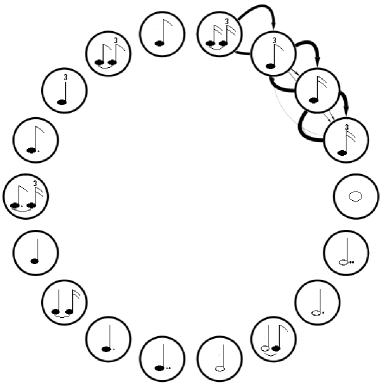
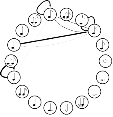
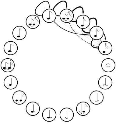
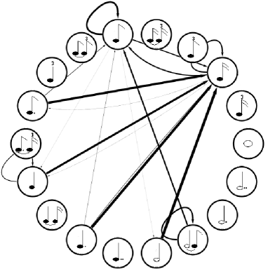
Figure 1: Digraph examples of four music samples: (a) How Blue Can You Get by BB King. (b) Fotografia by Tom Jobim. (c) Is This Love by Bob Marley. (d) From Me To You by The Beatles.

2.3 Feature Extraction

Extracting features is the first step of most pattern recognition systems. Each pattern is represented by its d features or attributes in terms of a vector in a d- dimensional space. In a discrimination problem, the goal is to choose features that allow the pattern vectors belonging to different classes to occupy compact and distinct regions in the feature space, maximizing class separability. After extracting significant features, any classification scheme may be used. In the case of music, features may belong to the main dimensions of it including melody, timbre, rhythm and harmony.

Therefore, one of the main features of this work is to extract features from the digraphs and use them to analyse the complexities of the rhythms, as well as to perform classification tasks. For each sample, a digraph is created as described in the previous section. All digraphs have 18 nodes, corresponding to the quantity of rhythm notation possibilities concerning all the samples, after excluding those that hardly ever happens. This exclusion was important in order to provide an appropriate visual analysis and to better fit the features. In fact, avoiding features that do not significantly contribute to the analysis reduces data dimension, improves the classification performance through a more stable representation and removes redundant or irrelevant information (in this case, minimizes the occurrence of null values in the data matrix).

The features are associated with the weight matrix $W$. As commented in section 2.1, each element in $W$, $w_{ij}$, indicates the weight of the connection from vertex $j$ to $i$, or, in other words, they are meant to represent how often the rhythm notations follow one another in the sample. The weight matrix $W$ has 18 rows and 18 columns. The matrix $W$ is reshaped by a 1 x 324 feature vector. This is done for each one of the genre samples. However, it was observed that some samples even belonging to different genres generated exactly the same weight matrix. These samples were excluded. Thereby, the feature matrix has 280 rows (all non-excluded samples), and 324 columns (the attributes).

An overview of the proposed methodology is illustrated in Figure 2. After extracting the features, a standardization transformation is done to guarantee that the new feature set has zero mean and unit standard deviation. This procedure can significantly improve the resulting classification. Once the normalized features are available, the structure of the extracted rhythms can be analysed by using two different approaches for features analysis: PCA and LDA. We also compare two types of classification methods: Bayesian classifier (supervised) and hierarchical clustering (unsupervised). PCA and LDA are described in section 2.4 and the classification methods are described in section 2.5.

Figure 2: Block diagram of the proposed methodology.

2.4 Feature Analysis and Redundancy Removing

Two techniques are widely used for feature analysis [31, 7, 32]: PCA (Principal Components Analysis) and LDA (Linear discriminant Analysis). Basically, these approaches apply geometric transformations (rotations) to the feature space with the purpose of generating new features based on linear combinations of the original ones, aiming at dimensionality reduction (in the case of PCA) or to seek a projection that best separates the data (in the case of LDA). Figure3 illustrates the basic principles underlying PCA and LDA. The direction $x^{\prime}$ (obtained with PCA) is the best one to represent the two classes with maximum overall dispersion. However, tt can be observed that the densities projected along direction $x^{\prime}$ overlap one another, making these two classes inseparable. Differently, if direction $y^{\prime}$, obtained with LDA, is chosen, the classes can be easily separated. Therefore, it is said that the directions for representation are not always also the best choice for classification, reflecting the different objectives of PCA and LDA. [33]. A.1 and A.2 give more details about these two techniques.

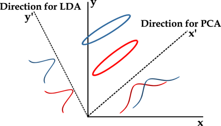
Figure 3: An illustration of PCA (optimizing representation) and LDA projections (optimizing classification), adapted from [33].

2.5 Classification Methodology

Basically, to classify means to assign objects to classes or categories according to the properties they present. In this context, the objects are represented by attributes, or feature vectors. There are three main types of pattern classification tasks: imposed criteria, supervised classification and unsupervised classification. Imposed criteria is the easiest situation in classification, once the classification criteria is clearly defined, generally by a specific practical problem. If the classes are known in advance, the classification is said to be supervised or by example, since usually examples (the training set) are available for each class. Generally, supervised classification involves two stages: learning, in which the features are tested in the training set; and application, when new entities are presented to the trained system. There many approaches involving supervised classification. The current study applied the Bayesian classifier through discriminant functions (B) in order to perform supervised classification. The Bayesian classifier is based on the Bayesian Decision Theory and combines class conditional probability densities (likelihood) and prior probabilities (prior knowledge) to perform classification by assigning each object to the class with the maximum a posteriori probability.

In unsupervised classification, the classes are not known in advance, and there is not a training set. This type of classification is usually called clustering, in which the objects are agglomerated according to some similarity criterion. The basic principle is to form classes or clusters so that the similarity between the objects in each class is maximized and the similarity between objects in different classes minimized. There are two types of clustering: partitional (also called non-hierarchical) and hierarchical. In the former, a fixed number of clusters is obtained as a single partition of the feature space. Hierarchical clustering procedures are more commonly used because they are usually simpler [7, 6, 32, 34]. The main difference is that instead of one definite partition, a series of partitions are taken, which is done progressively. If the hierarchical clustering is agglomerative (also known as bottom-up), the procedure starts with $N$ objects as $N$ clusters and then successively merges the clusters until all the objects are joined into a single cluster (please refer to C for more details about agglomerative hierarchical clustering). Divisive hierarchical clustering (top-down) starts with all the objects as one single cluster, and splits it into progressively finer subclusters.

2.5.1 Performance Measures for Classification

To objectively evaluate the performance of the supervised classification it is necessary to use quantitative criteria. Most used criteria are the estimated classification error and the obtained accuracy. Because of its good statistical properties, as, for example, be asymptotically normal with well defined expressions to estimate its variances, this study also adopted the Cohen Kappa Coefficient [35] as a quantitative measure to analyse the performance of the proposed method. Besides, the kappa coefficient can be directly obtained from the confusion matrix [36] (D), easily computed in supervised classification problems. The confusion matrix is defined as:

$$\centering C=\left[{\begin{array}[]{*{20}c}{c_{11}}&{c_{12}}&\ldots&{c_{1c}}\\ {c_{21}}&\ddots&{}\hfil&\vdots\\ \vdots&{}\hfil&\ddots&{}\hfil\\ {c_{c1}}&\ldots&{}\hfil&{c_{cc}}\\ \end{array}}\right]\@add@centering$$ (1)

where each element $c_{ij}$ represents the number of objects from class $i$ classified as class $j$. Therefore, the elements in the diagonal indicate the number of correct classifications.

3 Results and Discussion

As mentioned before, four musical genres were used in this study: blues, bossa nova, reggae and rock. It was selected music art works from diverse artists, as presented in Tables 2 and 3. Different colors were chosen to represent the genres (color red for genre blues, green for bossa nova, cyan for reggae and pink for rock), in order to provide a better visualization and discussion of the results.

Table 2: Blues and Bossa nova art works

• 	Blues art works
  1	Albert Collins- A Good Fooll
  2	Albert Collins- Fake ID
  3	Albert King- Stormy Monday
  4	Andrews Sister- Boogie Woogie Bugle Boy
  5	B B King- Dont Answer The Door
  6	B B King- Get Off My Back
  7	B B King- Good Time
  8	B B King- How Blue Can You Get
  9	B B King- Sweet Sixteen
  10	B B King- The Thrill Is Gone
  11	B B King- Woke Up This Morning
  12	Barbra Streisand- Am I Blue
  13	Billie Piper- Something Deep Inside
  14	Blues In F For Monday
  15	Bo Diddley- Bo Diddley
  16	Boy Williamson- Dont Start Me Talking
  17	Boy Williamson- Help Me
  18	Boy Williamson- Keep It To Yourself
  19	Buddy Guy- Midnight Train
  20	Charlie Parker- Billies Bounce
  21	Count Basie- Count On The Blues
  22	Cream- Crossroads Blues
  23	Delmore Brothers- Blues Stay Away From Me
  24	Elmore James- Dust My Broom
  25	Elves Presley- A Mess Of Blues
  26	Etta James- At Last
  27	Feeling The Blues
  28	Freddie King- Help Day
  29	Freddie King- Hide Away
  30	Gary Moore- A Cold Day In Hell
  31	George Thorogood- Bad To The Bone
  32	Howlin Wolf- Little Red Rooster
  33	Janis Joplin- Piece Of My Heart
  34	Jimmie Cox- Before You Accuse Me
  35	Jimmy Smith- Chicken Shack
  36	John Lee Hooker- Boom Boom Boom
  37	John Lee Hooker- Dimples
  38	John Lee Hooker- One Bourbon One Scotch One Beer
  39	Johnny Winter- Good Morning Little School Girl
  40	Koko Taylor- Hey Bartender
  41	Little Walter- Juke
  42	Louis Jordan- Let Good Times Roll
  43	Miles Davis- All Blues
  44	Ray Charles- Born To The Blues
  45	Ray Charles- Crying Times
  46	Ray Charles- Georgia On My Mind
  47	Ray Charles- Hit The Road Jack
  48	Ray Charles- Unchain My Heart
  49	Robert Johnson- Dust My Broom
  50	Stevie Ray Vaughan- Cold Shot
  51	Stevie Ray Vaughan- Couldnt Stand The Weather
  52	Stevie Ray Vaughan- Dirty Pool
  53	Stevie Ray Vaughan- Hillbillies From Outer Space
  54	Stevie Ray Vaughan- I Am Crying
  55	Stevie Ray Vaughan- Lenny
  56	Stevie Ray Vaughan- Little Wing
  57	Stevie Ray Vaughan- Looking Out The Window
  58	Stevie Ray Vaughan- Love Struck Baby
  59	Stevie Ray Vaughan- Manic Depression
  60	Stevie Ray Vaughan- Scuttle Buttin
  61	Stevie Ray Vaughan- Superstition
  62	Stevie Ray Vaughan- Tell Me
  63	Stevie Ray Vaughan- Voodoo Chile
  64	Stevie Ray Vaughan- Wall Of Denial
  65	T Bone Walker- Call It Stormy Monday
  66	The Blues Brothers- Everybody Needs Somebody To Love
  67	The Blues Brothers- Green Onions
  68	The Blues Brothers- Peter Gunn Theme
  69	The Blues Brothers- Soulman
  70	W C Handy- Memphis Blues

• 	Bossa nova art works
  71	Antonio Adolfo- Sa Marina
  72	Barquinho
  73	Caetano Veloso- Menino Do Rio
  74	Caetano Veloso- Sampa
  75	Celso Fonseca- Ela E Carioca
  76	Celso Fonseca- Slow Motion bossa nova
  77	Chico Buarque Els Soares- Facamos
  78	Chico Buarque Francis Hime- Meu Caro Amigo
  79	Chico Buarque Quarteto Em Si- Roda Viva
  80	Chico Buarque- As Vitrines
  81	Chico Buarque- Construcao
  82	Chico Buarque- Desalento
  83	Chico Buarque- Homenagem Ao Malandro
  84	Chico Buarque- Mulheres De Athenas
  85	Chico Buarque- Ole O La
  86	Chico Buarque- Sem Fantasia
  87	Chico Buarque- Vai Levando
  88	Dick Farney- Copacaba
  89	Elis Regina- Alo Alo Marciano
  90	Elis Regina- Como Nossos Pais
  91	Elis Regina- Na Batucada Da Vida
  92	Elis Regina- O Bebado E O Equilibrista
  93	Elis Regina- Romaria
  94	Elis Regina- Velho Arvoredo
  95	Emilio Santiago- Essa Fase Do Amor
  96	Emilio Santiago- Esta Tarde Vi Voller
  97	Emilio Santiago- Saigon
  98	Emilio Santiago- Ta Tudo Errado
  99	Gal Costa- Canta Brasil
  100	Gal Costa- Para Machucar Meu Coracao
  101	Gal Costa- Pra Voce
  102	Gal Costa- Um Dia De Domingo
  103	Jair Rodrigues- Disparada
  104	Joao Bosco- Corsario
  105	Joao Bosco- De Frente Para O Crime
  106	Joao Bosco- Jade
  107	Joao Bosco- Risco De Giz
  108	Joao Gilberto- Corcovado
  109	Joao Gilberto- Da Cor Do Pecado
  110	Joao Gilberto- Um Abraco No Bonfa
  111	Luiz Bonfa- De Cigarro Em Cigarro
  112	Luiz Bonfa- Manha De Carnaval
  113	Marcos Valle- Preciso Aprender A Viver So
  114	Marisa Monte- Ainda Lembro
  115	Marisa Monte- Amor I Love You
  116	Marisa Monte- Ando Meio Desligado
  117	Tom Jobim- Aguas De Marco
  118	Tom Jobim- Amor E Paz
  119	Tom Jobim- Brigas Nunca Mais
  120	Tom Jobim- Desafinado
  121	Tom Jobim- Fotografia
  122	Tom Jobim- Garota De Ipanema
  123	Tom Jobim- Meditacao
  124	Tom Jobim- Samba Do Aviao
  125	Tom Jobim- Se Todos Fossem Iguais A Voce
  126	Tom Jobim- So Tinha De Ser Com Voce
  127	Tom Jobim- Vivo Sonhando
  128	Tom Jobim- Voce Abusou
  129	Tom Jobim- Wave
  130	Toquinho- Agua Negra Da Lagoa
  131	Toquinho- Ao Que Vai
  132	Toquinho- Este Seu Olhar
  133	Vinicius De Moraes- Apelo
  134	Vinicius De Moraes- Carta Ao Tom
  135	Vinicius De Moraes- Minha Namorada
  136	Vinicius De Moraes- O Morro Nao Tem Vez
  137	Vinicius De Moraes- Onde Anda Voce
  138	Vinicius De Moraes- Pela Luz Dos Olhos Teus
  139	Vinicius De Moraes- Samba Em Preludio
  140	Vinicius De Moraes-Tereza Da Praia

Table 3: Reggae and Rock art works

• 	Reggae art works
  141	Ace Of Bass- All That She Wants
  142	Ace Of Bass- Dont Turn Around
  143	Ace Of Bass- Happy Nation
  144	Armandinho- Pela Cor Do Teu Olho
  145	Armandinho- Sentimento
  146	Big Mountain- Baby I Love Your Way
  147	Bit Meclean- Be Happy
  148	Bob Marley- Africa Unite
  149	Bob Marley- Buffalo Soldier
  150	Bob Marley- Exodus
  151	Bob Marley- Get Up Stand Up
  152	Bob Marley- I Shot The Sheriff
  153	Bob Marley- Iron Lion Zion
  154	Bob Marley- Is This Love
  155	Bob Marley- Jammin
  156	Bob Marley- No Woman No Cry
  157	Bob Marley- Punky Reggae Party
  158	Bob Marley- Root Rock
  159	Bob Marley- Satisfy
  160	Bob Marley- Stir It Up
  161	Bob Marley- Three Little Birds
  162	Bob Marley- Waiting In The Van
  163	Bob Marley- War
  164	Bob Marley- Wear My
  165	Bob Marley- Zimbabwe
  166	Cidade Negra- A Cor Do Sol
  167	Cidade Negra- A Flexa E O Vulcao
  168	Cidade Negra- A Sombra Da Maldade
  169	Cidade Negra- Aonde Voce Mora
  170	Cidade Negra- Eu Fui Eu Fui
  171	Cidade Negra- Eu Tambem Quero Beijar
  172	Cidade Negra- Firmamento
  173	Cidade Negra- Girassol
  174	Cidade Negra- Ja Foi
  175	Cidade Negra- Mucama
  176	Cidade Negra- O Ere
  177	Cidade Negra- Pensamento
  178	Dazaranhas- Confesso
  179	Dont Worry
  180	Flor Do Reggae
  181	Inner Circle- Bad Boys
  182	Inner Circle- Sweat
  183	Jimmy Clif- I Can See Clearly Now
  184	Jimmy Clif- Many Rivers To Cross
  185	Jimmy Clif- Reggae Night
  186	Keep On Moving
  187	Manu Chao- Me Gustas Tu
  188	Mascavo- Anjo Do Ceu
  189	Mascavo- Asas
  190	Natiruts- Liberdade Pra Dentro Da Cabeca
  191	Natiruts- Presente De Um Beija Flor
  192	Natiruts- Reggae Power
  193	Nazarite Skank
  194	Peter Tosh- Johnny B Goode
  195	Shaggy- Angel
  196	Shaggy- Bombastic
  197	Shaggy- It Wasnt Me
  198	Shaggy- Strenght Of A Woman
  199	Sublime- Badfish
  200	Sublime- D Js
  201	Sublime- Santeria
  202	Sublime- Wrong Way
  203	Third World- Now That We Found Love
  204	Tribo De Jah- Babilonia Em Chamas
  205	Tribo De Jah- Regueiros Guerreiros
  206	Tribo De Jah- Um So Amor
  207	U B40- Bring Me Your Cup
  208	U B40- Home Girl
  209	U B40- To Love Somebody
  210	Ub40- Red Red Wine

• 	Rock art works
  211	Aerosmith- Kings And Queens
  212	Aha- Stay On These Roads
  213	Aha- Take On Me
  214	Aha- Theres Never A Forever Thing
  215	Beatles- Cant Buy Me Love
  216	Beatles- From Me To You
  217	Beatles- I Want To Hold Your Hand
  218	Beatles- She Loves You
  219	Billy Idol- Dancing With Myself
  220	Cat Steves- Another Saturday Night
  221	Creed- My Own Prison
  222	Deep Purple- Deamon Eye
  223	Deep Purple- Hallelujah
  224	Deep Purple- Hush
  225	Dire Straits- Sultan Of Swing
  226	Dire Straits- Walk Of Life
  227	Duran Duran- A View To A Kill
  228	Eric Clapton- Cocaine
  229	Europe- Carrie
  230	Fleetwood Mac- Dont Stop
  231	Fleetwood Mac- Dreams
  232	Fleetwood Mac- Gold Dust Woman
  233	Foo Fighters- Big Me
  234	Foo Fighters- Break Out
  235	Foo Fighters- Walking After You
  236	Men At Work- Down Under
  237	Men At Work- Who Can It Be Now
  238	Metallica- Battery
  239	Metallica- Fuel
  240	Metallica- Hero Of The Day
  241	Metallica- Master Of Puppets
  242	Metallica- My Friendof Misery
  243	Metallica- No Leaf Clover
  244	Metallica- One
  245	Metallica- Sad But True
  246	Pearl Jam- Alive
  247	Pearl Jam- Black
  248	Pearl Jam- Jeremy
  249	Pet Shop Boys- Go West
  250	Pet Shop Boys- One In A Million
  251	Pink Floyd- Astronomy Domine
  252	Pink Floyd- Have A Cigar
  253	Pink Floyd- Hey You
  254	Queen- Another One Bites The Dust
  255	Queen- Dont Stop Me Now
  256	Queen- I Want It All
  257	Queen- Play The Game
  258	Queen- Radio Gaga
  259	Queen- Under Pressure
  260	Red Hot Chilli Pepers- Higher Ground
  261	Red Hot Chilli Pepers- Otherside
  262	Red Hot Chilli Pepers- Under The Bridge
  263	Rolling Stones- Angie
  264	Rolling Stones- As Tears Go By
  265	Rolling Stones- Satisfaction
  266	Rolling Stones- Street Of Love
  267	Steppen Wolf- Magic Carpet Ride
  268	Steve Winwood- Valerie
  269	Steve Winwood- While You See A Chance
  270	Tears For Fears- Shout
  271	The Doors- Hello I Love You
  272	The Doors- Light My Fire
  273	The Doors- Love Her Madly
  274	U2- Elevation
  275	U2- Ever Lasting Love
  276	U2- When Love Comes To Town
  277	Van Halen- Dance The Night Away
  278	Van Halen- Dancing With The Devil
  279	Van Halen- Jump
  280	Van Halen- Panama

Once we want to reduce data dimensionality, it is necessary to set the suitable number of principal components that will represent the new features. Not surprisingly, in a high dimensional space the classes can be easily separated. On the other hand, high dimensionality increases complexity, making the analysis of both extracted features and classification results a difficult task. One approach to get the ideal number of principal components is to verify how much of the data variance is preserved. In order to do so, the $l$ first eigenvalues ($l$ is the quantity of principal components to be verified) are summed up and the result is divided by the the sum of all the eigenvalues. If the result of this calculation is a value equal or greater than 0.75, it is said that these number of components (or new features) preserves at least 75% of the data variance, which is often enough for classification purposes. When PCA was applied to the normalized rythm features, as illustrated in Figure 4, it was observed that 20 principal components preserved 76% of the variance of the data. That is, it is possible to reduce the data dimensionality from 364-D to 20-D without a significant loss of information. Nevertheless, as will be shown in the following, depending on the classifier and how the classification task was performed, different number of components were required in each situation in order to achieve suitable results. Despite the fact of preserving only 32% of the variance, Figure 4 shows the first three principal components, that is, the first three new features obtained with PCA. Figure 4 shows the first and second features and Figure 4 shows the first and third features. It is noted that the classes are completely overlapped, making the problem of automatic classification a nontrivial task.

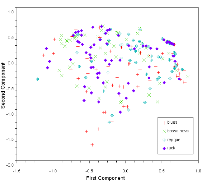
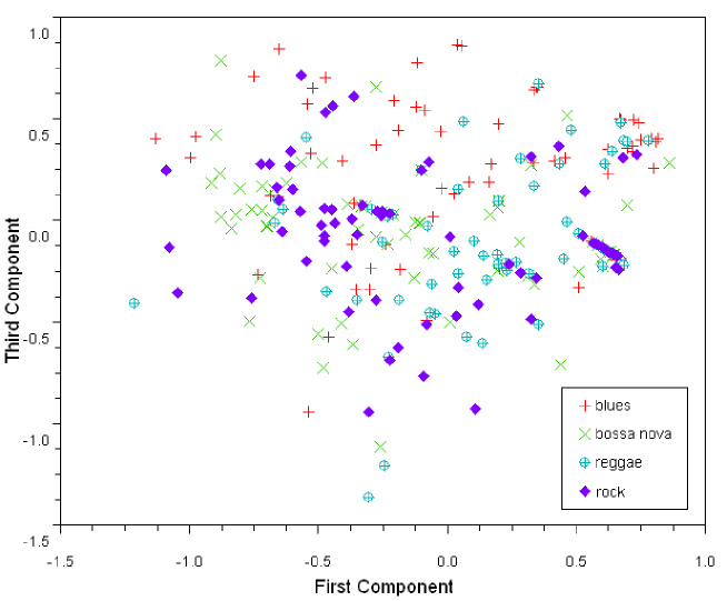
Figure 4: The new first three feaures obtained by PCA. (a) First and second axes. (b) First and third axes.

In all the following supervised classification tasks, re-substitution means that all objects from each class were used as the training set (in order to estimate the parameters) and all objects were used as the testing set. Hold-out 70%-30% means that 70% of the objects from each class were used as the training set and 30% (different ones) for testing. Finally, in hold-out 50%-50%, the objects were separated into two groups: 50% for training and 50% for testing.

The kappa variance is strongly related to its accuracy, that is, how reliable are its value. The higher is its variance, the lower is its accuracy. Once the kappa coefficient is a statistics, in general, the use of large datasets improves its accuracy by making its variance smaller. This concept can be observed in the results. The smaller variance occurred in the re-substitution situation, in which all samples constitute the testing set. This indicates that re-substitution provided the best kappa accurary in the experiments. On the other hand, hold-out 70%-30% provided the higher kappa variance, once only 30% of the samples establishes the testing set.

The results obtained by the Quadratic Bayesian Classifier using PCA are shown in Table 4 in terms of kappa, its variance, the accurary of the classification and the overall performance according to the value of kappa.

Table 4: PCA kappa and accuracy for the Quadratic Bayesian Classifier

	Kappa	Variance	Accuracy	Performance
Re-Substitution	0.66	0.0012	74.65%	Substantial
Hold-Out (70%-30%)	0.23	0.0057	42.5%	Fair
Hold-Out (50%-50%)	0.22	0.0033	41.43%	Fair

Table 4 also indicates that the performance was not satisfactory for the Hold-Out (70%-30%) and Hold-Out (50%-50%). As the PCA is a not supervised approach, the parameter estimation performance (of covariance matrices for instance) is strongly degraded because of the small sample size problem.

The confusion matrix for the re-substitution classification task in Table 4 is illustrated in Table 5. All reggae samples were classified correctly. In addition, many samples from the other classes were classified as reggae.

Table 5: Confusion Matrix for the Quadratic Bayesian Classifier using PCA and Re-Substitution

	Blues	Bossa nova	Reggae	Rock
Blues	48	0	22	0
Bossa nova	2	47	21	0
Reggae	0	0	70	0
Rock	1	1	24	44

Table 6 presents the misclassified art works of the confusion matrix in Table 5.

Table 6: Misclassified art works using PCA with Quadratic Bayesian Classifier and Re-Substitution

Blues as Reggae	3 6 10 12 16 17 18 23 25 28 34 36 37 38 40 51 52 54 56 58 63 69
Bossa nova as Blues	123 126
Bossa nova as Reggae	74 82 83 86 89 96 97 98 100 103 104 105 106 107 109 112 114 115 117 118 125
Rock as Blues	266
Rock as Bossa nova	212
Rock as Reggae	217 219 226 228 231 233 236 237 239 245 247 249 254 255 257 261 262 264 267 273 274 275 276 278

With the purpose of comparing two different classifiers, the obtained results by the Linear Bayesian Classifier using PCA are shown in Table 7, again, in terms of kappa, its variance, the accurary of the classification and the overal performance according to its value. The performance of the Hold-Out (70%-30%) and Hold-Out (50%-50%) classification task increased slightly, mainly due to the fact that here a unique covariance matrix is estimated using all the samples in the dataset.

Table 7: PCA kappa and accuracy for the Linear Bayesian Classifier

	Kappa	Variance	Accuracy	Performance
Re-Substitution	0.63	0.0013	72.15%	Substantial
Hold-Out (70%-30%)	0.35	0.0055	51.25%	Fair
Hold-Out (50%-50%)	0.31	0.0032	48.58%	Fair

Figure 5 depicts the value of kappa depending on the quantity of principal components used in the Quadratic and Linear Bayesian Classifier. The last value of each graphic makes it clear that from this value onwards the classification can not be done due to singularity problems involving the inversion of the covariance matrices (curse of dimensionality). It can be observed that this singularity threshold is different in each situation. However, for the quadratic classifier this value is in the range of about 40-55 components; while, for the linear classifier, is in the range of about 86-115 components. The smaller quantity for the quadratic classifier can be explained by the fact that there are four covariance matrices, each one estimated from the samples for one respective class. As there are 70 samples in each class, singularity problems will occur in a smaller dimensional space when compared to the linear classifier, that uses all the 280 samples to estimate one unique covariance matrix. Therefore, the ideal number of principal components allowing the highest value of kappa should be those circled in red in Figure 5.

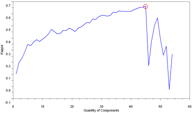
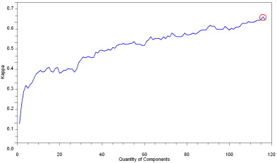
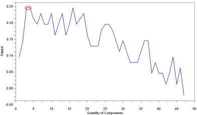
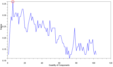
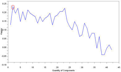
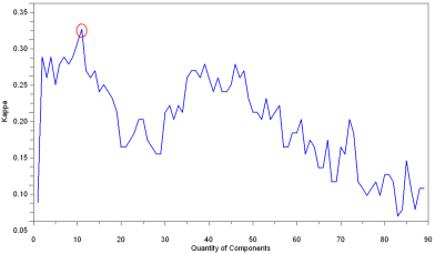
Figure 5: Values of Kappa varying the number of principal components (a)Quadratic Bayesian Classifier: Re-Substitution (b)Linear Bayesian Classifier: Re-Substitution (c)Quadratic Bayesian Classifier: Hold-Out (70%-30%) (d)Linear Bayesian Classifier: Hold-Out (70%-30%) (e)Quadratic Bayesian Classifier: Hold-Out (50%-50%) (f)Linear Bayesian Classifier: Hold-Out (50%-50%).

Keeping in mind that the problem of automatic genre classification is a nontrivial task, that in this study only one aspect of the rhythm is been analysed (the occurrence of the ryhthm notations), and that PCA is an unsupervised approach for feature extraction, the correct classifications presented in Tables 4 and 7 for the re-substitution situation corroborate strongly the viability of the proposed methodology. In spite of the complexity of comparing differents proposed approaches to automatic genre classification discussed in the Introduction, these accuracy values are very close or even superior when compared to previous works [10, 11, 12, 15, 3].

Similarly, Figure 6 shows the three components, namely the three new features obtained with LDA. As mentioned before, LDA approach has a restriction of obtaining only $C-1$ nonzero eigenvalues, where $C$ is the number of class. Therefore, only three components are computed. Once it is a supervised approach and the main goal is to maximize class separability, the four classes in Figure 6 and Figure 6 are clearer than in PCA, although still involving substantial overlaps. This result corroborates that automatic classification of musical genres is not a trivial task.

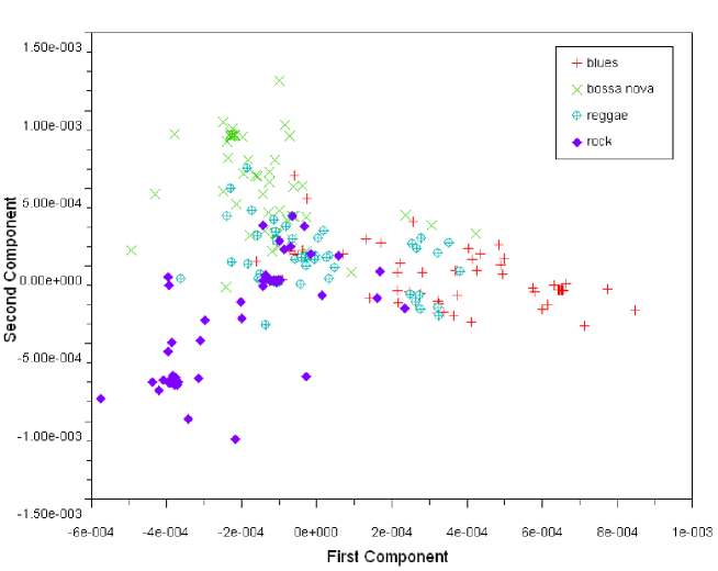
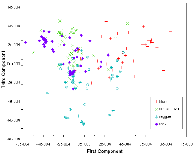
Figure 6: The new first three feaures obtained by LDA. (a) First and second features. (b) First and third features.

Table 8 presents the results obtained by the Quadratic Bayesian Classifer using LDA. Differently from PCA, the use of hold-out (70%-30%) and hold-out (50%-50%) provided good results, what is notable and reflects the supervised characteristic of LDA, which makes use of all discriminant information available in the feature matrix.

Table 8: LDA kappa and accuracy for the Quadratic Bayesian Classifier

	Kappa	Variance	Accuracy	Performance
Re-Substitution	0.66	0.0012	74.29%	Substantial
Hold-Out (70%-30%)	0.62	0.0045	71.25%	Substantial
Hold-Out (50%-50%)	0.64	0.0025	72.86%	Substantial

Despite the value of kappa and its variance being the same using LDA with re-substitution and PCA with re-substitution, the two confusion matrix are strongly distinct each other. In the first case, demostrated in Table 9, the misclassified art works are well distributed among the four classes, while with PCA (Table 5) they are concentrated in one class, represented by the reggae genre. The results obtained with LDA technique are particularly promising because they reflect the nature of the data. Although widely used, terms such as rock, reggae or pop often remain loosely defined [3]. Yet, it is worthwhile to remember that the intensity of the beat, which is a very important aspect of the rhythm has not been considered in this work. This means that analysing rhythm only through notations, as currently proposed, could poise difficulties even for human experts. These misclassified art works have similar properties described in terms of rhythm notations and, as a result, they generate similar weight matrices. Therefore, the proposed methodology, although requiring some complementations, seems to be a significant contribution towards the development of viable alternative approach to automatic genre classification.

Table 9: Confusion Matrix for the Quadratic Bayesian Classifier using LDA and Re-Substitution

	Blues	Bossa nova	Reggae	Rock
Blues	58	6	4	2
Bossa nova	3	52	7	8
Reggae	8	8	44	10
Rock	4	7	5	54

The misclassified art works of the confusion matrix in Table 9 are identified in Table 10.

Table 10: Misclassified art works using LDA with Quadratic Bayesian Classifier and Re-Substitution

Blues as Bossa nova	2 30 52 54 58 63
Blues as Reggae	5 17 28 69
Blues as Rock	6 51
Bossa nova as Blues	79 80 116
Bossa nova as Reggae	90 96 97 105 112 122 131
Bossa Bova as Rock	76 78 83 98 100 103 107 109
Reggae as Blues	144 152 166 170 188 190 193 203
Reggae as Bossa nova	158 159 162 164 169 181 197 208
Reggae as Rock	146 156 157 160 168 175 180 189 198 210
Rock as Blues	238 239 245 278
Rock as Bossa nova	233 237 254 262 264 266 276
Rock as Reggae	219 228 255 261 263

The results for the Linear Bayesian Classifier using LDA are shown in Table 11. In fact, they are closely similar to those obtained by the Quadratic Bayesian Classifier (Table 8).

Table 11: LDA kappa and accuracy for the Linear Bayesian Classifier

	Kappa	Variance	Accuracy	Performance
Re-Substitution	0.65	0.0012	73.58%	Substantial
Hold-Out (70%-30%)	0.63	0.0043	72.5%	Substantial
Hold-Out (50%-50%)	0.64	0.0025	72.86%	Substantial

As mentioned in section A.2, linear discriminant analysis also allows us to quantify the intra and interclass dispersion of the feature matrix through functionals such as the trace and determinant computed from the scatter matrices [37]. The overall intraclass scatter matrix, hence $S_{intra}$; the intraclass scatter matrix for each class, hence $S_{intraBlues}$, $S_{intraBossaNova}$, $S_{intraReggae}$ and $S_{intraRock}$; the interclass scatter matrix, hence, $S_{inter}$; and the overall separability index, hence $\left(S_{intra}^{-1}*S_{inter}\right)$, were computed. Their respective traces are:

$trace(S_{intra})$ =   499.526

$trace(S_{intraBlues})$ =   138.615

$trace(S_{intraBossaNova})$ =   119.302

$trace(S_{intraReggae})$ =   98.327

$trace(S_{intraRock})$ =   143.280

$trace(S_{inter})$ =   21.598

$trace\left(S_{intra}^{-1}*S_{inter}\right)$ =   3.779

Two important observations are worth mentioning. First, these traces emphasise the difficulty of this classification problem: the traces of the intraclass scatter matrices are too high, and the trace of the interclass scatter matrix together with the overal separability index, too small. This confirms that the four classes are overlapping completely. Second, the smaller intraclass trace is related to the reggae genre (it is the most compact class). This may justify why in the experiments art works belonging to reggae were more frequently 90%-100% correctly classified.

The PCA and LDA approaches help to identify which features contribute the most to the classification. This is an interesting analysis that can be performed by verifying the strength of each element in the first eigenvectors, and then associating those elements with the original features. Within the current study, it was figured out that the first ten sequences of rhythm notations that most contributed to separation correspond to those illustrated in Figure 7. In the case of the first and second eigenvectors obtained by PCA and LDA, the ten elements with higher values were selected, and the indices of these elements were associated with the sequences in the original weight matrix. Figure 7 and 7 shows the resulting sequences according to the first and second eigenvectors of PCA. The thickness of the edges is set by the value of the corresponding element in the eigenvector. It is interesting that these sequences are those that mostly frequently happen in the rhythms from all four genres studied here. That is, they correspond to the elements that play the greatest role in representing the rhythms. Therefore, it can be said that these are the ten most representative sequences, when the first and second eigenvectors of PCA are taken into account. Triples of eighth and sixteenth notes are particularly important in blues and reggae genres. Similarly, Figure 7 and Figure 7 show the resulting sequences according to the first and second eigenvectors of LDA. Differently from those obtained by PCA, these sequences are not common to all the rhythms, but they must happen with distinct frequency within each genre. Thus, they are referred here as the ten most discriminative sequences, when the first and second eigenvectors of LDA are taken into account.

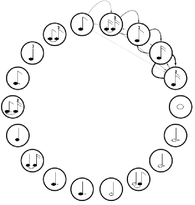
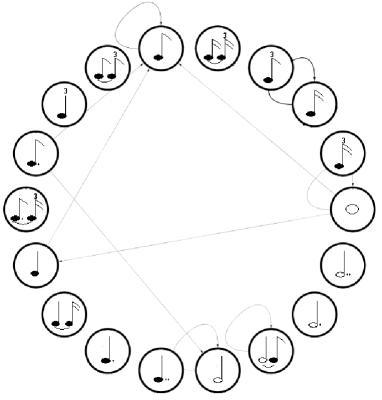
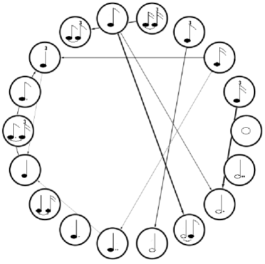
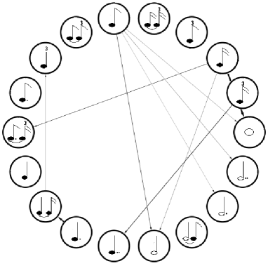
Figure 7: Ten most significant sequences of rhythm notations according to: (a) PCA first eigenvector (b) PCA second eigenvector (c) LDA first eigenvector (d) LDA second eigenvector

Clustering results are discussed in the following. The number of clusters was defined as being four, in order to provide a fair comparison with the supervised classification results. The idea of the confusion matrix in Table 12 is to verify how many art works from each class were placed in each one of the four clusters. For example, it is known that art works from one to seventy belongs to the blues genre. Then, the first line of this confusion matrix indicates that four blues art works were placed in the cluster one, thirty three in the cluster two, seven in the cluster three and twenty six in the cluster four. It can also be observed that in cluster one reggae art works are the majority (nineteen), despite the small difference with the number of rock art works (fifteen); while in cluster two the majority are blues art works; in cluster three the majority are rock art works; and in cluster four the majority are bossa nova art works.

Table 12: Confusion Matrix for the Agglomerative Hierarchical Clustering

	Classe 1	Classe 2	Classe 3	Classe 4
Classe 1	4	33	7	26
Classe 2	9	4	7	50
Classe 3	19	15	6	30
Classe 4	15	5	14	36

Comparing the confusion matrix in Table 12 and the confusion matrix for the Quadradic Bayesian Classifier using PCA in Table 5, it is interesting to notice that: in the former, the cluster four contains considerable art works from the four genres (twenty six from blues, fifty from bossa nova, thirty from reggae and thirty six from rock), in a total of one hundred forty two art works; in the later, a considerable number of art work from blues (twenty two), bossa nova (twenty one) and rock (twenty four) were misclassified as reggae, in a total of one hundred thirty seven art works belonging this class. This means that the PCA representation was not efficient in discriminating reggae from the other genres, while cluster four was the one that mostly intermixed art works from all classes.

Figure 8 presents the dendrogram with the four identified clusters. Different colors were used for the sake of enhanced visual analysis. Cluster one is colored in green, cluster two in pink, cluster three in red, and cluster four in cyan. These colors were based on the dominant class in each cluster. For example, cluster one is colored in green because bossa nova art works are majority in this cluster.

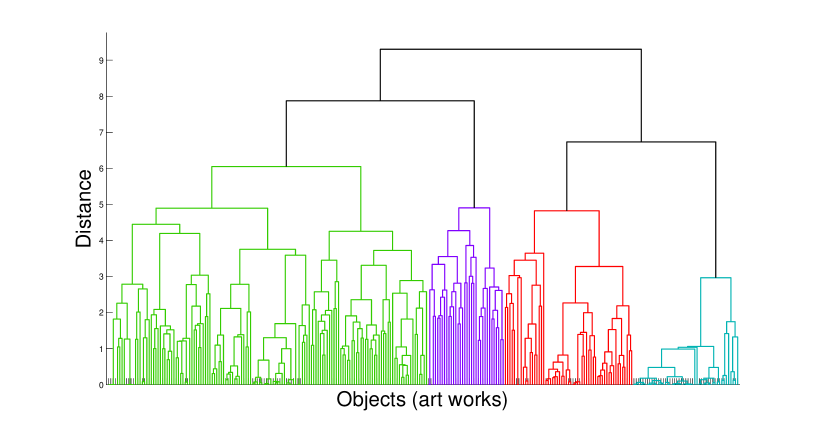
Figure 8: The dendrogram of the resulting four clusters (colored in green, pink, red and cyan.

The four obtained clusters are detailed in Figures 9 to 12, in which the legends presents the grouped art works from each cluster (blues art works are in red, bossa nova art works are in green, reggae art works in cyan and rock art works in pink).

As a consequence of working in a higher dimension feature space, the agglomerative hierarquical clustering approach could better separate the data when compared to the PCA and LDA-based approaches, which are applied over a projected version of the original measurements.

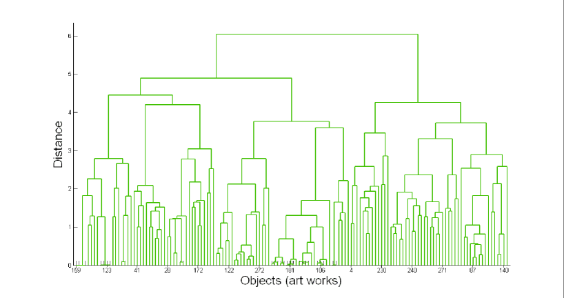
Figure 9: The detailed dendrogram for cluster in green. The objects were specified here, from left to right: 159 237 158 74 37 80 132 85 117 208 123 126 2 78 39 23 62 45 138 11 41 156 46 88 114 131 164 266 166 258 28 174 105 233 141 167 184 81 163 207 172 182 248 72 95 216 13 185 96 112 122 111 98 175 209 266 177 247 212 206 272 179 225 253 52 54 63 89 262 86 181 254 276 58 118 264 197 115 116 82 106 125 169 220 119 134 162 243 250 201 4 15 199 14 53 57 93 244 242 165 230 265 232 19 55 136 104 238 215 251 240 252 241 269 60 195 68 148 277 280 271 101 110 268 137 186 22 30 71 73 87 108 121 130 129 133 113 135 124 127 140 and 221.

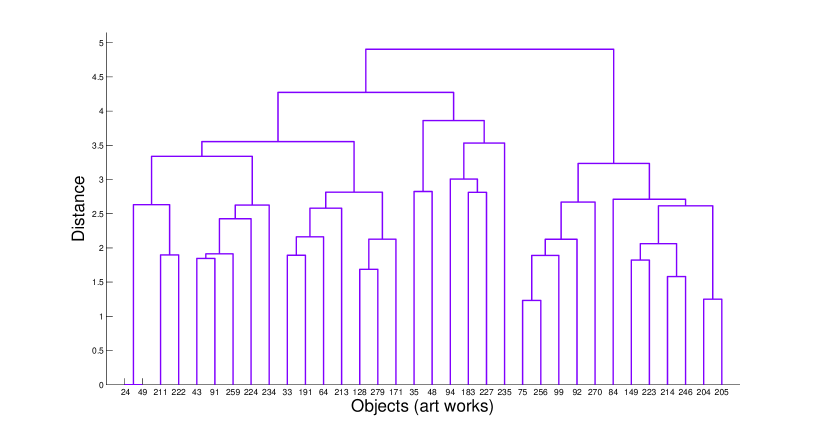
Figure 10: The detailed dendrogram for cluster in pink.The objects were specified here, from left to right: 24 49 211 222 43 91 259 224 234 33 191 64 213 128 279 171 35 48 94 183 227 235 75 256 99 92 270 84 149 223 214 246 204 and 205

.

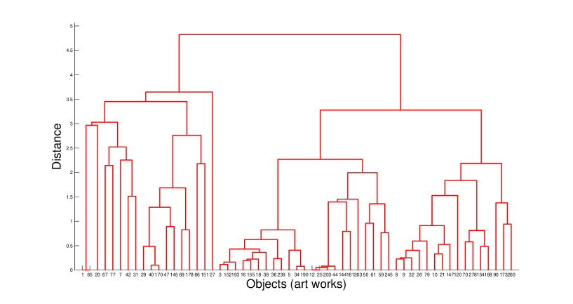
Figure 11: The detailed dendrogram for cluster in red.The objects were specified here, from left to right: 1 65 20 67 77 7 42 31 29 40 170 47 145 69 178 66 151 27 3 152 193 16 155 18 38 36 239 5 34 190 12 25 203 44 144 161 263 50 61 59 245 8 9 32 26 79 10 21 147 120 70 278 154 188 90 173 and 260.

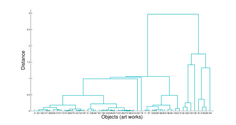
Figure 12: The detailed dendrogram for cluster in cyan. The objects were specified here, from left to right: 6 231 160 157 189 200 107 217 274 168 275 142 153 187 51 236 267 83 100 143 249 257 103 146 273 180 210 102 176 17 97 109 228 198 255 196 261 192 219 56 202 150 139 76 218 229 and 194.

4 Concluding Remarks

Automatic music genre classification has become a fundamental topic in music research since genres have been widely used to organize and describe music collections. They also reveal general identities of different cultures. However, music genres are not a clearly defined concept so that the development of a non-controversial taxonomy represents a challenging, non-trivial taks.

Generally speaking, music genres summarize common characteristics of musical pieces. This is particular interesting when it is used as a resource for automatic classification of pieces. In the current paper, we explored genre classification while taking into account the musical temporal aspects, namely the rhythm. We considered pieces of four musical genres (blues, bossa nova, reggae and rock), which were extracted from MIDI files and modeled as networks. Each node corresponded to one rhythmc notation, and the links were defined by the sequence in which they occurred along time. The idea of using static nodes (nodes with fixed positions) is particularly interesting because it provides a primary visual identification of the differences and similarities between the rythms from the four genres. A Markov model was build from the networks, and the dynamics and dependencies of the rhythmic notations were estimated, comprising the feature matrix of the data. Two different approaches for features analysis were used (PCA and LDA), as well as two types of classification methods (Bayesian classifier and hierarchical clustering).

Using only the first two principal componentes, the different types of rhythms were not separable, although for the first and third axes we could observe some separation between three of the classes (blues, bossa nova and reggae), while only the samples of rock overlapped the other classes. However, taking into account that twenty components were necessary to preserve 76% of the data variance, it would be expected that only two or three dimensions would not be sufficient to allow suitable saparability. Notably, the dimensionality of the problem is high, that is, the rhythms are very complex and many dimensions (features) are necessary to separate them. This is one of the main findings of the current work. With the help of LDA analysis, another finding was reached which supported the assumption that the problem of automatic rhythm classification is no trivial task. The projections obtained by considering the first and second, and first and third axes implied in better discrimination between the four classes than that obtained by the PCA.

Unlike PCA and LDA, agglomerative hierarchical clustering works on the original dimensions of the data. The application of the methodology led to a substantially better discrimination, which provides a strong evidence of the complexity of the problem studied here. The results are promising in the sense that in each cluster is dominated by a different genre, showing the viability of the proposed approach.

It is clear from our study that musical genres are very complex and present redundancies. Sometimes it is difficult even for an expert to distinguish them. This difficulty becomes more critical when only the rhythm is taken into account.

Several are the possibilities for future research implied by the reported investigation. First, it would be interesting to use more measurements extracted from rhythm, especially the intensity of the beats, as well as the distribution of instruments, which is poised to improve the classification results. Another promising venue for further investigation regards the use of other classifiers, as well as the combination of results obtained from ensemble of distinct classifiers. In addition, it would be promising to apply multi-labeled classification, a growing field of research in which non-disjointed samples can be associated to one or more labels [38]. Nowadays, multi-labeled classification methods have been increasingly required by applications such as text categorization [39], scene classification [40], protein classification [41], and music categorization in terms of emotion [42], among others. The possibility of multigenres classification is particularly promising and probably closer to the human experience. Another interesting future work is related to the synthesis of rhythms. Once the rhythmic networks are available, new rhythms with similar characteristics according to the specific genre can be artificially generated.

5 Acknowledgments

Debora C Correa is grateful to FAPESP (2009/50142-0) for financial support and Luciano da F. Costa is grateful to CNPq (301303/06-1 and 573583/2008-0) and FAPESP (05/00587-5) for financial support.

Appendices

Appendix A Multivariate Statistical Methods

A.1 Principal Component Analysis

Principal Component Analysis is a second order unsupervised statistical technique. By second order it is meant that all the necessary information is available directly from the covariance matrix of the mixture data, so that there is no need to use the complete probability distributions. This method uses the eigenvalues and eigenvectors of the covariance matrix in order to transform the feature space, creating orthogonal uncorrelated features. From a multivariate dataset, the principal aim of PCA is to remove redundancy from the data, consequently reducing the dimensionality of the data. Additional information about PCA and its relation to various interesting statistical and geometrical properties can be found in the pattern recognition literature, e.g. [43, 32, 7, 6].

Consider a vector x with n elements representing some features or measurements of a sample. In the first step of PCA transform, this vector x is centered by subtracting its mean, so that $\textbf{x}\leftarrow\textbf{x}-E\left\{\textbf{x}\right\}$. Next, x is linearly transformed to a different vector y which contains m elements, m $<$ n, removing the redundancy caused by the correlations. This is achieved by using a rotated orthogonal coordinate system in such a way that the elements in x are uncorrelated in the new coordinate system. At the same time, PCA maximizes the variances of the projections of x on the new coordinate axes (components). These variances of the components will differ in most applications. The axes associated to small dispersions (given by the respectively associated eigenvalues) can be discarded without losing too much information about the original data.

A.2 Linear discriminant Analysis

Linear discriminantAnalysis (LDA) can be considered a generalization of Fisher’s Linear discriminant Function for the multivariate case [7, 32]. It is a supervised approach that maximizes data separability, in terms of a simililarity criterion based on scatter matrices. The basic idea is that objects belonging to the same class are as similar as possible and objects belonging to distinct classes are as different as possible. In other words, LDA looks for a new, projected, feature space where that maximizes interclass distance while minimizing the intraclass distance. This result can be later used for linear classification, and it is also possible to reduce dimensionality before the classification task. The scatter matrix for each class indicates the dispersion of the features vectors within the class. The intraclass scatter matrix is defined as the sum of the scatter matrices of all classes and expresses the combined dispersion in each class. The interclass scatter matrix quantifies how disperse the classes are, in terms of the position of their centroids.

It can be shown that the maximization criterion for class separability leads to a generalized eigenvalue problem ([32, 7]). Therefore, it is possible to compute the eigenvalues and eigenvectors of the matrix defined by $\left(S_{intra}^{-1}*S_{inter}\right)$, where $S_{intra}$ is the intraclass scatter matrix and $S_{inter}$ is the interclass scatter matrix. The m eigenvectors associated to the m largest eigenvalues of this matrix can be used to project the data. However, the rank of $\left(S_{intra}^{-1}*S_{inter}\right)$ is limited to $\textit{C}-1$, where C is the number of classes. As a consequence, there are $\textit{C}-1$ nonzero eigenvalues, that is, the number of new features is conditioned to the number of classes, $\textit{m}\leq\textit{C}-1$. Another issue is that, for high dimensional problems, when the number of available training samples is smaller than the number of features, $S_{intra}$ becomes singular, complicating the generalized eigenvalue solution.

More information about the LDA is [31, 33, 7, 32].

Appendix B Linear and Quadratic Discriminant Functions

If normal distribution over the data is assumed, it is possible to state that:

$$p\left(x|\omega_{i}\right)=\frac{1}{\left(2\pi\right)^{\frac{d}{2}}\left|\Sigma\right|^{\frac{1}{2}}}\exp\left\{-\frac{1}{2}\left(\vec{x}-\vec{\mu}\right)^{T}\Sigma^{-1}\left(\vec{x}-\vec{\mu}\right)\right\}$$ (2)

The components of the parameter vector for class $j$, $\vec{\theta}_{j}=\left\{\vec{\mu}_{j},\Sigma_{j}\right\}$, where $\vec{\mu}_{j}$ and $\Sigma_{j}$ are the mean vector and the covariance matrix of class $j$, respectively, can be estimated by maximum likelihood as follows:

$$\hat{\vec{\mu}}_{j}=\frac{1}{N}\sum_{i=1}^{N}\vec{x}_{i}$$ (3)

$$\hat{\vec{\Sigma}}_{j}=\frac{1}{N}\sum_{i=1}^{N}\left(\vec{x}_{i}-\vec{\mu}_{i}\right)\left(\vec{x}_{i}-\vec{\mu}_{i}\right)^{T}$$ (4)

Within this context, classification can be achieved with discriminant functions, $g_{i}$, assigning an observed pattern vector $\vec{x}_{i}$ to the class $\omega_{j}$ with the maximum discriminant function value. By using Bayes’s rule, not considering the constant terms, and using the estimated parameters above, a decision rule can be defined as: assign an object $\vec{x}_{i}$ to class $\omega_{j}$ if $g_{j}>g_{i}$ for all $i\neq j$, where the discriminantfunction $g_{i}$ is calculated as:

$$g_{i}\left(\vec{x}\right)=\log\left(p\left(\omega_{i}\right)\right)-\frac{1}{2}\log\left(\left|\hat{\Sigma}_{i}\right|\right)-\frac{1}{2}\left(\vec{x}-\hat{\vec{\mu}}_{j}\right)^{T}\hat{\Sigma}_{i}^{-1}\left(\vec{x}-\hat{\vec{\mu}}_{j}\right)$$ (5)

Classifying an object or pattern $\vec{x}$ on the basis of the values of $g_{i}\left(\vec{x}\right)$, $i=1,...,C$ ($C$ is the number of classes), with estimated parameters, defines a quadratic discriminant classifier or quadratic Bayesian classifier or yet quadratic Gaussian classifier [32].

The prior probability, $p\left({\omega_{i}}\right)$, can be simply estimated by:

$$p\left({\omega_{i}}\right)=\frac{{n_{i}}}{{\sum\nolimits_{j}{n_{j}}}}$$ (6)

where $n_{i}$ is the number of samples of class $\omega_{i}$.

In multivariate classification situations, with different covariance matrices, problems may occur in the quadratic Bayesian classifier when any of the matrices $\hat{\Sigma}_{i}$ is singular. This usually happens when there are not enough data to obtain efficient estimative for the covariance matrices $\Sigma_{i}$, $i=1,2,...,C$. An alternative to minimize this problem consist of estimating one unique covariance matrix over all classes, $\hat{\Sigma}=\hat{\Sigma}_{1}=...=\hat{\Sigma}_{C}$. In this case, the discriminantfunction becomes linear in $\vec{x}$ and can be simplified:

$$g_{i}\left(\vec{x}\right)=log\left(p\left(\omega_{i}\right)\right)-\frac{1}{2}\hat{\vec{\mu}}_{i}^{T}\hat{\Sigma}^{-1}\hat{\vec{\mu}}_{i}+\vec{x}^{T}\hat{\Sigma}^{-1}\hat{\vec{\mu}}_{i}$$ (7)

where $\hat{\Sigma}$ is the covariance matrix, common to all classes. The classification rule remains the same. This defines a linear discriminant classifier (also known as linear Bayesian classifier or linear Gaussian classifier) [32].

Appendix C Agglomerative Hierarchical Clustering

Agglomerative hierarchical clustering groups progressively the $N$ objects into $C$ classes according to a defined parameter. The distance or similarity between the feature vectors of the objects are usually taken as such parameter. In the first step, there is a partition with $N$ clusters, each cluster containing one object. The next step is a different partition, with $N-1$ clusters, the next a partition with $N-2$ clusters, and so on. In the $n$th step, all the objects form a unique cluster. This sequence groups objects that are more similar to one another into subclasses before objects that are less similar. It is possible to say that, in the $k$th step, $C=N-k+1$.

To show how the objects are grouped, hierarchical clustering can be represented by a corresponding tree, called dendrogram. Figure 13 illustrates a dendrogram representing the results of hierarchical clustering for a problem with eight objects. The measure of similarity among clusters can be observed in the vertical axis. The different number of classes can be obtained by horizontally cutting the dendrogram at different values of similarity or distance.

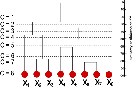
Figure 13: A dendrogram for a simple situation involving eight objects, adapted from [7].

Hence, to perform hierarchical cluster analysis it is necessary to define three main parameters. The first regards how to quantify the similarity between every pair of objects in the data set, that is, how to calculate the distance between the objects. Euclidean distance, which is frequently used, will be adopted in this work, but other possible distances are cityblock, cheesboard, mahalanobis and so on. The second parameter is the linkage method, which establishes how to measure the distance between two sets. The linkage method can be used to link pairs of objects that are similar and then to form the hierarchical cluster tree. There are many possibilities for doing so, some of the most popular are: single linkage, complete linkage, group linkage, centroid linkage, mean linkage and ward’s linkage ([44, 45, 46, 6]). Ward’s linkage uses the intraclass dispersion as a clustering criterion. Pairs of objects are merged in such a way to guarantee the smallest increase in the intraclass dispersion. This clustering approach has been sometimes identified as corresponding to the best hierarchical method [47, 48, 49] and will be used in this work. Actually, it is particularly interesting to analyse the intraclass dispersion in an unsupervised classification procedure in order to identify common and different characteristics when compared to the supervised classification. The third parameter concerns the number of desired clusters, an issue which is directly related to where to cut the dendrogram into clusters, as illustrated by $C$ in Figure 13.

Appendix D The Kappa Coefficient

Table 13: Classification performance according to kappa

Kappa	Classification performance
$\hat{k}\leq 0$	Poor
$0<\hat{k}\leq 0.2$	Slight
$0.2<\hat{k}\leq 0.4$	Fair
$0.4<\hat{k}\leq 0.6$	Moderate
$0.6<\hat{k}\leq 0.8$	Substantial
$0.8<\hat{k}\leq 1.0$	Almost Perfect

The kappa coefficient was first proposed by Cohen [35]. In the context of supervised classification, this coefficient determines the degree of agreement a posteriori. This means that it quantifies the agreement between objects previously known (ground truth) and the result obtained by the classifier. The better the classification accuracy, the higher the degree of concordance, and, consequently, the higher the value of kappa. The kappa coefficient is computed from the confusion matrix as follows [36]:

$$\hat{k}=\frac{{N\sum\nolimits_{i=1}^{C}{c_{ii}-\sum\nolimits_{i=1}^{C}{x_{i+}x_{+i}}}}}{{N^{2}-\sum\nolimits_{i=1}^{C}{x_{i+}x_{+i}}}}$$ (8)

where ${x_{i+}}$ is the sum of elements from line $i$, ${x_{+i}}$ is the sum of elements from column $i$, $C$ is the number of classes (confusion matrix is $C$ x $C$), and $N$ is the total number of objects. The kappa variance can be calculated as:

$$\hat{\sigma}_{k}^{2}=\frac{1}{N}\left[{\frac{{\theta_{1}\left({1-\theta_{1}}\right)}}{{\left({1-\theta_{2}}\right)^{2}}}+\frac{{2\left({1-\theta_{1}}\right)\left({2\theta_{1}\theta_{2}-\theta_{3}}\right)}}{{\left({1-\theta_{2}}\right)^{3}}}+\frac{{\left({1-\theta_{1}}\right)^{2}\left({\theta_{4}-4\theta_{2}^{2}}\right)}}{{\left({1-\theta_{2}}\right)^{4}}}}\right]$$ (9)

where

$$\eqalign{\theta_{1}=\frac{1}{N}\sum_{i=1}^{C}x_{ii}\cr\theta_{2}=\frac{1}{N^{2}}\sum_{i=1}^{C}x_{i+}x_{+i}\cr\theta_{3}=\frac{1}{N^{2}}\sum_{i=1}^{C}x_{ii}\left(x_{i+}+x_{+i}\right)\cr\theta_{4}=\frac{1}{N^{3}}\sum_{i=1}^{C}\sum_{j=1}^{C}x_{ij}\left(x_{j+}+x_{+i}\right)^{2}}$$ (10)

This statistics indicates that, when $\hat{k}\leq 0$ there is not any agreement, and when $\hat{k}=1$ the agreement is total. Some authors suggest interpretations according to the value obtained by the coefficient kappa. Table 13 shows one possible interpretation, proposed by [50].

References

References

- [1] J. C. LENA and R. A. PETERSON. Classification as culture: Types and trajectories of music genres. American Sociological Review., 73:697–718, 2008.
- [2] F. HOLT. Genre In Popular Music. University of Chicago Press, 2007.
- [3] N. SCARINGELLA, G. ZOIA, and D. MLYNEK. Automatic genre classification of music content - a survey. IEEE Signal Processing Magazine, pages 133–141, 2006.
- [4] J.J. AUCOUNTURIER and PACHET F. Representing musical genre: A state of the art. Journal of New Music Research, pages 83–93, 2005.
- [5] F. PACHET and D. CAZALY. A taxonomy of musical genres. In Proc. Content-Based Multimedia Information Acess (RIAO), 2000.
- [6] L. da F. COSTA and R. M. CESAR JR. Shape Analysis and Classification. Theory and Practice. CRC Press, 2001.
- [7] R. O. DUDA, P. E. HART, and D. G. STORK. Pattern Classification. John Wiley & Sons, Inc., 2001.
- [8] Z. CATALTEPE, Y. YASIAN, and A. SONMEZ. Music genre classification using midi and audio features. EURASIP Journal on Advances of Signal Processing, pages 1–8, 2007.
- [9] T. LI, M. OGIHARA, B. SHAO, and D. WANG. Theory and Novel Applications of Machine Learning, chapter Machine Learning Approaches for Music Information Retrieval, pages 259–278. I-Tech, Vienna, Austria., 2009.
- [10] M. M. MOSTAFA and N. BILLOR. Recognition of western style musical genres using machine learning techniques. Expert Systems with Applications, 36:11378–11389, 2009.
- [11] L. WANG, S. HUANG, S. WANG, J. LIANG, and B. XU. Music genre classification based on multiple classifier fusion. Fourth International Conference on Natural Computation, pages 580–583, 2008.
- [12] Y. SONG and C. ZHANG. Content-based information fusion for semi-supervised music genre classification. IEEE Transactions on Multimedia, 10:145–152, 2008.
- [13] I. PANAGAKIS, E. BENETOS, and C. KOTROPOULOS. Music genre classification: A multilinear approach. Proceedings of the Ninth International Conference on Music Information Retrieval., pages 583–588, 2008.
- [14] J. HONG, H. DENG, and Q. YAN. Tag-based artist similarity and genre classification. Proceedings of the IEEE International Symposium on Knowledge Acquisition and Modeling., pages 628–631, 2008.
- [15] A. HOLZAPFEL and Y. STYLIANOU. A statistical approach to musical genre classification using non-negative matrix factorization. IEEE International Conference on Acoustics, Speech and Signal Processing, 2:II–693–II–696, 2007.
- [16] C. N. SILLA, A. A. KAESTNER, and A. L. KOERICH. Automatic music genre classification using ensemble of classifiers. Proceedings of the IEEE International Conference on Systems, Man and Cybernetics., pages 1687–1692, 2007.
- [17] N. SCARINGELLA and G. ZOIA. On the modeling of time information for automatic genre recognition systems in audio signals. Proceedings of the 6th International Symposium on Music Information Retrieval, pages 666–671, 2005.
- [18] X. SHAO, C. XU, and M. KANKANHALLI. Unsupervised classification of musical genre using hidden markov model. Proceedings of the International Conference on Multimedia Explore (ICME), pages 2023–2026, 2004.
- [19] J. J. BURRED and A. LERCH. A hierarchical approach to automatic musical genre classification. Proceedings of the International Conference on Digital Audio Effects, pages 8–11, 2003.
- [20] Md. AKHTARUZZAMAN. Representation of musical rhythm and its classification system based on mathematical and geometrical analysis. Proceedings of the International Conference on Computer and Communication Engineering, pages 466–471, 2008.
- [21] I. KARYDIS. Symbolic music genre classification based on note pitch and duration. Proceedings of the 10th East European Conference on Advances in Databases and Information Systems., pages 329–338, 2006.
- [22] F. GOUYON and S. DIXON. A review of automatic rhythm description system. Computer Music Journal, 29:34–54, 2005.
- [23] F. GOUYON, S. DIXON, E. PAMPALK, and G. WIDMER. Evaluating rhythmic descriptors for musical genre classification. Proceeding of the 25th International AES Conference, 2004.
- [24] R. ALBERT and A. L. BARAB SI. Statistical mechanics of complex networks. Reviews of Modern Physics, 74:47–97, 2002.
- [25] M. E. J. NEWMAN. The structure and function of complex networks. SIAM Review, 45:167–256, 2003.
- [26] T. L. BOOTH. Sequential Machines and Automata Theory. John Wiley & Sons Inc., 1967.
- [27] M. ROHRMEIER. Towards Modelling Harmonic Movement in Music: Analysing Properties and Dynamic Aspects of Pc Set Sequences in Bach’s Chorales. PhD thesis, Cambridge University, 2006.
- [28] L. da F. COSTA, F. A. RODRIGUES, G. TRAVIESO, and P. R. VILLAS BOAS. Characterization of complex networks: A survey of measurements. Advances in Physics., 56(1):167–242, 2007.
- [29] E. R. MIRANDA. Composing Music With Computers. Focal Press, 2001.
- [30] T. EEROLA and P.I. TOIVIAINEN. MIDI Toolbox: MATLAB Tools for Music Research. University of Jyväskylä, Jyväskylä, Finland, 2004.
- [31] P. A. DEVIJVER and J. KITTLER. Pattern Recognition: A Statistical Approach. Prentice Hall International, 1981.
- [32] A. R. WEBB. Statistical Pattern Recognition. John Wiley & Sons Ltd, 2002.
- [33] C. W. THERRIEN. Decision Estimation and Classification: An Introduction to Pattern Recognition and Related Topics. John Wiley & Sons, 1989.
- [34] S. THEODORIDIS and K. KOUTROUMBAS. Pattern Recognition. Elsevier (USA), 2006.
- [35] J. COHEN. A coefficient of agreement for nominal scales. Educational and Psychological Measurement, 20, n.1:37–46, 1960.
- [36] R. G CONGALTON. A review of assessing the accuracy of classifications of remotely sensed data. Remote Sensing of Enviroment, 37:35–46, 1991.
- [37] K. FUKUNAGA. Introduction to Statistical Pattern Recoginition. Academic Press, 1990.
- [38] G. TSOUMAKAS and I. KATAKIS. Multi-label classification: An overview. International Journal of Data Warehousing and Mining., 3(3):1–13, 2007.
- [39] I. KATAKIS, G. TSOUMAKAS, and I. VLAHAVAS. Multilabel text classification for automated tag suggestion. Proceedings of the ECML/PKDD 2008 Discovery Challenge, 2008.
- [40] M. R. BOUTELL, J. LUO, X. SHEN, and C. M. BRWON. Learning multi-labelscene classiffication. Pattern Recognition, 37(9):1757–1771, 2004.
- [41] S. DIPLARIS, G. TSOUMAKAS, P. MITKAS, and I. VLAHAVAS. Protein classification with multiple algorithms. Proc. 10th Panhellenic Conference on Informatics (PCI 2005), pages 448–456, 2005.
- [42] K. TROHIDIS, G. TSOUMAKAS, G. KALLIRIS, and I. VLAHAVAS. Multilabel classification of music into emotions. Proc. 2008 International Conference on Music Information Retrieval (ISMIR 2008), pages 325–330, 2008.
- [43] A. HYVARINEN, J. KARHUNEN, and E. OJA. Independent Component Analysis. John Wiley & Son, Inc., 2001.
- [44] A. K. JAIN and R. C. DUBES. Algorithms for Clustering Data. Prentice Hall, 1988.
- [45] M. R. ANDERBERG. Cluster Analysis for Applications. Academic Press, 1973.
- [46] H. C. ROMESBURG. Cluster Analysis for Resarches. LULU Press, 1990.
- [47] F. K. KUIPER and L. A. FISHER. Monte carlo comparison of six clustering procedures. Biometrics, 31:777–783, 1975.
- [48] R. K. BLASHFILED. Mixture model tests of cluster analysis: Accuracy of four agglomerative hierarchical methods. Psychological Bulletin, 83:377–388, 1976.
- [49] R. MOJENA. Hierarchical grouping methods and stopping rules: An evaluation. J. Computer, 20:359–363, 1975.
- [50] J. R. LANDIS and G. G. KOCH. The measurement of observer agreement for categorical data. Biometrics, 33:159–174, 1977.