Pomeron loop summation in perturbative QCD and the survival probability

Abstract:

The survival probability for exclusive diffractive Higgs production is calculated. The contribution of short distance interactions are taken into account, by summing over Pomeron loops in perturbative QCD. The summation is performed by developing an iterative technique to sum over loop diagrams with higher and higher generations of loops. The results show that the survival probability depends inversely on energy and is small for the LHC range of energies, and could be even less than 1 %.

The most important event anticipated at the LHC is the detection of the Higgs boson, in proton proton collisions. The most desirable result is the exclusive production of the Higgs with no other particles produced in the scattering. As such there are large rapidity gaps (LRG) between the Higgs and the emerging protons shown in Fig. 2. Thanks to the large rapidity gaps, exclusive Higgs production has an excellent experimental signature, and offers the best chance for successfully isolating the Higgs boson. Fig. 2 is a double t-channel gluon exchange leading to a zero net color flow in the t-channel, which cancels the possibility of additional inelastic scattering apart from the Higgs. The evolution of ladder gluons between the two t channel gluons forms the structure of the BFKL Pomeron in the leading log approximation. Unfortunately in high energy scattering, the production of extra unwanted particles from more parton showers, could spoil the large rapidity gaps as shown in Fig. 2, which means detecting the Higgs is problematic. The survival probability is the probability of having large rapidity gaps between the Higgs and the emerging protons, and as such its value characterizes the probability for exclusive Higgs production without further unwanted production.

Figure 1: Exclusive Higgs production from t-channel BFKL Pomeron exchange, with large rapidity gaps (LRG) between the Higgs and the emerging protons.

Figure 2: The production of Higgs with extra production which spoils the LRGs, arising from additional inelastic scattering..

The contribution of the full set of parton showers that destroy the LRGs is required for estimates of the survival probability. Both long and short distance interactions contribute, so a reliable estimate is difficult to obtain. The contribution of short distance interactions can be treated in perturbative QCD, and for high density protons this type of hard process can be treated by summing over ladder diagrams of the type shown in Fig. 2. In this approach Fig. 2 is the sum over all diagrams with $n$ rungs of the ladder. The vertical lines of the ladder are themselves a superposition of the sum over $n$ rung ladder diagrams and so on. This sum over ladder diagrams leads to the scattering amplitude in the leading log approximation (LLA) which is proportional to Gribov:1983 , Bartels:1975 , Lipatov:1989 , Cheng:1976 , Ross $A\left(s,t\right)\propto\sum^{\infty}_{n=0}\left(\alpha\left(t\right)\ln\left(s/s_{0}\right)\right)^{n}/n!\,=s^{\alpha\left(t\right)}$, where $\alpha\left(t\right)$ is the Regge trajectory. Hence the sum over ladder diagrams is achieved by replacing the pair of interacting vertical gluons in Fig. 2 by a “reggeon” which behave as $s^{\alpha\left(t\right)}$ for energy $s\gg 1$. According to the optical theorem the total cross section behaves as $\sigma_{tot}\propto s^{\alpha\left(0\right)-1}$. Experimentally it is known that the total cross section rises slowly with $s$ which means $\alpha\left(0\right)>1$. Pomeranchuk first commented Pomeranchuk:1956 , Okun:1956 that this behavior is matched by the theoretical prediction that $\alpha\left(0\right)>1$ when the t-channel exchange carries zero quantum numbers, including zero charge and color flow in the t-channel. Such particles with quantum numbers of the vacuum exist in QCD for bound gluon states. This trajectory is called the Pomeron named after Pomeranchuk, which is the double t-channel gluon exchange shown in Fig. 2. The evolution of the vertical t-channel gluons to the sum over ladder diagrams is called the BFKL Pomeron which is described by the BFKL equation Fadin:1976 , Balitsky:1978 .

The BFKL Pomeron splits and re-merges via the triple Pomeron vertex which was first calculated by Korchemsky in ref. Korchemsky:1997fy and by Bialas, Navelet and Peschanski (BNP) in ref. Bialas:1997ig . The large contribution of the triple Pomeron vertex means that Pomeron loop diagrams yield a significant contribution to the scattering amplitude, which is comparable to the basic amplitude of Fig. 2 (see for example estimates in refs. Miller:2006bi , Levin:2007wc , Miller:2009ca ). Hence it turns out that an accurate estimate for the scattering amplitude should take into account the contribution from Pomeron loop diagrams. To approach this problem requires developing an approach for summing over Pomeron loop diagrams. Fortunately, we can treat this theoretically in perturbative QCD. The sum over Pomeron loop diagrams provides the complete set of shadowing corrections to the basic diagram of Fig. 2 arising from hard re-scattering, which spoil the large rapidity gaps. Thus the formalism for summing over Pomeron loops provides the framework for estimating the contribution of short distance interactions to the survival probability.

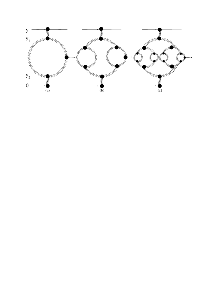
Figure 3: The special class of symmetric Pomeron loop diagrams taken into account in the sum over Pomeron loops.

In this letter, the special class of Pomeron loops shown in Fig. 3 have been taken into account in the summation over Pomeron loops. Diagrams of this type can be calculated from the observation that when each branch of the loop in Fig. 3 (a) gives birth to a loop, one obtains Fig. 3 (b). In this way a second generation of loops has been introduced, and Fig. 3 (b) is called the $N=2$ generation diagram. Fig. 3 (a) with one loop is called the $N=1$ generation diagram. Likewise, a third generation of loops has been introduced in Fig. 3 (c) when each of the 2 simple loops at the center of Fig. 3 (b) give birth to two loops in the same way, so Fig. 3 (c) is called the $N=3$ generation diagram. Continuing in this way, the full spectrum of symmetric Pomeron loop diagrams is generated for all $N$ generation diagrams. In this letter, an iterative algorithm is described for calculating such diagrams.

The solution to the BFKL equation provides the trajectory $\omega\left(n,\nu\right)$ $(n\in\mathbb{Z};\nu\in\mathbb{R})$ for the BFKL Pomeron as Fadin:1976 , Balitsky:1978 ;

$$\omega\left(n,\nu\right)=\bar{\alpha}_{s}\left(\psi\left(1\right)-\Re e\,\psi\left(\frac{1+n}{2}+i\nu\right)\right);\hskip 28.45274pt\bar{\alpha}_{s}\equiv\frac{\alpha_{s}N_{c}}{\pi}$$ (1)

$n$ represents the energy levels of the BFKL Pomeron, and $\nu$ is a continuous variable which one integrates over when calculating Feynman diagrams. The BFKL eigenfunction falls sharply with increasing $n$ and is only positive at high energy when $n=0$. Hence throughout this letter which is focussed on high energy scattering, $n=0$ is assumed and the argument $n$ is suppressed. Hence the BFKL Pomeron trajectory which is the sum over ladder diagrams of the type shown in Fig. 2 is described by the regge behavior $s^{\omega\left(\nu\right)}\equiv e^{\omega\left(\nu\right)y}$. The scattering amplitude of Fig. 2 is well known and has been calculated in refs. Miller:2006bi , Levin:2007wc , Miller:2009ca , Kozlov:2004sh , Navelet:2002zz , Navelet:1998yv , Navelet:1997xn ;

$$A_{(0)}\left(y,\delta y_{H}|\mbox{{Fig.~{}\ref{flrg1}}}\right)\!=\!\frac{\alpha_{s}^{2}}{4}A_{H}\!\int^{\infty}_{-\infty}\!\!\!d\nu h\left(\nu\right)\lambda\left(\nu\right)e^{\omega\left(\nu\right)\left(y-\delta y_{H}\right)}E_{\nu}E^{\prime}_{-\nu}$$ (2)

$$h\left(\nu\right)=\frac{2}{\pi^{4}}\nu^{2};\hskip 14.22636pt\lambda\left(\nu\right)=\frac{1}{16}\frac{1}{\left(1/4+\nu^{2}\right)^{2}};\hskip 14.22636ptE_{\nu}=\left(\frac{r_{12}}{r_{10}r_{20}}\right)^{1/2+i\nu}\left(\frac{r^{\ast}_{12}}{r^{\ast}_{10}r^{\ast}_{20}}\right)^{1/2-i\nu}$$ (3)

$h\left(\nu\right)$ is the integration measure which preserves conformal invariance Braun:2009sh , Braun:2005bv , $\lambda\left(\nu\right)$ is the Pomeron propagator in the conformal basis Braun:2009sh , Braun:2005bv and $E_{\nu}$ is the coupling of the BFKL Pomeron to the QCD color dipole Navelet:1997xn , Braun:2009sh , Braun:2005bv , in the dipole approach to proton proton scattering. Here $r_{12}=r_{1}-r_{2}$ is the transverse size of the dipole and $r_{10}=r_{1}-r_{0}$ where $r_{0}$ is the center of mass coordinate of the dipole. $\delta y_{H}=\ln\left(M_{H}^{2}/4s_{0}\right)\,\left(s_{0}=1\mbox{GeV}/\mbox{c}^{2}\right)$ is the rapidity gap occupied by the heavy Higgs boson, and $A_{H}=\left(N_{c}^{2}-1\right)\alpha_{s}2^{1/4}G_{F}^{1/2}/3\pi$; (where $G_{F}$ is the Fermi coupling) is the contribution to the scattering amplitude of the process Pomeron+Pomeron $\to$ Higgs derived in refs. Miller:2007pc , Ellis:1975ap , Ellis:1976yc , 2 , Rizzo:1979mf , Dawson:1990zj , 22 , which as shown in Fig. 2 proceeds mainly via the intermediate top quark triangle. The observation that the BFKL eigenfunction Eq. (1) has a saddle point $\nu=0$ means that one can expand the exponential in Eq. (2) as

$$\omega\left(\nu\right)=\omega\left(0\right)-\frac{1}{2}\nu^{2}\omega^{\prime\prime}\left(0\right)+\mathcal{O}\left(\nu^{2}\right);\hskip 14.22636pt\omega\left(0\right)=4\bar{\alpha}_{s}\ln 2;\hskip 14.22636pt\omega^{\prime\prime}\left(0\right)=28\bar{\alpha}_{s}\zeta\left(3\right)\,.$$ (4)

where $\zeta\left(3\right)=1.202$ is the Riemann zeta function. Using this expansion the integration in Eq. (2) is evaluated by the steepest descent method which yields the result Miller:2009ca ;

$$A_{(0)}\left(y,\delta y_{H}|\mbox{{Fig.~{}\ref{flrg1}}}\right)\! =\!\frac{\bar{\alpha}_{s}^{2}\left(2\pi\right)^{1/2}\,A_{H}}{2\pi^{2}N_{c}^{2}}\!\frac{e^{\omega\left(0\right)\left(y-\delta y_{H}\right)}}{\left(\omega^{\,\prime\prime}\left(0\right)\left(y-\delta y_{H}\right)\right)^{3/2}}$$ (5)

Eq. (5) is the bare scattering amplitude for the desired process of Fig. 2. The first order shadowing correction is the Pomeron loop shown in Fig. 3 (a). Using the same conventions, the scattering amplitude is given by the expression Miller:2009ca ;

$$A_{(1)}\left(y,\delta y_{H}|\mbox{{Fig.~{}\ref{fsopl}} (a)}\right)=\frac{\alpha_{s}^{2}}{4}A_{H}\!\int^{\infty}_{-\infty}\!\!\!d\nu h\left(\nu\right)\lambda^{2}\left(\nu\right)e^{\omega\left(\nu\right)\left(y-y_{12}\right)}d_{(1)}\left(\nu|y,\delta y_{H}\right)E_{\nu}E^{\prime}_{-\nu}$$ (6a)

$$d_{(1)}\left(\nu|y,\delta y_{H}\right)=\frac{1}{16}\int^{\infty}_{-\infty}\!\!\!d\nu_{1}h\left(\nu_{1}\right)\lambda\left(\nu_{1}\right)\int^{\infty}_{-\infty}\!\!\!d\nu_{2}h\left(\nu_{2}\right)\lambda\left(\nu_{2}\right)|\Gamma\left(\nu|\nu_{1},\nu_{2}\right)|^{2}$$ (6b)

$$\times\int^{y}_{\delta y_{H}}\!\!\!dy_{1}\!\int^{y-\delta y_{H}}_{0}\!\!\!\!\!\!dy_{2}e^{\left(\omega\left(\nu_{1}\right)+\omega\left(\nu_{2}\right)-\omega\left(\nu\right)\right)y_{12}-\omega\left(\nu_{1}\right)\delta y_{H}}$$

Figure 4: The triple Pomeron vertex, where lines indicate “reggiezed” gluons. (a) is the planar diagram, and (b) is the non planar diagram.

where $y_{12}=y_{1}-y_{2}$ is the rapidity gap which the loop fills (see Fig. 3 (a)). $|\Gamma\left(\nu|\nu_{1},\nu_{2}\right)|^{2}$ is the triple Pomeron vertex (TPV) for the splitting of a Pomeron with conformal variable $\nu$ into two Pomerons with conformal variables $\nu_{1}$ and $\nu_{2}$, shown in Fig. 4. The explicit expression is very complicated and its full form and the derivation can be found in refs. Korchemsky:1997fy , Bialas:1997ig . The TPV is the sum of the planar and non planar diagrams shown in Fig. 4 (a) and Fig. 4 (b), namely;

$$\Gamma\left(\nu,\nu_{1},\nu_{2}\right) =16\bar{\alpha}_{s}^{2}\left(\frac{1}{4}+\nu^{2}\right)^{2}\left(\underbrace{\Omega\left(\nu,\nu_{1},\nu_{2}\right)}+\frac{2\pi}{N_{c}^{2}}\underbrace{\Lambda\left(\nu,\nu_{1},\nu_{2}\right)\left(\chi\left(\nu\right)-\chi\left(\nu_{1}\right)-\chi\left(\nu_{2}\right)\right)}\right);$$

Fig. 4 (a)Fig. 4 (b)

$$\chi\left(\nu\right) =\Re e\left(\psi\left(1\right)-\psi\left(\frac{1}{2}+i\nu\right)\right)$$

In ref. Miller:2009ca it was shown that the two contributions to Eq. (6) stem from the regions I; $\left\{\nu,i\nu_{1},i\nu_{2}\right\}=\left\{0,1/2,1/2\right\}$ and region II; $\left\{i\nu,\nu_{1},\nu_{2}\right\}=\left\{1/2,0,0\right\}$, for which the TPV takes the following asymptotic form;

$$|\Gamma\left(\nu,i\nu_{1}=\frac{1}{2},i\nu_{2}=\frac{1}{2}\right)|^{2} =\frac{1}{2}\left(4\pi\right)^{6}\bar{\alpha}_{s}^{4}\left(1-\frac{1}{N_{c}^{2}}\right)^{2}\left(\frac{1}{4}+\nu^{2}\right)^{3}\chi\left(\nu\right)\frac{1-i\nu_{1}-i\nu_{2}}{\left(1/2-i\nu_{1}\right)^{2}\left(1/2-i\nu_{2}\right)^{2}}\hskip 14.22636pt$$ (8a)

$$|\Gamma\left(i\nu=\frac{1}{2},\nu_{1}=0,\nu_{2}=0\right)|^{2} =\frac{\left(4\pi\right)^{6}\bar{\alpha}_{s}^{4}}{N_{c}^{4}}\frac{1}{\left(1/4+\nu^{2}\right)}$$ (8b)

Eq. (8a) is dominated by the planar diagram which contains singularities in region I, and the non planar diagram which is non singular has been thrown away. Eq. (8b) is purely the contribution from the non planar diagram which contains singularities in region II, whereas the planar diagram is non singular in region II and is not included in Eq. (8b). Previous publications assumed that $N_{c}\to\infty$, so since the non planar diagram has a pre-factor of $1/N_{c}^{2}$, it was neglected. In this letter the non planar diagram has been taken into account and moreover it is the dominant contribution to the TPV for region II. The non planar TPV leads to the contribution to the loop amplitude of Fig. 3 (a) derived in Eq. (10b) below, which is the dominant contribution. Hence in this letter, the remarkable property of the Pomeron loop amplitude has been found, that the major contribution to the Pomeron loop amplitude stems from the non planar TPV.

Eq. (8a) and Eq. (8b) lead to two contributions to the Pomeron loop amplitude for regions I and II. For region I the $\nu_{1},\nu_{2}$ integrals in Eq. (6b) are evaluated by closing the contour on the upper half plane and summing over the residues at $i\nu_{1},i\nu_{2}=1/2$, and for region II the steepest descent method is used (see ref. Miller:2009ca where the details of this calculation are explained). The loop amplitude $d_{(1)}\left(\nu|y\right)$ is the sum of both contributions given in Eq. (9b) and Eq. (9c), namely Miller:2009ca ;

$$d_{(1)}\left(\nu|y,\delta y_{H}\right) =d\left(\frac{1}{4}+\nu^{2}\right)^{3}\chi\left(\nu\right)\,e^{-\omega\left(\nu\right)\delta y_{H}}\left(\omega\left(\nu\right)+\frac{1}{2}\omega^{2}\left(\nu\right)\left(y-\delta y_{H}\right)\right)$$ (9b)

$$+\frac{ae^{-\omega\left(0\right)\delta y_{H}}}{\left(1/4+\nu^{2}\right)}\int^{y}_{\delta y_{H}}\!\!\!dy_{1}\!\int^{y-\delta y_{H}}_{0}\!\!\!\!\!\!dy_{2}\frac{e^{\left(2\omega\left(0\right)-\omega\left(\nu\right)\right)y_{12}}}{y_{12}^{3/2}\left(y_{12}-\delta y_{H}\right)^{3/2}};$$

$$d =\bar{\alpha}_{s}\left(1-\frac{1}{N_{c}^{2}}\right)^{2};\hskip 14.22636pta=\frac{2^{10}\bar{\alpha}_{s}^{4}}{N_{c}^{4}\pi\left(\omega^{\prime\prime}\left(0\right)\right)^{3}}\,.$$ (9c)

Plugging Eq. (9) into Eq. (6a) leads to two contributions for the scattering amplitude of Fig. 3 (a). The first part stems from Eq. (9b) for region I, and the $\nu$ integral is evaluated by the method of steepest descents. The second piece stems from Eq. (9b) for region II, for which the $\nu$ integral is solved by closing the contour over the upper half plane and summing over the residues at $i\nu=1/2$, and afterwards integrating over the rapidity variables to yield finally the two expressions Miller:2009ca ;

$$A_{(1)}\left(y,\delta y_{H}|\mbox{{Fig.~{}\ref{fsopl}} (a)}\right) =\frac{\left(2\pi\right)^{1/2}\bar{\alpha}_{s}^{2}dA_{H}}{128\pi^{2}N_{c}^{2}}\frac{e^{\omega\left(0\right)\left(y-\delta y_{H}\right)}}{\left(\omega^{\prime\prime}\left(0\right)\left(y-\delta y_{H}\right)\right)^{3/2}}\chi\left(0\right)\left(\omega\left(0\right)+\frac{1}{2}\omega^{2}\left(0\right)\left(y-\delta y_{H}\right)\right)\hskip 14.22636pt$$ (10b)

$$+\frac{\bar{\alpha}_{s}aA_{H}}{2^{9}\pi N_{c}^{2}}\left(y-\delta y_{H}\right)\left(\frac{-1}{\bar{\alpha}_{s}}\frac{d}{dy}\right)^{3}\frac{e^{2\omega\left(0\right)\left(y-\delta y_{H}/2\right)}}{y^{3/2}\left(y-\delta y_{H}\right)^{3/2}}$$

Eq. (10b) is the part of the scattering amplitude which leads to the renormalization of the Pomeron intercept $\omega\left(0\right)$. Eq. (10b) is the dominant contribution, and is equivalent to 2 non interacting Pomerons, with renormalized Pomeron vertices. This can be seen from Fig. 3 (a), whereby at high energy taking out both branches of the loop, one is left with just two non interacting Pomeron exchanges. The same is true of the multiple loop diagrams of Fig. 3 (b) and (c), and all higher order symmetric loop diagrams, as will now be shown.

As explained above, Fig. 3 (b) stems from Fig. 3 (a) when each branch of the loop gives birth to a secondary loop leading to the two “second generation” of loops in Fig. 3 (b). In the same way when the second generation loops in Fig. 3 (b) each give birth to two loops, this leads to 4 “third generation” of loops in Fig. 3 (c). Continuing with this evolution, the entire spectrum of symmetric $N$ generation diagrams can be generated for all $N$ . The scattering amplitude with $N$ generations of loops shown in Fig. 5 is the generalization of Eq. (6a), namely Miller:2009ca ;

$$A_{(N)}\left(y,\delta y_{H}|\mbox{{Fig.~{}\ref{fpictN1}}}\right) =\frac{\alpha_{s}^{2}}{4}\int^{\infty}_{-\infty}\!\!\!d\nu h\left(\nu\right)\lambda^{2}\left(\nu\right)e^{\omega\left(\nu\right)y}d_{(N)}\left(\nu|y,\delta y_{H}\right)E_{\nu}E^{\prime}_{-\nu}A_{H}$$ (11)

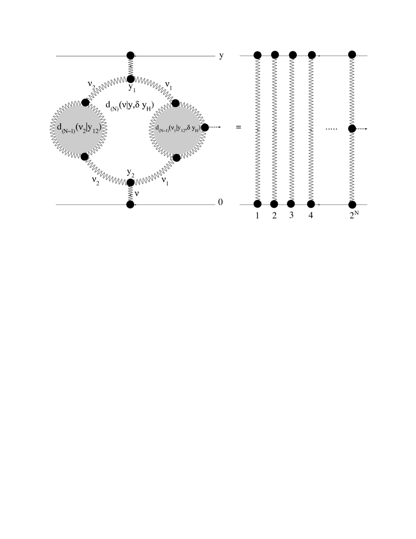
Figure 5: The $N$ generation diagram which stems from the simple loop giving birth to two sets of $N-1$ generations of loops, is equivalent to the diagram of $2^{N}$ non interacting Pomerons with renormalized Pomeron vertices.

where $d_{(N)}\left(\nu|y,\delta y_{H}\right)$ is the contribution of the $N$ generations of loops in Fig. 5. The way to calculate $d_{(N)}\left(\nu|y,\delta y_{H}\right)$ is based on the observation that Fig. 5 is equivalent to the simple loop diagram of Fig. 3 (a) when each branch in the loop gives birth to a set of $N-1$ generations of loops. This means that to write the expression for $d_{(N)}\left(\nu|y,\delta y_{H}\right)$, all that is needed is to modify the propagators for the branches of the loop in the expression of Eq. (6b) as;

$$\lambda\left(\nu_{1}\right)\to\lambda\left(\nu_{1}\right)d_{(N-1)}\left(\nu_{1}|y_{12},\delta y_{H}\right)\lambda\left(\nu_{1}\right);\hskip 14.22636pt\lambda\left(\nu_{2}\right)\to\lambda\left(\nu_{2}\right)d_{(N-1)}\left(\nu_{2}|y_{12}\right)\lambda\left(\nu_{2}\right)$$ (12)

where in the notation of Fig. 5, $d_{(N-1)}\left(\nu_{1}|y_{12},\delta y_{H}\right)$ labels the set of $N-1$ generations of loops on the right in Fig. 5 which includes the production of the Higgs, and $d_{(N-1)}\left(\nu_{2}|y_{12}\right)=d_{(N-1)}\left(\nu_{2}|y_{12},\delta y_{H}=0\right)$ labels the set of loops on the left in Fig. 5 where there is no Higgs production. After implementing Eq. (12) in Eq. (6b), one arrives at the following amplitude for the set of $N$ generations of loops Miller:2009ca ;

$$d_{(N)}\left(\nu|y,\delta y_{H}\right) =\frac{1}{16}\int^{\infty}_{-\infty}\!\!\!d\nu_{1}h\left(\nu_{1}\right)\lambda\left(\nu_{1}\right)\int^{\infty}_{-\infty}\!\!\!d\nu_{2}h\left(\nu_{2}\right)\lambda\left(\nu_{2}\right)|\Gamma\left(\nu|\nu_{1},\nu_{2}\right)|^{2}$$

$$\times\int^{y}_{\delta y_{H}}\!\!\!dy_{1}\!\int^{y-\delta y_{H}}_{0}\!\!\!\!\!\!dy_{2}e^{\left(\omega\left(\nu_{1}\right)+\omega\left(\nu_{2}\right)-\omega\left(\nu\right)\right)y_{12}-\omega\left(\nu_{1}\right)\delta y_{H}}d_{(N-1)}\left(\nu_{1}|y_{12},\delta y_{H}\right)d_{(N-1)}\left(\nu_{2}|y_{12}\right)$$

Eq. (Pomeron loop summation in perturbative QCD and the survival probability) forms an iterative expression. Using the technique of proof by induction, the following two formulae for the two contributions to Eq. (Pomeron loop summation in perturbative QCD and the survival probability) can be proved (see ref. Miller:2009ca ) which stem from the two asymptotic expressions for the TPV of Eq. (8a) and Eq. (8b);

$$d^{\,\footnotesize{\mbox{I}}}_{(N)}\left(\nu|y,\delta y_{H}\right)\,=\frac{\left(d\,d^{\,\prime}\right)^{2^{[N-1]}}\bar{\alpha}_{s}^{N-1}}{d^{\,\prime}}\left(\frac{1}{4}+\nu^{2}\right)^{3}\chi\left(\nu\right)\,e^{-\omega\left(\nu\right)\delta y_{H}}$$ (14a)

$$\hskip 73.97733pt\times\prod^{N}_{k=2}\bar{\alpha}_{s}^{\left(k-1\right)2^{[N-k]}}\left(\frac{k+1}{k}-\frac{\left(k+3\right)\left(k+2\right)\left(k+1\right)}{2k^{2}}\right)^{2^{[N-k]}-1}\,$$

$$\hskip 73.97733pt\times\prod^{N}_{k=2}\left(\frac{k+1}{k}-\frac{\left(k+3\right)\left(k+2\right)\left(k+1\right)}{2k^{2}}+\frac{k+1}{k}\delta y_{H}\right)\,$$

$$\hskip 73.97733pt\times\,\,\omega^{N-1}\left(\nu\right)\left(\omega\left(\nu\right)+\frac{\omega^{2}\left(\nu\right)\left(y_{1}-\delta y_{H}\right)}{N+1}\right)\hskip 142.26378pt\forall N\geq 1;$$

$$d^{\mbox{\footnotesize{II}}}_{(N)}\left(\nu|y,\delta y_{H}\right)=\frac{\left(ab\right)^{2^{[N-1]}}}{b}\left(\frac{1}{4}+\nu^{2}\right)^{3}\chi\left(\nu\right)e^{-\omega\left(\nu\right)\delta y_{H}}\int^{y}_{\delta y_{H}}\!\!\!\!\!dy_{1}\int^{y_{1}-\delta y_{H}}_{0}\!\!\!\!\!\!\!dy_{2}\,y_{12}^{2^{[N-1]}-N}\left(y_{12}-\delta y_{H}\right)^{N-1}\hskip 22.76228pt$$ (14b)

$$\hskip 73.97733pt\times\left\{\!\left(\frac{-1}{\bar{\alpha}_{s}}\frac{d}{dy_{12}}\right)^{3}\!\frac{e^{2\omega\left(0\right)\left(y_{12}-\delta y_{H}/2\right)}}{y_{12}^{3/2}\left(y_{12}-\delta y_{H}\right)^{3/2}}\!\right\}\!\left\{\!\left(\frac{-1}{\bar{\alpha}_{s}}\frac{d}{dy_{12}}\right)^{3}\!\frac{e^{2\omega\left(0\right)y_{12}}}{y_{12}^{3}}\!\right\}^{2^{[N-1]}-1}\hskip 14.22636pt\forall N\geq 1;$$

$$d=\bar{\alpha}_{s}\left(1-\frac{1}{N_{c}^{2}}\right)^{2};\hskip 14.22636ptd^{\,\prime}=\frac{\bar{\alpha}_{s}}{8}\left(1-\frac{1}{N_{c}^{2}}\right)^{2};\hskip 14.22636pta=\frac{2^{10}\bar{\alpha}_{s}^{4}}{N_{c}^{4}\pi[\omega^{\,\prime\prime}\left(0\right)]^{3}};\hskip 14.22636ptb=\frac{\bar{\alpha}_{s}^{2}}{2^{11}}\left(1-\frac{1}{N_{c}^{2}}\right)^{2}.$$ (14c)

Finally after inserting Eq. (14) into Eq. (11), one finds the following scattering amplitude for the diagram of Fig. 5 with $N$ generations of loops Miller:2009ca ;

$$A^{\,\footnotesize{\mbox{I}}}_{(N)}\left(y,\delta y_{H}|\mbox{{Fig.~{}\ref{fpictN1}}}\right)\, =\frac{\left(2\pi\right)^{1/2}\bar{\alpha}_{s}^{2}A_{H}}{128\pi^{2}N_{c}^{2}}\frac{\left(d\,d^{\,\prime}\right)^{2^{[N-1]}}}{d^{\,\prime}}\bar{\alpha}_{s}^{N-1}\chi\left(0\right)\frac{e^{\omega\left(0\right)\left(y-\delta y_{H}\right)}}{\left(\omega\left(0\right)^{\prime\prime}\left(y-\delta y_{H}\right)\right)^{3/2}}$$

$$\times\prod^{N}_{k=2}\bar{\alpha}_{s}^{\left(k-1\right)2^{[N-k]}}\left(\frac{k+1}{k}-\frac{\left(k+3\right)\left(k+2\right)\left(k+1\right)}{2k^{2}}\right)^{2^{[N-k]}-1}\,$$

$$\times\prod^{N}_{k=2}\left(\frac{k+1}{k}-\frac{\left(k+3\right)\left(k+2\right)\left(k+1\right)}{2k^{2}}+\frac{k+1}{k}\delta y_{H}\right)\,$$

$$\times\,\,\omega^{N-1}\left(0\right)\left(\omega\left(0\right)+\frac{\omega^{2}\left(0\right)\left(y_{1}-\delta y_{H}\right)}{N+1}\right)\,\hskip 99.58464pt\forall N\geq 1;\hskip 14.22636pt$$

$$A^{\mbox{\footnotesize{II}}}_{(N)}\left(y,\delta y_{H}|\mbox{{Fig.~{}\ref{fpictN1}}}\right) =\frac{\bar{\alpha}_{s}\,A_{H}}{2^{9}N_{c}^{2}\pi}\frac{\left(ab\right)^{2^{[N-1]}}}{b}y^{2^{[N-1]}-N}\left(y-\delta y_{H}\right)^{N}$$

$$\times\left\{\left(\frac{-1}{\bar{\alpha}_{s}}\frac{d}{dy}\right)^{3}\frac{e^{2\omega\left(0\right)\left(y-\delta y_{H}/2\right)}}{y^{3/2}\left(y-\delta y_{H}\right)^{3/2}}\!\right\}\!\left\{\!\!\left(\frac{-1}{\bar{\alpha}_{s}}\frac{d}{dy}\right)^{3}\!\!\frac{e^{2\omega\left(0\right)y}}{y^{3}}\!\!\right\}^{2^{[N-1]}-1}\forall N\geq 1.\hskip 34.14322pt$$

Eq. (15) is the contribution which leads to the renormalization of the Pomeron intercept. Eq. (15) is the piece which is equivalent to $2^{N}$ non interacting Pomerons, with renormalized Pomeron vertices shown pictorially in Fig. 5. This follows from the observation that Eq. (15) can be recast in the form;

$$A^{\mbox{\footnotesize{II}}}_{(N)}\left(y,\delta y_{H}|\mbox{{Fig.~{}\ref{fpictN1}}}\right)\equiv\kappa_{\mbox{\tiny{\it(N)}}}\,e^{2^{N}\omega\left(0\right)y}$$ (16)

Comparison of the RHS of Eq. (16)with Eq. (5) which is proportional to $e^{\omega\left(0\right)y}$, shows that
$A^{\mbox{\footnotesize{II}}}_{(N)}\left(y,\delta y_{H}|\mbox{{Fig.~{}\ref{fpictN1}}}\right)$ is equivalent to the amplitude of $2^{N}$ non interacting Pomerons, with a pre-factor $\kappa_{\mbox{\tiny{\it(N)}}}$ which contains the set of renormalized Pomeron vertices. The complete scattering amplitude is the sum of Eq. (15) and Eq. (15).

	$A_{(N)}\left(y=19,\delta y_{H}=\ln\left(M_{H}^{2}/4s_{0}\right)\right)$
	$\alpha_{s}=0.12$                $\alpha_{s}=0.2$
$N=0$	$1.57\times 10^{-8}\,\,\,\,$$\hskip 28.45274pt\,\,2.17\times 10^{-7}$
$N=1$	$2.05\times 10^{-10}\,\,$$\hskip 28.45274pt\,\,2.15\times 10^{-7}$
$N=2$	$2.85\times 10^{-15}\,\,$$\hskip 28.45274pt\,\,1.39\times 10^{-7}$
$N=3$	$3.40\times 10^{-24}\,\,$$\hskip 28.45274pt\,\,1.28\times 10^{-7}$
$N=4$	$8.20\times 10^{-42}\,\,$$\hskip 28.45274pt\,\,2.31\times 10^{-8}$
$N=5$	$8.13\times 10^{-77}\,\,$$\hskip 28.45274pt\,\,5.11\times 10^{-9}$
$N=6$	$1.36\times 10^{-146}\,\,$$\hskip 28.45274pt4.26\times 10^{-10}$

Table 1: Scattering amplitudes Miller:2009ca for diffractive Higgs production from the multiple Pomeron loop diagram with $N$ generations of loops. The mass of the Higgs boson is assumed to be $M_{H}=100\,\mbox{GeV}$, and the rapidity gap $y$ between the scattering protons is taken to be $y=19$, based on proton proton collisions at the typical LHC energy $\sqrt{s}=14$ TeV.

Table 1 Miller:2009ca shows the results up to the $N=6$ generation diagram. $N=0$ refers to the basic amplitude of Fig. 2 without loops derived in Eq. (5). The values in the table show that for the range of energies relevant to the LHC, the scattering amplitude falls as the number of generations of loops introduced increases. However from $N=0$ to $N=4$, for $\alpha_{s}=0.2$ the scattering amplitudes are the same order of magnitude. This demonstrates the importance of taking into account the full set of Pomeron loops for the summation over Pomeron loop diagrams. The difference in values for different choices of $\alpha_{s}$ show that the scattering amplitude is very sensitive to the choice of intercept.

The survival probability is a quantitative measure of the shadowing corrections to the basic diagram of Fig. 2. This stems from additional parton showers which produce inelastic scattering that destroy the large rapidity gaps. The contribution of hard re-scattrering to the survival probability can be derived from summing over the additional parton showers that stem from the Pomeron loop diagrams which have been calculated above. In this way, the “enhanced survival probability” $\langle\mid S_{\mbox{\footnotesize{enh}}}^{2}\mid\rangle$ is calculated by subtracting from the basic diagram of Fig. 2, the first correction from the $N=1$ generation diagram of Fig. 3 (a), and subtracting from this the $N=2$ generation diagram of Fig. 3 (b) , and so on, and divide by the basic amplitude of Fig. 2 itself to yield the correctly normalized survival probability which leads to the formula Miller:2009ca ;

$$\langle\mid S_{\mbox{\footnotesize{enh}}}^{2}\mid\rangle=1-\sum^{\infty}_{N=1}\left(-1\right)^{N-1}\frac{A_{(N)}\left(y,\delta y_{H}|\mbox{{Eq.~{}(\ref{AN2})}+{Eq.~{}(\ref{AN3})}}\right)}{A_{(0)}\left(y,\delta y_{H}|\mbox{{Eq.~{}(\ref{A01})}}\right)}$$ (17)

.

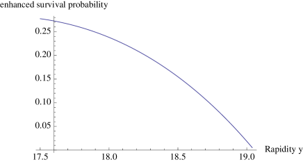
Figure 6: The enhanced survival probability $\langle\mid S_{\mbox{\footnotesize{enh}}}^{2}\mid\rangle$ plotted against the rapidity separation $y$ of the scattering protons. $\alpha_{s}=0.2$.

Fig. 6 Miller:2009ca is a plot of the energy dependence of the enhanced survival probability. The graph shows a decrease of the survival probability as the energy increases. For the LHC range of energies, the results show that the enhanced survival probability is small, and could even be less than 1%. Both of these observations are in agreement with the results found in refs. Miller:2006bi , Gotsman:2009vz , Gotsman:2009bn , Gotsman:2008tr . The decrease with energy is a natural consequence of the way the survival probability is defined. The survival probability measures the probability not to have extra parton showers other than the basic process of Fig. 2. Extra parton showers leading to unwanted inelastic scattering inevitably increase with the energy of the interaction, and this decreases the probability of exclusive Higgs production with large rapidity gaps in tact after the scattering.

In summary, the dominant contribution to the simple Pomeron loop of Fig. 3 (a) stems from the non planar triple Pomeron vertex shown in Fig. 4 (b), which has not been taken into account before. The formula for the multiple Pomeron loop diagram for $N$ generations of loops, has been derived in the perturbative QCD approach, whereas previous methods have relied on the mean field approximation. The multiple Pomeron loop amplitude has two contributions which lead to the renormalization of the Pomeron intercept, and the diagram of $2^{N}$ non interacting Pomerons for the $N$ generation diagram, with renormalized Pomeron vertices. Multiple Pomeron loop diagrams, other than the simple loop of Fig. 3 (a) contribute significantly to the summation over Pomeron loops, and need to be taken into account. Using this formula, the contribution of short distance interactions to the survival probability has been estimated, from the sum over Pomeron loop diagrams, in perturbative QCD. The survival probability decreases with energy, and for the LHC range of energies it is small and could even be less than 1%., in agreement with the findings of refs. Miller:2006bi , Gotsman:2009vz , Gotsman:2009bn , Gotsman:2008tr . The smallness of the enhanced survival probability show that short distance interactions contribute substantially.

We would like to thank E. Levin and G. Milhano for their careful reading and helpful advice in writing this paper. I would also like to thank L. Apolin$\acute{a}$rio, M. Braun, J. Dias De Deus, and G. Milhano for fruitful discussions on the subject. This research was supported by the Fundaç$\tilde{a}$o para ci$\acute{e}$ncia e a tecnologia (FCT), and CENTRA - Instituto Superior T$\acute{e}$cnico (IST), Lisbon.

References

• [1] L. B  Gribov, E. M. Levin, M. G. Ryskin, Phys. Rep. 100 (1983) 1
• [2] J. Bartels Nucl. Phys. B151 (1975) 293
• [3] L N. Lipatov in Perturbative quantum chromodynamics Ed. A. H. Mueller World Scientific, Singapore
• [4] H. Cheng, C. Y.  Lo Phys. Rev. D13 (1976) 1131
• [5] J.  Foreshaw, D.  Ross, Quantum Chromodynamics and the Pomeron. Cambridge University Press
• [6] I. Y. Pomeranchuk, Sov. Phys. 3 (1956) 306
• [7] L. B Okun, I. Y Pomeranchuk, Sov. Phys. JTEP 3 (1956) 307
• [8] V. S. Fadin,E. A. Kuraev,L. N. Lipatov, Sov.Phys. JTEP 44 (1976) 443
• [9] Y. Y. Balitsky, L. N. Lipatov, Sov J. Nucl. Phys. 28 (1978) 822
• [10] G. P. Korchemsky, Nucl. Phys.  B 550 (1999) 397 [arXiv:hep-ph/9711277].
• [11] A. Bialas, H. Navelet and R. B. Peschanski, Phys. Rev.  D 57 (1998) 6585 [arXiv:hep-ph/9711442].
• [12] J. S. Miller, Eur. Phys. J.  C 56 (2008) 39 [arXiv:hep-ph/0610427].
• [13] E. Levin, J. Miller and A. Prygarin, Nucl. Phys.  A 806 (2008) 245 [arXiv:0706.2944 [hep-ph]].
• [14] J. Miller, arXiv:0908.3450 [hep-ph].
• [15] M. Kozlov and E. Levin, Nucl. Phys.  A 739 (2004) 291 [arXiv:hep-ph/0401118].
• [16] H. Navelet and R. B. Peschanski, Nucl. Phys.  B 634 (2002) 291 [arXiv:hep-ph/0201285].
• [17] H. Navelet and R. B. Peschanski, Phys. Rev. Lett.  82 (1999) 1370 [arXiv:hep-ph/9809474].
• [18] H. Navelet and R. B. Peschanski, Nucl. Phys.  B 507 (1997) 353 [arXiv:hep-ph/9703238].
• [19] M. A. Braun, Eur. Phys. J.  C 63 (2009) 287 [arXiv:0901.3660 [hep-ph]].
• [20] M. A. Braun, arXiv:hep-ph/0504002.
• [21] J. S. Miller, arXiv:0704.1985 [hep-ph].
• [22] J. R. Ellis, M. K. Gaillard and D. V. Nanopoulos, Nucl. Phys.  B 106 (1976) 292.
• [23] J. R. Ellis, M. K. Gaillard and D. V. Nanopoulos,
• [24] J. Ellis et al., Nucl. Phys. B106 326- 331 (1976)
• [25] T. G. Rizzo, Phys. Rev.  D 22 (1980) 178 [Addendum-ibid.  D 22 (1980) 1824].
• [26] S. Dawson, Nucl. Phys.  B 359 (1991) 283.
• [27] S. Bentvelsen, E. Laenen, P. Motylinski, NIKHEF 2005 - 007
• [28] E. Gotsman, E. Levin, U. Maor and J. S. Miller, arXiv:0903.0247 [hep-ph].
• [29] E. Gotsman, E. Levin, U. Maor and J. S. Miller, arXiv:0901.1540 [hep-ph].
• [30] E. Gotsman, E. Levin, U. Maor and J. S. Miller, Eur. Phys. J.  C 57 (2008) 689 [arXiv:0805.2799 [hep-ph]].