Emergence of complex behaviour in gelling systems starting from simple behaviour of single clusters

Abstract

A theoretical and numerically study of dynamical properties in the sol-gel transition is presented. In particular, the complex phenomenology observed experimentally and numerically in gelling systems is reproduced in the framework of percolation theory, under simple assumptions on the relaxation of single clusters. By neglecting the correlation between particles belonging to different clusters, the quantities of interest (such as the self Intermediate Scattering Function, the dynamical susceptibility, the Van-Hove function, and the non-Gaussian parameter) are written as superposition of those due to single clusters. Connection between these behaviours and the critical exponents of percolation are given. The theoretical predictions are checked in a model for permanent gels, where bonds between monomers are described by a FENE potential. The data obtained in the numerical simulations are in good agreement with the analytical predictions.

I Introduction

The gelation transition transforms a viscous liquid (sol) into an elastic disordered solid (gel). In general this process is due to the formation of a macroscopic molecule, due to the bonding of multifunctional monomers in solution, which makes the system able to bear stress. The extent of the gelation process may be measured by the monomer volume fraction $\phi$, defined as $\phi=NV_{m}/V$, where $N$ is the number of monomers, $V_{m}$ is the single monomer volume and $V$ is the total system volume. On the static point of view, the sol-gel transition was interpreted flo ; deg in terms of the appearance of a percolating cluster of monomers linked by bonds stauffer , and experimental measurements of the geometric properties of gels have confirmed this correspondence (for a review see Stauffer et al.adconst and references therein).

Complex dynamical behaviours are observed in gelling systems already in the sol phase. For example, light scattering measurements show non-exponential decay of the intermediate scattering function, $F(k,t)$, in both permanent martin and thermoreversible physical gels ikkai ; ren . In particular power laws are observed at intermediate times, followed, at long times, by stretched exponential decays, $\exp(-(t/\tau)^{\beta})$, with $0<\beta<1$. In the gel phase, where ergodicity is broken, only the power law decay survives. Usually the onset of stretched exponential decays (present also in other complex systems, as spin glasses and glassy systems) is associated to the widening of relaxation times, which in gelling systems is due to the presence of a broad cluster size distribution close to the gelation threshold. However general predictions which connect this kind of relaxation to percolation theory are not easily feasible.

In this paper, assuming “simple” behaviours for the relaxation of clusters with given size, we show how the “complex” phenomenology of the relaxation in permanent gels may be obtained from the superposition of the behaviours of clusters with different sizes. In particular we are able to predict the behaviours of the self Intermediate Scattering Function, of the dynamical susceptibility, of the Van-Hove function, and of the non-Gaussian parameter, and to connect these behaviours to the cluster size distribution and the critical exponents of percolation. Then we check the theoretical predictions in a specific model for permanent gels, studied using Molecular Dynamics simulations.

The paper is organized as follows. In Sect.II the analytical results are briefly summarized, and in Sect.III they are compared with the data obtained by Molecular Dynamics simulations of a model for permanent gels, where bonds between monomers are described by a FENE potential FENEdum ; FENE ; tiziana_prl . In Sect.IV concluding remarks are discussed. Finally, in A, B and C the calculations are presented in details.

II Connection between static and dynamic properties

In this section we summarize our calculations, which will be show in details in appendices. We consider a system of randomly distributed monomers with a fixed volume fraction, $\phi$. At time $t=0$ permanent bonds are introduced at random between monomers at a distance $r<R$, where $R$ is suitably chosen. For a particular model see the FENE model FENEdum ; FENE ; tiziana_prl (Sect. IV), however the following arguments are independent on the details of the model.

Following the percolation approach flo ; deg , we identify the gel phase as the state where a percolating cluster is present. We denote by $\phi_{c}$ the volume fraction of the percolation threshold. In our calculations we use some results from percolation theory stauffer : In particular, in the sol phase, near the threshold, the cluster size distribution is given by $n(s)\propto s^{-\tau}e^{-s/s^{*}}$ (where $s^{*}$ is a cut-off value given by $\xi^{D_{f}}$, $D_{f}$ is the fractal dimension, and $\xi$ is the connectedness length which diverges at the threshold with the exponent $\nu$); in the gel phase, near the threshold, $sn(s)$ is put equal to $P_{\infty}\delta_{s,s_{max}}+Cs^{-\tau+1}e^{-(s/s^{*})^{(d-1)/d}}$, where $P_{\infty}$ is the density of particles in the percolating cluster of mass $s_{max}$, $d$ is the spatial dimension and $C$ is a constant. Moreover we assume that the relaxation time of clusters increases as a power law of the size theoryandexperimets , $\tau(s)\propto s^{x}$. With these assumptions, in the hypothesis of simple behaviour for single cluster (exponential relaxation, simple diffusion, etc.), we obtain all the complex phenomenology observed experimentally and numerically near the threshold in gelling systems. In particular we are able to predict the behaviours of the self Intermediate Scattering Function, of the dynamical susceptibility, of the Van-Hove function, and of the non-Gaussian parameter.

II.1 Self Intermediate Scattering Functions

We first consider the self Intermediate Scattering Functions (ISF):

$$F_{self}(k,t)=\left[\langle\Phi_{self}(k,t)\rangle\right]$$ (1)

where $\langle\dots\rangle$ is the thermal average over a fixed bond configuration, $\left[\dots\right]$ is the average over independent bond configurations of the system,

$$\Phi_{self}(k,t)=\frac{1}{N}\sum_{i=1}^{N}e^{i\vec{k}\cdot(\vec{r}_{i}(t)-\vec{r}_{i}(0))},$$ (2)

and $N$ is the number of particles. In the following we fix the wave vector $k=k_{min}$ and $k_{min}=2\pi/L$, with $L$ the linear system dimension.

In terms of the contributions due to different clusters, $F_{self}(k_{min},t)$ can be written as

$$F_{self}(k_{min},t)=\left[\sum_{s}sn(s)f_{s}(k_{min},t)\right],$$ (3)

where $n(s)$ is the cluster size distribution ($Nn(s)$ gives the number of clusters of size $s$) and $f_{s}(k,t)=\overline{\langle f_{C_{s}}(k,t)\rangle}$, where $f_{C_{s}}(k,t)=\frac{1}{s}\sum_{i\in C_{s}}e^{i\vec{k}\cdot(\vec{r}_{i}(t)-\vec{r}_{i}(0))}$ is the self ISF limited to a given cluster $C_{s}$ of size $s$, and $\overline{{{\dots}}}$ is the average over all clusters of given size $s$.

By replacing the sum with the integral, the self ISF for a given bond configuration becomes:

$$F_{self}(k_{min},t)\sim\int ds~{}sn(s)f_{s}(k_{min},t).$$ (4)

By assuming

$$f_{s}(k_{min},t)\simeq e^{-t/\tau(s)},$$ (5)

the integral in Eq.(4) gives in the thermodynamic limit the following predictions for the time dependence of $F_{self}(k_{min},t)$ in a permanent gel:

1. At the gelation threshold ($\phi=\phi_{c}$)

   $$F_{self}(k_{min},t)\propto~{}t^{-z}\Gamma(z),$$ (6)

   where $\Gamma(z)\equiv\int d\sigma~{}\sigma^{z-1}\exp(-\sigma)$ is the $\Gamma$-function with $z=(\tau-2)/x$.

2. In the sol phase ($\phi<\phi_{c}$)

   $$F_{self}(k_{min},t)\propto~{}t^{-c_{1}}e^{-(t/\tau_{\alpha})^{\beta}},$$ (7)

   where $\beta=1/(x+1)$, $c_{1}=\beta(\tau-3/2)$, and $\tau_{\alpha}\propto~{}(\phi_{c}-\phi)^{-f}$, and $f=xD_{f}\nu$. This approximated form, obtained in the long time limit, coincides with that suggested by Ogielskiogielski as fitting function for the time dependent order parameter in spin glasses, and it is in agreement with experimental martin and numerical cubetti findings in gelling systems.

3. In the gel phase ($\phi>\phi_{c}$)

   $$F_{self}(k_{min},t)\simeq P_{\infty}+At^{-c_{1}}e^{-(t/\tau_{\alpha})^{\beta}},$$ (8)

where $\beta=1/(x+1)$, and $c_{1}=\beta(\tau-3/2)$ are the same exponents obtained in the sol phase. The plateau value, $P_{\infty}$, gives the density of localized particles goldbart . Clearly the main contribution comes from localized particles of the percolating cluster, however a small contribution may be due to particles trapped inside it.

The calculations are shown in details in A.

Our findings given in Eq.s (6), (7) and Eq.(8) are in agreement with the theoretical predictions obtained in Ref.zippelius in the Rouse and Zimm models for randomly cross-linked monomers, where $x=1$ and $x=1/2$ respectively. Similar calculations are also done in Ref.sontolongo in a different context.

II.2 Fluctuations of the self ISF

In Ref. tiziana_prl it was studied the dynamical susceptibility, defined as the fluctuations of the self ISF:

$$\chi_{4}(k,t)=N\left[\rule{0.0pt}{10.0pt}\langle|\Phi_{self}(k,t)|^{2}\rangle-\langle\Phi_{self}(k,t)\rangle^{2}\right].$$ (9)

In particular it was shown that, in the sol phase, in the limit of $t\to\infty$ and $k\to 0$, $\chi_{4}(k,t)$ coincides with the mean cluster size, $S=\sum_{s}s^{2}n(s)$:

$$\lim_{k\to 0}\lim_{t\to\infty}\chi_{4}(k,t)=S,$$ (10)

which diverges at the threshold tiziana_prl with the exponent $\gamma$. Here we are interested in the time dependence of the dynamical susceptibility approaching the asymptotic value.

We neglect the contributions due to disconnected particles at each time $t$. In this way we can write $\chi_{4}(k,t)$ as a superposition of the contributions due to different clusters:

$$\chi_{4}(k,t)\simeq\left[\sum_{s}s^{2}n(s)\overline{\langle f_{C_{s}}(k,t)f^{*}_{C_{s}}(k,t)\rangle-\langle f_{C_{s}}(k,t)\rangle\langle f^{*}_{C_{s}}(k,t)\rangle}\right],$$ (11)

where again $f_{C_{s}}(k,t)=\frac{1}{s}\sum_{i\in C_{s}}e^{i\vec{k}\cdot(\vec{r}_{i}(t)-\vec{r}_{i}(0))}$ is the self ISF limited to a given cluster $C_{s}$ of size $s$, $\overline{{{\dots}}}$ is the average over all clusters of given size $s$, $\langle\dots\rangle$ is the thermal average over a fixed bond configuration, and $\left[\dots\right]$ is the average over independent bond configurations. The term $\langle f_{C_{s}}(k,t)f^{*}_{C_{s}}(k,t)\rangle$ in Eq.(11) can be written as

$$\langle f_{C_{s}}(k,t)f^{*}_{C_{s}}(k,t)\rangle =\frac{1}{s^{2}}\sum_{i,j\in C_{s}}\langle e^{i\vec{k}\cdot(\vec{r}_{i}(t)-\vec{r}_{j}(t))}e^{-i\vec{k}\cdot(\vec{r}_{i}(0)-\vec{r}_{j}(0))}\rangle$$ (12)

$$=\frac{1}{s^{2}}\sum_{i,j\in C_{s}}\langle e^{i\vec{k}\cdot\vec{\Delta}_{ij}(t)}\rangle,$$

where we have put $\vec{\Delta}_{ij}(t)\equiv(\vec{r}_{i}(t)-\vec{r}_{j}(t))-(\vec{r}_{i}(0)-\vec{r}_{j}(0))$. For connected particles $i$ and $j$, $|\vec{\Delta}_{ij}(t)|$ is finite, and in the low wave vector limit where $|\vec{\Delta}_{ij}(t)|\ll 1/k$ we can assume $e^{i\vec{k}\cdot\vec{\Delta}_{ij}(t)}\simeq 1$. Then, by supposing that $\overline{\langle f_{C_{s}}(k,t)\rangle\langle f^{*}_{C_{s}}(k,t)\rangle}=\overline{\langle f_{C_{s}}(k,t)\rangle}^{2}$, in the zero wave vector limit the dynamical susceptibility for a given bond configuration can be written as:

$$\lim_{k\to 0}\chi_{4}(k,t)\simeq\lim_{k\to 0}\sum_{s}s^{2}n(s)\left(1-\langle f_{s}(k,t)\rangle^{2}\right).$$ (13)

From this equation, using Eq.(5), it is direct to see that the dynamical susceptibility goes from zero (for $t=0$) to the mean cluster size $S$ (in the $t\to\infty$ limit), since the self ISF of clusters of given size, in the sol phase, goes from $1$ (for $t=0$) to zero (in the $t\to\infty$ limit).

As in the previous section we can evaluate $\lim_{k\to 0}\chi_{4}(k,t)$ in the sol phase, $\phi<\phi_{c}$. We find that, for time long enough, $\chi_{4}(k,t)$ approaches the asymptotic value in the following way:

$$\lim_{k\to 0}\chi_{4}(k,t)\simeq~{}S\cdot\left(1-At^{c_{2}}e^{-(2t/\tau_{\alpha})^{\beta}}\right),$$ (14)

where $\beta=1/(x+1)$ and $c_{2}=\beta(5/2-\tau)$. The exponent $\beta$ is exactly the same which appears in Eq.(7) for the decay to zero of the self ISF, the relaxation time in the stretched exponential function is given by $\tau_{\alpha}/2$, and finally the power law has a positive exponent $c_{2}$ different from the exponent $c_{1}$ which appears in Eq.(7).

The calculations are shown in details in B.

II.3 Self part of the Van-Hove function

The self part of the Van-Hove function hansen is given by:

$$G_{self}(r,t)=\frac{1}{N}\left[\langle\sum_{i=1}^{N}\delta(r-|{\bm{r}}_{i}(t)-{\bm{r}}_{i}(0)|)\rangle\right].$$ (15)

If the motion of particles is diffusive with a diffusion coefficient D, $G_{self}(r,t)=(1/4\pi Dt)^{3/2}\exp(-r^{2}/4Dt),$ where $r$ is the distance traveled by a particle in a time $t$. Deviations from the Gaussian distribution were observed in different glassy and gelling systems stariolo ; tiziana_pre . In fact the van-Hove function seems fitted by a Gaussian only for short distances, instead, for long distances, it is well fitted by an exponential tail that extends to larger distances for increasing times.

The deviation from the Gaussian distribution indicates that some particles move faster than others, due to the presence of heterogeneities. In permanent gels, heterogeneities coincide with clusters of particles connected by bonds tiziana_prl . As matter of fact particles belonging to different clusters have a different diffusion coefficient depending on the cluster size. As a consequence it has been suggested tiziana_pre that, in the sol phase and in the diffusive regime (i.e. in the long time limit), $G_{self}(r,t)$ is given by a superposition of Gaussians

$$G_{self}(r,t)=\left[\sum_{s}\frac{sn(s)}{(4\pi D(s)t)^{3/2}}\exp\left(-\frac{r^{2}}{4D(s)t}\right)\right],$$ (16)

where $D(s)$ is the diffusion coefficient of clusters of size $s$ and $n(s)$ is the cluster size distribution.

By assuming $\tau^{-1}(s)\propto D(s)=as^{-x}$, and by replacing the sum with the integral in Eq.(16), predictions can be given for the dependence of $G_{self}(r,t)$ on $r$ and $t$. We find, in the limit $r^{2}\gg at$:

$$t^{3/2}G_{self}(r,t)\propto\left(-A+\frac{1}{s^{*}}+\frac{xr^{2}}{4at}\right)^{-1}\exp\left[-\frac{r^{2}}{4at}\right],$$ (17)

where $A\equiv 1-\tau+3x/2$.

The calculations are shown in details in C.

II.4 Non-Gaussian parameter

The non-Gaussian parameter is defined as Rahman :

$$\alpha_{2}(t)=\left[\frac{3\langle\Delta r^{4}(t)\rangle}{5(\langle\Delta r^{2}(t)\rangle)^{2}}\right]-1,$$ (18)

where $\langle\Delta r^{2}(t)\rangle=\frac{1}{N}\sum_{i=1}^{N}\langle|\vec{r}_{i}(t)-\vec{r}_{i}(0)|^{2}\rangle$, and $\langle\Delta r^{4}(t)\rangle=\frac{1}{N}\sum_{i=1}^{N}\langle|\vec{r}_{i}(t)-\vec{r}_{i}(0)|^{4}\rangle$. It is easy to show Rahman that $\alpha_{2}(t)$ is zero if the probability distribution of the particle displacements is Gaussian.

Using Eq.(16), in permanent gels the non-Gaussian parameter is expected to tend in the long time limit to a plateau, whose value is given by

$$\alpha^{as}_{2}=\left[\frac{\sum_{s}sn(s)D^{2}(s)}{(\sum_{s}sn(s)D(s))^{2}}\right]-1=\left[\frac{\overline{D^{2}}-\overline{D}^{2}}{\overline{D}^{2}}\right],$$ (19)

where, for each bond configuration, $\overline{\dots}$ is the average over the cluster distribution. From this relation it appears clear that the deviation from gaussianity ($\alpha_{2}\neq 0$) is due to the fluctuations of the diffusion coefficient, which in turns is related to the presence of dynamical heterogeneities, i.e. groups of particles with different diffusion coefficient.

III FENE model for permanent gels

In this section we check the theoretical predictions obtained in Sect. II in the FENE model for permanent gels. We consider a $d=3$ system of $N$ particles interacting with a soft potential given by Weeks-Chandler-Andersen (WCA) potential chandler :

$$U_{ij}^{WCA}=\left\{\begin{array}[]{ll}4\epsilon[(\sigma/r_{ij})^{12}-(\sigma/r_{ij})^{6}+\frac{1}{4}],&r_{ij}<2^{1/6}\sigma\\ 0,&r_{ij}\geq 2^{1/6}\sigma\end{array}\right.$$ (20)

where $r_{ij}$ is the distance between the particles $i$ and $j$.

After the equilibration, at a given time $t=0$ particles distant less than $R_{0}$ are permanently linked by adding an attractive potential:

$$U_{ij}^{FENE}=\left\{\begin{array}[]{ll}-0.5k_{0}R_{0}^{2}\ln[1-(r_{ij}/R_{0})^{2}],&r_{ij}<R_{0}\\ \infty,&r_{ij}\geq R_{0}\end{array}\right.$$ (21)

representing a finitely extendable nonlinear elastic (FENE). The FENE potential was firstly introduced by WarnerFENEdum and is widely used to study linear polymers FENE . We choose $k_{0}=30\epsilon/\sigma^{2}$ and $R_{0}=1.5\sigma$ as usualFENE in order to avoid any bond crossing and to use an integration time step $\Delta t$ not too small.

We have performed Molecular Dynamics simulations of this model tiziana_prl : The equations of motion were solved in the canonical ensemble (with a Nosé-Hoover thermostat) using the velocity-Verlet algorithm Nose-Hoover with a time step $\Delta t=0.001\delta\tau$, where $\delta\tau=\sigma(m/\epsilon)^{1/2}$ is the standard unit time for a Lennard-Jones fluid and $m$ is the mass of particle. We use reduced units where the unit length is $\sigma$, the unit energy is $\epsilon$ and the Boltzmann constant $k_{B}$ is set equal to $1$. We choose periodic boundary conditions, and average all the investigated quantities over $32$ independent configurations of the system. The temperature is fixed at $T=2$ and the volume fraction $\phi=\pi\sigma^{3}N/6L^{3}$ (where $L$ is the linear size of the simulation box in units of $\sigma$) is varied from $\phi=0.06$ to $\phi=0.12$.

Using the percolation approach, we identify the gel phase as a state where a percolating cluster is present flo ; deg . With a finite size scaling analysis tiziana_prl we obtain that this transition is in the universality class of random percolation. In particular, we obtain that the cluster size distribution, $n(s)\sim s^{-\tau}$ at the gelation threshold $\phi_{c}=0.09\pm 0.01$, with $\tau=2.1\pm 0.2$; the mean cluster size $S(\phi)=\sum s^{2}n(s)\sim(\phi_{c}-\phi)^{-\gamma}$, with $\gamma=1.8\pm 0.1$; the connectedness length $\xi\sim(\phi_{c}-\phi)^{-\nu}$, with $\nu=0.88\pm 0.01$; and the fractal dimension of large clusters is $D_{f}=2.4\pm 0.1$. In the following we fix the number of particles, $N=1000$, where the threshold is $\phi_{c}\simeq 0.095$.

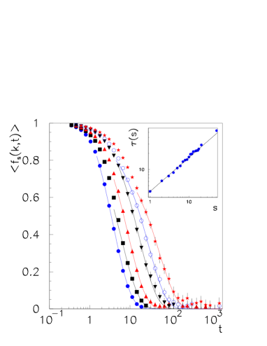
Figure 1: (Color online) Main frame: The self ISF, $\langle f_{s}(k,t)\rangle$ for clusters of size $s=1,2,4,10,21,52$, for $\phi=0.09$, $k=k_{min}$. The curves are exponential functions, $e^{-t/\tau(s)}$. Inset: The relaxation time, $\tau(s)$, as function of the cluster size $s$ for $k=k_{min}$ and $\phi=0.09$. The continuous curve is a power law $s^{x}$ with $x\simeq 0.65$.

III.1 Size dependence of dynamical behaviour of the clusters

In the sol phase we have studied the dynamical behaviour of the clusters as a function of the size $s$. In particular we have measured the self ISF and the mean squared displacement of clusters, respectively $\langle f_{s}(k,t)\rangle\equiv\frac{1}{s}\overline{\sum_{i\in C_{s}}\langle e^{i\vec{k}\cdot(\vec{r}_{i}(t)-\vec{r}_{i}(0))}\rangle}$, and $\langle\Delta r^{2}(s,t)\rangle\equiv\frac{1}{s}\overline{\sum_{i\in C_{s}}\langle|\vec{r}_{i}(t)-\vec{r}_{i}(0)|^{2}\rangle}$, where again $\overline{\dots}$ is the average of all clusters $C_{s}$ with fixed size $s$.

After an initial transient, we find that $\langle f_{s}(k,t)\rangle$ for $k=k_{min}$ is well fitted by exponential tail, $e^{-t/\tau(s)}$ (Fig.1), with $1/\tau(s)\propto s^{-x}$ (Inset of Fig.1) and $x$ not depending on the volume fraction. Our data furnishesnota_tau $x\sim 0.65$.

The mean squared displacement of clusters (shown in the main frame of Fig. 2), after a ballistic regime at short time, displays a diffusive behaviour. The diffusion coefficient of clusters, $D(s)$, obtained as $\langle\Delta r^{2}(s,t)\rangle\simeq 6D(s)t$, is plotted in the inset of Fig. 2 as a function of size $s$. In agreement with the results for the relaxation time, we find that $D(s)\propto s^{-x}$, with $x\simeq 0.67$.

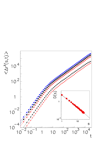
Figure 2: (Color online) Main frame: The mean squared displacement, $\langle\Delta r^{2}(s,t)\rangle$, for $\phi=0.09$, and clusters of size $s=1,2,4,10,21,52$. Inset: The diffusion coefficient, $D(s)$, as function of the cluster size $s$ for $\phi=0.09$. The continuous curve is a power law $s^{-x}$ with $x\sim 0.67$.

III.2 Self ISF and its fluctuations

In the sol phase, due to the superposition of the contributions of different clusters, the self ISF is expected to follow Eq.(7):

$$F_{self}(k_{min},t)\propto~{}t^{-c_{1}}e^{-(t/\tau_{\alpha})^{\beta}},$$ (22)

where $\beta=1/(x+1)\simeq 0.60$, $c_{1}=\beta(\tau-3/2)\simeq 0.36$, and $\tau_{\alpha}\propto~{}(\phi_{c}-\phi)^{-f}$, with $f=xD_{f}\nu\simeq 1.4$. $F_{self}(k_{min},t)$ is plotted in Fig. 3 for $\phi<\phi_{c}$. After the initial transient, the data are well fitted by the function, Eq.(7) (continuous curves in figures). Furthermore, in agreement with theoretical predictions, the relaxation time $\tau_{\alpha}$ (plotted in the Inset of Fig.3 as a function of $\phi$) appears to diverge approaching the transition threshold with the exponent $f\simeq 1.4$. At the threshold $\phi_{c}\simeq 0.095$ finite size effects appear.

Interestingly the presence of dynamical heterogeneities, i.e. groups of particles with different diffusion coefficient, is related to the breakdown of Stokes-Einstein relation. As shown in A, the relaxation time $\tau_{\alpha}$ is essentially the relaxation time of the critical cluster. On the contrary the diffusion coefficient of the system, obtained as $\langle\Delta r^{2}(t)\rangle\simeq 6Dt$, is given by the average over clusters with different sizes, $D\equiv\overline{D}=\sum_{s}sn(s)D(s)$. Since $D(s)\propto s^{-x}$, it is clear that $D$ is dominated by small clusters. As a consequence, although $\tau_{\alpha}$ diverges at the threshold, $D$ does not go to zero at $\phi_{c}$ (see Inset of Fig.3), due to the diffusion of small clusters through the gel matrix even for $\phi\gtrsim\phi_{c}$.

Figure 3: (Color online) Main Frame: Self ISF, $F_{self}(k,t)$ for $k=k_{min}$ and $\phi=0.06$, $0.07$, $0.08$, $0.085$, $0.09$, $0.095$ (from left to right) as a function of time $t$. The lines are fitting curves: $At^{-0.36}e^{-(t/\tau_{\alpha})^{0.6}}$. Inset: Structural relaxation time, $\tau_{\alpha}$ (full circles), compared with the inverse of the diffusion coefficient $20/D$ (full triangles) as a function of the volume fraction. The full line is the fitting curve: $\tau(\phi)\propto(\phi_{c}-\phi)^{-f}$, with $f\simeq 1.4$ and $\phi_{c}\simeq 0.095$.

Figure 4: (Color online) Self ISF, $F_{self}(k,t)$ for $k=k_{min}$ and $\phi=$ $0.1$,$0.105$,$0.11$,$0.12$.

Figure 5: (Color online) Dynamical susceptibility, $\chi_{4}(k_{min},t)$ for $\phi=0.06$, $0.07$, $0.08$, $0.085$ (from bottom to top) as a function of time $t$. The lines are fitting curves: $S\cdot\left(1-At^{0.24}e^{-(t/\tau^{\prime}_{\alpha})^{0.6}}\right)$.

In the gel phase a detailed analysis is not possible: $F_{self}(k_{min},t)$ (plotted in Fig.4 for $\phi>\phi_{c}$) displays a plateau, however at long times, due to finite size effects, it relaxes to zero following an exponential function.

Finally in the sol phase, we have also measured the dynamical susceptibility, $\chi_{4}(k,t)$, defined as the fluctuations of the self ISF, given by Eq.(9). In Fig.5, $\chi_{4}(k,t)$ is plotted for $k=k_{min}$ and different volume fractions. After the initial transient, the approach to the plateau is well fitted by Eq.(14):

$$\lim_{k\to 0}\chi_{4}(k,t)\simeq~{}S\cdot\left(1-At^{c_{2}}e^{-(t/\tau^{\prime}_{\alpha})^{\beta}}\right),$$ (23)

where $\beta=1/(x+1)\simeq 0.6$ and $c_{2}=\beta(5/2-\tau)\simeq 0.24$. Note that the relaxation time $\tau^{\prime}_{\alpha}$ coincides with $\tau_{\alpha}/2$ only at low volume fraction; near the threshold $\tau^{\prime}_{\alpha}$ is instead lower than $\tau_{\alpha}/2$, due to the contribution of disconnected particles at intermediate times.

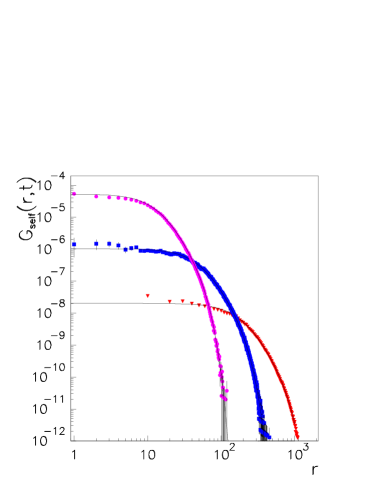
Figure 6: (Color online) The self part of the Van-Hove distribution for $\phi=0.07$ and time $t=~{}93.199,~{}1285.02,~{}17715.2$ (from top to bottom). Full lines are obtained from Eq.(16).

III.3 Self part of the Van-Hove function and the non-Gaussian parameter

In the sol phase we have also measured the self part of the Van-Hove function, $G_{self}(r,t)$, defined by Eq.(15). In the long time regime, $G_{self}(r,t)$ is fitted by a Gaussian curve only for short distances, and it seems well fitted by an exponential function for long distances tiziana_pre . In the long time regime, clusters of any size show a diffusive behaviour (see Fig. 2), then we have suggested tiziana_pre that $G_{self}(r,t)$ is given by a superposition of Gaussians, Eq.(16):

$$G_{self}(r,t)=\left[\sum_{s}\frac{sn(s)}{(4\pi D(s)t)^{3/2}}\exp\left(-\frac{r^{2}}{4D(s)t}\right)\right],$$ (24)

where $D(s)$ is the diffusion coefficient of clusters of size $s$, and $n(s)$ is the cluster size distribution. Data well agree with our hypothesis, as indicated in Fig.6, where we have used $n(s)$ and $D(s)$ measured in the simulations. As shown in the main frame of Fig. 7, $t^{3/2}G_{self}(r,t)$ plotted as a function of $r^{2}/t$ for fixed $\phi$ and for different times after the initial transient, collapse onto a single master curve, supporting the hypothesis that the data satisfy Eq.(24).

Finally the comparison with the approximate form obtained in C for $r^{2}\gg t$, Eq. (17),

$$t^{3/2}G_{self}(r,t)\propto\left(-A+\frac{1}{s^{*}}+\frac{xr^{2}}{4at}\right)^{-1}\exp\left[-\frac{r^{2}}{4at}\right],$$ (25)

(with $A\equiv 1-\tau+3x/2$, $s^{*}$ and $a$ obtained from the simulations) gives again a good agreement for high enough $r$ (Fig.7 and Inset). Note that the curves obtained from Eq.(25) and shown in figure are numerically indistinguishable from exponential functions in the considered range nota_exp (Inset of Fig.7).

In agreement with the above picture, we expect that the non-Gaussian parameter tends in the long time limit to a plateau, whose value coincides with the fluctuations of the diffusion coefficient, Eq.(19). In the main frame of Fig.8 the non-Gaussian parameter is plotted for different volume fractions, and in the inset of Fig.8 the plateau value is compared with the fluctuations of the diffusion coefficient. The data are in good agreement with Eq.(19), confirming that in permanent gels the non-gaussianity of the displacement distribution is due to the superposition of the contributions of clusters of different sizes. It is worth to notice that the main contribution to $\alpha_{2}(t)$ comes from small finite clusters. In fact, the bigger the cluster, the lower its diffusion coefficient and hence its contribution to the non-Gaussian parameter. Therefore, no criticality of the plateau value of the non-Gaussian parameter is observed approaching the transition threshold.

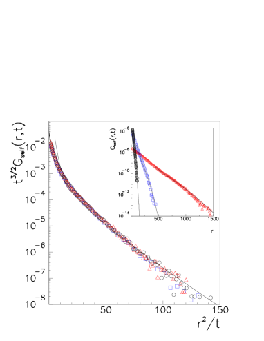
Figure 7: (Color online) Main frame: $t^{3/2}G_{self}(r,t)$ as a function of $r^{2}/t$ for $\phi=0.07$ and $t=~{}93.199,~{}1285.02,~{}17715.2$. The full line is obtained from Eq.(25). Inset: The self part of the Van-Hove distribution for $\phi=0.07$ and time $t=~{}93.199,~{}1285.02,~{}17715.2$ (from top to bottom). Full lines are obtained from Eq.(25) with the values of $s^{*}$, $x$, $\tau$ and $a$ measured in the simulations. Note that the curves shown in figure are numerically indistinguishable from exponential functions.

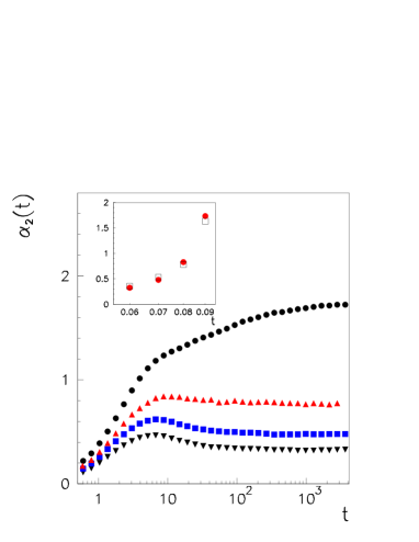
Figure 8: (Color online) Main frame: Non-Gaussian parameter, $\alpha_{2}(t)$, as a function of time $t$ for $\phi=~{}0.06$, $0.07$, $0.08$, $0.09$ (from bottom to top). Inset Asymptotic value of $\alpha_{2}(t)$ (empty squares) compared with the fluctuations of the diffusion coefficient given by Eq.(19) (full circles).

IV Conclusions

In this paper we show how the complex dynamics, such as stretched exponentials and power law behaviors, observed experimentally and numerically in gelling systems, emerges from the contribution of single clusters, which instead decay with a simple exponential. Furthermore, we establish a connection between this complex behaviour and critical exponents of percolation theory.

We also find, in the diffusive regime, an asymptotic form (for long enough distances) of the self part of the Van-Hove function, which deviates from the Gaussian distribution, and is numerically very similar to an exponential tail, usually observed in a large variety of complex system. Our finding suggest therefore that such deviation from Gaussianity may be due to a general mechanism, which may be ascribed to the presence of heterogeneities.

The theoretical predictions are found in agreement with numerical results, that we find in the FENE model for permanent gels. We suggest that a similar analysis can be extended to systems with finite lifetime bonds, as colloidal gels, glassy systems or spin glasses, where a “suitable” definition of clusters is necessary.

Appendix A Self Intermediate Scattering Functions

In this section we show in details the calculations which gives the predictions shown in Sect. III for the time dependence of the self ISF in the thermodynamic limit.

Starting from Eq.(4), in the hypothesis that $f_{s}(k_{min},t)\simeq e^{-t/\tau(s)}$, and $1/\tau(s)\sim as^{-x}$, the self ISF for a given bond configuration becomes:

$$F_{self}(k_{min},t)\simeq\int ds~{}sn(s)e^{-ats^{-x}}.$$ (26)

Let us consider three different cases: (i) $\phi=\phi_{c}$; (ii) $\phi<\phi_{c}$; (iii) $\phi>\phi_{c}$.

For $\phi\leq\phi_{c}$, $n(s)$ can be written as $n(s)\simeq s^{-\tau}\exp(-s/s^{*})$ stauffer , where $s^{*}$ is a cutoff value nota_k . Then we obtain:

$$F_{self}(k_{min},t)\simeq\int ds~{}\exp(t(s)),$$ (27)

where

$$t(s)\equiv-(\tau-1)\ln s-\frac{s}{s^{*}}-\frac{at}{s^{x}}.$$ (28)

(i) At the gelation threshold, $\phi=\phi_{c}$, $s^{*}\to\infty$, and the integral, Eq.(27), with $t(s)$ given by Eq.(28), can be evaluated exactly:

$$F_{self}(k_{min},t)\propto~{}t^{-z}\Gamma(z),$$ (29)

where $\Gamma(z)\equiv\int_{0}^{\infty}d\sigma~{}\sigma^{z-1}\exp(-\sigma)$ is the $\Gamma$-function with $z=(\tau-2)/x$.

(ii) In the sol phase, $\phi<\phi_{c}$, we are able to give only approximated predictions. The function $t(s)$, given by Eq.(28), has a maximum for $\tilde{s}$ such that nota_tilde

$$\frac{\tilde{s}}{s^{*}}=-(\tau-1)+\frac{xat}{\tilde{s}^{x}}.$$ (30)

Let us approximate $t(s)$ with $t(\tilde{s})-(s-\tilde{s})^{2}/(2\sigma^{2})$, where

$$\frac{1}{\sigma^{2}}\equiv-\left.\frac{d^{2}t(s)}{ds^{2}}\right|_{s=\tilde{s}}=\frac{1}{\tilde{s}^{2}}\left(-(\tau-1)+x(x+1)\frac{at}{\tilde{s}^{x}}\right).$$ (31)

If $\tilde{s}\gg\sigma$, $\int ds~{}\exp\left[-\frac{(s-\tilde{s})^{2}}{2\sigma^{2}}\right]=(2\pi\sigma^{2})^{1/2}$, and

$$F_{self}(k_{min},t)\simeq\exp\left[t(\tilde{s})\right]\int ds~{}\exp\left[-\frac{(s-\tilde{s})^{2}}{2\sigma^{2}}\right]$$

$$\propto\frac{1}{{\tilde{s}}^{(\tau-2)}}\left(-(\tau-1)+x(x+1)\frac{at}{\tilde{s}^{x}}\right)^{-1/2}\exp\left[-\left(\frac{\tilde{s}}{s^{*}}+\frac{at}{\tilde{s}^{x}}\right)\right].$$ (32)

Let us consider two limit cases: (1) $s^{*}\to\infty$; (2) $at/\tilde{s}^{x}\to\infty$.

(1) Using Eq.(30), Eq.(32) can be written in the following way:

$$F_{self}(k_{min},t)\propto\frac{\exp\left[-\frac{x+1}{x}\frac{\tilde{s}}{s^{*}}\right]}{{\tilde{s}}^{(\tau-2)}}\left(x(\tau-1)+(x+1)\frac{\tilde{s}}{s^{*}}\right)^{-1/2},$$ (33)

which in the limit $s^{*}\to\infty$, where $\tilde{s}\simeq\left(xat/(\tau-1)\right)^{1/x}$, gives again $F_{self}(k_{min},t)\propto~{}t^{-z}$ with $z=(\tau-2)/x$, in agreement with previous calculations.

(2) Using Eq.(30), Eq.(32) can be written in the following way:

$$F_{self}(k_{min},t)\propto\frac{\exp\left[-\frac{(x+1)at}{\tilde{s}^{x}}\right]}{{\tilde{s}}^{(\tau-2)}}\left(-(\tau-1)+x(x+1)\frac{at}{\tilde{s}^{x}}\right)^{-1/2}.$$ (34)

In the limit $at/\tilde{s}^{x}\to\infty$, $\tilde{s}\simeq(xas^{*}t)^{1/(x+1)}$, and we obtain

$$F_{self}(k_{min},t)\propto~{}t^{-c_{1}}e^{-(t/\tau_{\alpha})^{\beta}},$$ (35)

where $\beta=1/(x+1)$, $c_{1}=\beta(\tau-3/2)$, and $\tau_{\alpha}\propto~{}{s^{*}}^{x}$, which diverges at the threshold as power law with the exponent $f=xD_{f}\nu$.

(iii) Finally in the gel phase, $\phi>\phi_{c}$, $sn(s)$ in Eq.(26) can be written as nota_delta ; stauffer $sn(s)=P_{\infty}\delta_{s,s_{max}}+Cs^{-\tau+1}e^{-(s/s^{*})^{(d-1)/d}}$, where $P_{\infty}$ is fraction of particles belonging to the percolating cluster, $s_{max}$ is infinite in the thermodynamic limit, $d$ is the spatial dimension, and $C$ is a constant. Then, from Eq. (26), we obtain:

$$F_{self}(k_{min},t)\simeq P_{\infty}+C\int ds~{}\exp(t(s)),$$ (36)

where

$$t(s)\equiv-(\tau-1)\ln s-\left(\frac{s}{s^{*}}\right)^{(d-1)/d}-\frac{at}{s^{x}}.$$ (37)

Following the same arguments as in the sol phase, the second term in Eq. (36) is written as:

$$\int ds~{}\exp(t(s)) \propto \tilde{s}^{-(\tau-2)}\exp\left[-\left(1+\frac{xd}{d-1}\right)\left(\frac{at}{\tilde{s}^{x}}\right)\right]$$ (38)

$$\cdot \left(-\frac{(\tau-1)(d-1)}{d}+x\left(x+1-\frac{1}{d}\right)\frac{at}{\tilde{s}^{x}}\right)^{-1/2},$$

where the maximum point, $\tilde{s}$, of $t(s)$, Eq. (37), is obtained from

$$-(\tau-1)+\frac{axt}{\tilde{s}^{x}}=\frac{d-1}{d}\left(\frac{\tilde{s}}{s^{*}}\right)^{(d-1)/d}.$$ (39)

In the limit $at/\tilde{s}^{x}\to\infty$, $\tilde{s}\propto t^{1/(x+1-1/d)}$, and we obtain

$$F_{self}(k_{min},t)\simeq P_{\infty}+At^{-g}e^{-(t/\tau_{\alpha})^{\beta_{g}}},$$ (40)

where $\beta_{g}=(1-1/d)/(1-1/d+x)$, $g=\beta_{g}(\tau-3/2-1/2d)/(1-1/d)$.

For a finite system however $s_{max}$ is finite, and the behavior of $F_{self}(k_{min},t)$ is given by:

$$F_{self}(k_{min},t)\simeq\left\{\begin{array}[]{ll}P_{\infty}+At^{-g}e^{-(t/\tau_{\alpha})^{\beta_{g}}}&t\ll\tau_{max}\\ P_{\infty}~{}e^{-t/\tau_{max}}&t>\tau_{max},\end{array}\right.$$ (41)

where $\tau_{max}=\tau(s_{max})$ is the relaxation time of the percolating cluster.

Appendix B Fluctuations of the self ISF

In the hypothesis of the previous section (i.e. $\langle f_{s}(k,t)\rangle\simeq e^{-t/\tau(s)}$ and $1/\tau(s)\simeq as^{-x}$) Eq.(13) becomes

$$\lim_{k\to 0}\chi_{4}(k,t)=\sum_{s}s^{2}n(s)(1-e^{-2t/\tau(s)}),$$ (42)

which, for $\phi<\phi_{c}$, by replacing the sum with the integral, gives:

$$\lim_{k\to 0}\chi_{4}(k,t)\simeq S-\int ds\exp(w(s)),$$ (43)

where

$$w(s)\equiv-(\tau-2)\ln s-\frac{s}{s^{*}}-\frac{2at}{s^{x}}.$$ (44)

Note that the function $w(s)$ has a maximum for $\overline{s}$ such that

$$\frac{\overline{s}}{s^{*}}=-(\tau-2)+\frac{2xat}{\overline{s}^{x}}.$$ (45)

Let us approximate $w(s)$ with $w(\overline{s})-(s-\overline{s})^{2}/(2\sigma^{2})$, where

$$\frac{1}{\sigma^{2}}\equiv-\left.\frac{d^{2}w(s)}{ds^{2}}\right|_{s=\overline{s}}=\frac{1}{\overline{s}^{2}}\left((\tau-2)-x(x+1)\frac{2at}{\overline{s}^{x}}\right).$$ (46)

If $\overline{s}\gg\sigma$, $\int ds~{}\exp\left[-\frac{(s-\overline{s})^{2}}{2\sigma^{2}}\right]=(2\pi\sigma^{2})^{1/2}$, and

$$S-\lim_{k\to 0}\chi_{4}(k,t)\simeq\exp\left[w(\overline{s})\right]\int ds\exp\left(-\frac{(s-\overline{s})^{2}}{2\sigma^{2}}\right)$$

$$\propto\frac{1}{\overline{s}^{(\tau-3)}}\left((\tau-2)-x(x+1)\frac{2at}{\overline{s}^{x}}\right)^{-1/2}\exp\left[-\left(\frac{\overline{s}}{s^{*}}+\frac{2at}{\overline{s}^{x}}\right)\right].$$ (47)

The limit $at/\overline{s}^{x}\to\infty$, where $\overline{s}\propto(xs^{*}t)^{1/(x+1)}$, gives

$$\lim_{k\to 0}\chi_{4}(k,t)\simeq~{}S\cdot(1-At^{c_{2}}e^{-(2t/\tau_{\alpha})^{\beta}}),$$ (48)

where $\beta=1/(x+1)$ and $c_{2}=\beta(5/2-\tau)$. The exponent $\beta$ is exactly the same which appears in Eq.(7) for the decay to zero of the self ISF. Note that the relaxation time in the stretched exponential function is given by $\tau_{\alpha}/2$.

Appendix C Self part of the Van-Hove function

In the sol phase, where after an initial transient the system is found in a diffusive regime, we assume the validity of Eq.(16) for the self part of the Van-Hove function. By replacing the sum with the integral, and putting $D(s)\simeq as^{-x}$ , $G_{self}(r,t)$ can be written as

$$G_{self}(r,t)\simeq\frac{1}{(4\pi t)^{3/2}}\int ds~{}\exp\left(z(s)\right),$$ (49)

where

$$z(s)\equiv\left(1-\tau+\frac{3x}{2}\right)\ln s-\frac{s}{s^{*}}-\frac{s^{x}r^{2}}{4at}.$$ (50)

The condition for the first derivative of $z(s)$ to be zero gives:

$$\frac{s_{m}}{s^{*}}+\frac{xr^{2}s^{x}_{m}}{4at}=1-\tau+\frac{3}{2}x.$$ (51)

This equation admits a solution $s_{m}>0$ only if $A\equiv 1-\tau+3x/2>0$. Under this condition the solution of Eq.(51) is a maximum, in fact

$$-\left.\frac{d^{2}z(s)}{ds^{2}}\right|_{s=s_{m}} = \frac{1}{s_{m}^{2}}\left(A+x(x-1)\frac{r^{2}s^{x}_{m}}{4at}\right)>0,$$ (52)

is always true for $A>0$ (i.e. $x>2(\tau-1)/3$) notaA . In this case we can approximate $z(s)$ with $z(s_{m})-(s-s_{m})^{2}/(2\sigma^{2})$, where $\frac{1}{\sigma^{2}}\equiv-\left.\frac{d^{2}z(s)}{ds^{2}}\right|_{s=s_{m}}$. If $s_{m}\gg\sigma$, $\int ds~{}\exp\left[-\frac{(s-s_{m})^{2}}{2\sigma^{2}}\right]=(2\pi\sigma^{2})^{1/2},$ and we can write:

$$t^{3/2}G_{self}(r,t)\propto\exp\left[z(s_{m})\right]\int ds~{}\exp\left[-\frac{(s-s_{m})^{2}}{2\sigma^{2}}\right]$$

$$\propto s_{m}^{1+A}\exp\left[-\frac{s_{m}}{s^{*}}-\frac{r^{2}s^{x}_{m}}{4at}\right]\left(A+x(x-1)\frac{r^{2}s^{x}_{m}}{4at}\right)^{-1/2}.$$ (53)

Let us consider two limit cases: (i) $r^{2}\ll at$, and (ii) $r^{2}\gg at$. From Eq.(51) we obtain:

$$s_{m}\simeq\left\{\begin{array}[]{ll}As^{*}&r^{2}\ll at\\ \left(\frac{4Aat}{xr^{2}}\right)^{1/x}&r^{2}\gg at,\end{array}\right.$$ (54)

and Eq.(53) becomes:

$$t^{3/2}G_{self}(r,t)\propto\left\{\begin{array}[]{ll}\left(A+\frac{x(x-1)r^{2}}{4a^{\prime}t}\right)^{-1/2}\exp\left[-\frac{r^{2}}{4a^{\prime}t}\right]&r^{2}\ll at\\ \left(\frac{4Aat}{xr^{2}}\right)^{(A+1)/x}\exp\left[-\frac{A^{\prime}}{s^{*}}\left(\frac{4at}{r^{2}}\right)^{1/x}\right]&r^{2}\gg at,\end{array}\right.$$ (55)

where $a^{\prime}\equiv a/(As^{*})^{x}$, and $A^{\prime}=(A/x)^{(1/x)}$. Note that the condition $s_{m}\gg\sigma$ is satisfied in the limit $r^{2}/at\to 0$ where $s_{m}\to As^{*}$, which increases with increasing $x$ and/or approaching the gelation threshold. In the opposite limit, $r^{2}/at\to\infty$, $s_{m}\to 0$, and hence the condition $s_{m}\gg\sigma$ is not satisfied. In this case this approximation is expected not to hold and a development at the first order of the Taylor series of $z(s)$ around $s=1$ should be more appropriate (see below).

In the case $A\equiv 1-\tau+3x/2<0$ (as in the FENE model for permanent gels presented in Sect. III), $z(s)$ is a monotonic decreasing function of $s$:

$$\frac{dz}{ds}=\frac{A}{s}-\frac{1}{s^{*}}-\frac{xr^{2}s^{x-1}}{4at}<0.$$ (56)

Let us develop $z(s)$ at the first order of the Taylor series around the maximum $s_{m}=1$:

$$z(s)\simeq z(s_{m})+\left.\frac{dz}{ds}\right|_{s=s_{m}}(s-s_{m}).$$ (57)

By replacing Eq.(57) in Eq.(49), we obtain

$$t^{3/2}G_{self}(r,t)\propto\left(-\left.\frac{dz}{ds}\right|_{s=s_{m}}\right)^{-1}\exp\left[z(s_{m})\right]$$

$$\propto\left(-A+\frac{1}{s^{*}}+\frac{xr^{2}}{4at}\right)^{-1}\exp\left[-\frac{r^{2}}{4at}\right].$$ (58)

This approximation is expected to hold in the limit of long distances ($r^{2}\gg at$), where the second order of the Taylor series around $s_{m}=1$ is much smaller than the first one, and only a small interval of values of $s$ around $s_{m}=1$ contribute to the integral in Eq.(49).

The research is supported by CNR-INFM Parallel Computing Initiative, S.Co.P.E. and L.R. N.5 2005.

References

References

• (1) P. J. Flory, The Physics of Polymer Chemistry, Cornell University Press (1954).
• (2) P. G. de Gennes, Scaling Concepts in Polymer Physics, Cornell University Press (1993).
• (3) D. Stauffer, A. Aharony, Introduction to Percolation Theory, Taylor & Francis (1992).
• (4) D. Stauffer, A. Coniglio, M. Adam, Adv. poly. Sci. 44, 103 (1982).
• (5) J. E. Martin, J. Wilcoxon, D. Adolf Phys. Rev. A 36, 1803 (1987); J. E. Martin, J. P. Wilcoxon, Phys. Rev. Lett. 61, 373 (1988); J. E. Martin, J. P. Wilcoxon, J. Odinek, Phys. Rev. A 43, 858 (1991).
• (6) F. Ikkai, M. Shibayama Phys. Rev. Lett. 82, 4946 (1999).
• (7) S. Z. Ren, C. M. Sorensen Phys. Rev. Lett. 70, 1727 (1993).
• (8) H.R. Warner, Ind. Eng. Chem. Fundam. 11, 379 (1972)
• (9) K. Kremer, G. S. Grest, J. Chem. Phys. 92, 5057 (1990) and 94, 4103 (1991) (Erratum); G. S. Grest, K. Kremer Macromolecules 20, 1376 (1987); G. S. Grest, K. Kremer Phys. Rev. A 33, 3628 (1986); M. Murat, G. S. Grest Phys. Rev. Lett 63, 1074 (1989).
• (10) T. Abete, A. de Candia, E. Del Gado, A. Fierro, and A. Coniglio, Phys. Rev. Lett. 98, 088301 (2007).
• (11) M. Doi, S. F. Edwards, The Theory of Polymer Dynamics, Clarendon Press (1986).
• (12) As the relaxation time $\tau$ is dominated by the longest time $\tau(s^{*})$, we assume $\tau\simeq\tau(s^{*})\propto{s^{*}}^{x}$. Using that stauffer $s^{*}\propto\xi^{D_{f}}$, $\tau\simeq\xi^{2-\beta/\nu}$ and $2-\beta/\nu=D_{f}-1$, we obtain $x=(D_{f}-1)/D_{f}$, which in $d=3$ random percolation gives $x\simeq 0.6$.
• (13) A.T. Ogielski, Phys. Rev. B 32, 7384 (1985).
• (14) E. Del Gado, A. Fierro, L. de Arcangelis and A. Coniglio, Phys. Rev. E 69, 051103 (2004); E. Del Gado, L. de Arcangelis, and A. Coniglio, Eur. Phys. J. 2, 359 (2000).
• (15) W. Peng, H.E. Castillo, P.M. Goldbart, and A. Zippelius, Phys. Rev. B 57, 839 (1998); P.M. Goldbart, Proc. Conf. on Rigidity Theory and Applications (Traverse City, MI, 14-17 June 1998) ed M.F. Thorpe and P.M. Duxbury (New York: Kluwer/Plenum) pp 95-124; P.M. Goldbart, J. Phys.: Condens. Matter 12, 6585 (2000).
• (16) K. Broderix, P. M. Goldbart, and A. Zippelius, Phys. Rev. Lett. 79, 3688 (1997); M. Küntzel, H. Löwe, P. Müller and A. Zippelius, Eur. Phys. J. E 12, 325 (2003); H. Löwe, P. Müller and A. Zippelius, J. Phys.: Condens. Matter 17, S1659 (2005).
• (17) F. Brouers and O. Sontolongo-Costa, Europhys. Lett. 62, 808 (2003).
• (18) J.-P. Hansen and I. R. McDonald, Theory of Simple Liquids, 2nd ed. (Academic, London, 1986).
• (19) D. A. Stariolo, G. Fabricius, J. Chem. Phys. 125, 064505 (2006); P.I. Hurtado, L. Berthier, and W. Kob, Phys. Rev. Lett. 98, 135503 (2007); P. Chaudhuri, L. Berthier, and W. Kob, Phys. Rev. Lett. 99, 060604 (2007).
• (20) T. Abete, A. de Candia, E. Del Gado, A. Fierro, and A. Coniglio, Phys. Rev. E 78, 041404 (2008).
• (21) A. Rahman, Phys. Rev. 136, A405 (1964).
• (22) J.D. Weeks, D. Chandler, and H.C. Andersen, J. Chem. Phys 54, 5237 (1971).
• (23) S. Nosé, J. Chem. Phys 81, 511 (1984); W. G. Hoover, Phys. Rev. A 31, 1695 (1985); M. P. Allen, D. J. Tildesley Computer Simulation of Liquids Oxford Press (2000).
• (24) The function $g(r,t)=\ln[G_{self}(r,t)]$ can be approximated by a Taylor expansion around $r=r_{0}$. We observe that for $r\rightarrow\infty$, the second order term of the expansion of $g(r,t)$ is negligible respect the first order one, indicating that the curve in Eq.(25) resembles an exponential function of $r$ in the asymptotic regime. For finite $r$ it is always possible to find a range, whose amplitude depends on $r_{0}$ and $t$, in which the first order expansion represents a good approximation.
• (25) It is worth to notice that the cutoff value $s^{*}$ depends on the wave vector $k$. In fact $s^{*}=\xi^{D_{f}}f(k\xi)$, where $f(z)$ is a function which tends to a constant for small $z$, whereas it behaves as $z^{-D_{f}}$ for large values of $z$.
• (26) If $x=1$, the equation, Eq.(30), for $\tilde{s}$ becomes $\tilde{s}^{2}/s^{*}+(\tau-1)\tilde{s}-t=0$, which admits only one solution for $\tilde{s}>0$, $\tilde{s}=s^{*}\left(-(\tau-1)+\sqrt{(\tau-1)^{2}+4t/s^{*}}\right)/2$.
• (27) Actually we should consider $sn(s)=P_{\infty}g_{s,s_{max}}+Cs^{-\tau+1}e^{-(s/s^{*})^{(d-1)/d}}$, where $g_{s,s_{max}}$ is a distribution peaked around $s_{max}$, which tends to $\delta_{s,s_{max}}$ for $N\to\infty$ and $s_{max}\to\infty$.
• (28) By writing $\left.\frac{d^{2}z(s)}{ds^{2}}\right|_{s=s_{m}}$ in the following way: