Characteristic Velocities of Stripped-Envelope Core-Collapse Supernova Cores^∗

Abstract

The velocity of the inner ejecta of stripped-envelope core-collapse supernovae (CC-SNe) is studied by means of an analysis of their nebular spectra. Stripped-envelope CC-SNe are the result of the explosion of bare cores of massive stars ($\geq 8$ M_⊙), and their late-time spectra are typically dominated by a strong [O i] $\lambda\lambda$6300, 6363 emission line produced by the innermost, slow-moving ejecta which are not visible at earlier times as they are located below the photosphere. A characteristic velocity of the inner ejecta is obtained for a sample of 56 stripped-envelope CC-SNe of different spectral types (IIb, Ib, Ic) using direct measurements of the line width as well as spectral fitting. For most SNe, this value shows a small scatter around 4500 km s^-1. Observations ($<100$ days) of stripped-envelope CC-SNe have revealed a subclass of very energetic SNe, termed broad-lined SNe (BL-SNe) or hypernovae, which are characterised by broad absorption lines in the early-time spectra, indicative of outer ejecta moving at very high velocity ($v\geq 0.1c$). SNe identified as BL in the early phase show large variations of core velocities at late phases, with some having much higher and some having similar velocities with respect to regular CC-SNe. This might indicate asphericity of the inner ejecta of BL-SNe, a possibility we investigate using synthetic three-dimensional nebular spectra.

1 Introduction

Massive stars ($>8$ M_⊙) collapse when the nuclear fuel in their central regions is consumed, producing a core-collapse supernova (CC-SN) and forming a black hole or a neutron star. CC-SNe with a H-rich spectrum are classified as Type II. If the envelope was stripped to some degree prior to the explosion, the SNe are classified as Type IIb (strong He lines, and weak but clear H), Type Ib (strong He lines but no H), and Type Ic (no He or H lines) (Filippenko, 1997).

Some CC-SNe, called broad-lined SNe (BL-SNe), exhibit very broad absorption lines in their early phase, resulting from the presence of sufficiently massive ejecta expanding at high velocities. BL-SNe seem to be preferentially of Type Ic [two exceptions are the Type IIb SN 2003bg (Hamuy et al., 2009) and the Type Ib SN 2008D (Mazzali et al., 2008; Modjaz et al., 2009)]; see also SN 1987K (Filippenko, 1988), which is mentioned by (Hamuy et al., 2009). Some BL-SNe can reach kinetic energies of $\geq$ 10⁵² ergs. They are sometimes called hypernovae, and can be associated with long-duration gamma-ray bursts (GRBs) (see Woosley & Bloom, 2006, and references therein). However not all BL-SNe are associated with GRBs.

An important question in the context of CC-SNe is how the gravitational energy is converted into outward motion of the ejecta during the collapse; see (Janka et al., 2007) for a recent review. In GRB scenarios a relativistic outflow is launched by the central engine and deposits some fraction of its energy into the SN ejecta, probably preferentially along the polar axis, which might cause strong asymmetries (e.g., Maeda et al., 2002). The nearest, best-studied GRB-SNe are SN 1998bw / GRB 980425 (Galama et al., 1999), SN 2003dh / GRB 030329 (Matheson, 2004), SN 2003lw / GRB 031203 (Malesani et al., 2004), and SN 2006aj / GRB/XRF 060218 (Pian et al., 2006), although it is not fully established that the GRBs (or X-ray flashes) accompanying nearby CC-SNe can be compared directly to high-redshift GRBs. CC-SNe may be characterised by asphericities although a jet does not necessarily form (Blondin et al., 2003; Burrows et al., 2007; Kotake et al., 2004; Moiseenko et al., 2006; Takiwaki et al., 2009).

Extremely massive stars ($>100$ M_⊙) are thought to end their lives as pair-instability SNe (PI SNe). A star with enough mass to form a He core with more than 40 M_⊙ will suffer electron-positron pair instability, leading to rapid collapse. This triggers explosive oxygen burning, leading to the complete disruption of the star (Barkat et al., 1967; Heger & Woosley, 2005). This process can produce large amounts of ⁵⁶Ni. The ejecta mass and the explosion kinetic energy are high, but the ejecta velocities are moderate (Scannapieco et al., 2005).

Stripped CC-SNe, which lost part of their envelope before collapse, offer a clearer view of their inner ejecta than SNe which have retained it. Thus, in this paper we exclusively address stripped CC-SNe (Types IIb, Ib, Ic); we do not include Type II SNe, despite using the term “CC-SN.”

Asphericities in their inner and outer ejecta (e.g., Mazzali et al., 2001) are evident in at least some CC-SNe. Two main indicators are velocity differences of Fe and lighter-element lines, and polarisation measurements (e.g., Hoflich, 1991).

Independent of their type, with time SNe become increasingly transparent to optical light, as the ejecta thin out. At late times ($>200$ days after the explosion), the innermost layers of the SN can be observed. This epoch is called the nebular phase, because the spectrum turns from being absorption dominated to emission, mostly in forbidden lines. In this phase the radiated energy of a SN is provided by the decay of radioactive ⁵⁶Co (which is produced by the earlier decay of ⁵⁶Ni). Decaying ⁵⁶Co emits $\gamma$-rays and positrons which are absorbed by the SN ejecta. As the deposition rate of $\gamma$-rays and positrons depends on the density and ⁵⁶Ni distribution, the inner parts of the SN dominate the nebular spectra.

Recently, several authors (Maeda et al., 2008; Modjaz et al., 2008; Taubenberger et al., 2009) have studied nebular spectra of CC-SNe. They concentrated on the shape of the [O i] $\lambda\lambda$6300, 6364 doublet (which is produced by much of the mass) and concluded that torus-shaped oxygen distributions might cause the double-peaked [O i] profile observed in many CC-SNe nebular spectra. However, there is ongoing discussion regarding whether geometry is the dominant reason for this type of line profile (Milisavljevic et al., 2009, also see Appendix A).

Several authors have modelled nebular-phase spectra of SNe to derive quantities such as the ⁵⁶Ni mass (e.g., Mazzali et al., 2004; Stritzinger et al., 2006; Sauer et al., 2006; Maeda et al., 2007a), ejecta velocities (e.g., Mazzali et al., 2007b), asphericities (e.g., Mazzali et al., 2005, 2007a; Maeda et al., 2008), and elemental abundances (e.g., Maeda et al., 2007a, b). The nebular phase is especially suitable for studying the core of SNe. If different explosion scenarios are involved for different types of CC-SNe, one might expect the largest, most revealing differences to be in the central region of the explosion. Therefore, in contrast to the standard classification of BL-SNe, which is based primarily on early-time spectroscopy and describes the velocity field of the outer SN layers, here we focus on the centre of the explosion. We have modelled the nebular spectra of over 50 SNe, the largest sample of CC-SNe so far, and obtained a statistically significant representation of their core velocities.

We describe our data set in Section 2 and the modelling procedure in Section 3. In Section 4 we test the reliability of the modelling approach. Results are discussed in Section 5.

2 Data Set

We collected nebular spectra of 56 CC-SNe. This sample includes all the spectra presented by Matheson et al. (2001), Modjaz et al. (2008), and Taubenberger et al. (2009) for which a spectral fit was possible. The most important criteria for selection were a reasonable signal-to-noise ratio and a spectral coverage of at least the region between 6000 and 6500 Å. Most spectra range from 4000 to 10000 Å, allowing modelling of the Fe-group, oxygen, calcium, and carbon lines. If we found evidence for an underlying continuum, we tried to remove it using a linear fit. When several nebular spectra were available for a given SN, we chose the one closest to 200 days, although the precise epoch has little influence as long as the spectrum is nebular, as shown in Section 4.

Unfortunately, most of our spectra are not properly flux-calibrated. If an estimate of the ⁵⁶Ni mass was available in the literature for SNe with uncalibrated spectra, we used these values (Table 1). For the remaining SNe with uncalibrated spectra we tried to estimate the ⁵⁶Ni mass from the light curve. We emphasise that the exact ⁵⁶Ni mass is not important for our study, as we show in Section 4.

SN	log($L_{\rm Bol}$)	$M_{\rm Ni}$ (M⊙)	$\beta$	$M_{\rm ej,tot}$ ($M_{\odot}$)	$E_{\rm kin,tot}$ (1051 ergs)	References ($L_{\rm peak}$, $M_{\rm Ni}$, $M_{\rm tot}\&E_{\rm tot}$)
1990I	42.4	0.11 $\pm$ 0.02	0.044	3.7 $\pm$ 0.7	1.1 $\pm$ 0.1	1,1,1
1993J	42.2	0.08 $\pm$ 0.02	0.050	$\sim$3	$\sim$1	2,2,13
1994I	42.2	0.065 $\pm$ 0.03	0.041	$\sim$0.9	$\sim$ 1.0	3,3,7
1997dq	42.2	0.15 $\pm$ 0.03	0.095	$\sim$8–10	10–20	5,5,5
1997ef	42.2	0.135 $\pm$ 0.025	0.085	$\sim$8–10	10–20	4,5,5
1998bw	42.8	0.49 $\pm$ 0.04	0.079	$\sim$14	$\sim$60	3,3,15
2002ap	42.1	0.073 $\pm$ 0.02	0.058	2.5–5	4–10	3,3,14
2003jd	42.8	0.36 $\pm$ 0.04	0.057	3 $\pm$ 0.5	7${}^{+3}_{-2}$	3,3,3
2004aw	42.4	0.21 $\pm$ 0.03	0.084	3.5–8.0	3.5–9.0	3,16,16
2006aj	42.7	0.20 $\pm$ 0.04	0.040	$\sim$2	$\sim$2	3,12,12
2007Y	42.1	0.06 $\pm$ 0.01	0.048	$\sim$0.5	$\sim$0.1	8,8,8
2007gr	42.2	0.08 $\pm$ 0.02	0.046	1.5–3	1.5–3	10,11
2007ru	42.9	0.4	0.045	$1.3^{+1.1}_{-0.8}$	$5^{+4.7}_{-3.0}$	9,9,9
2008D	42.2	0.09 $\pm$ 0.02	0.057	$\sim$7	$\sim$6	4,4,4
2008ax	42.3	0.08 $\pm$ 0.02	0.040	3–6	$\sim$1	6,6,6

Table 1: Peak luminosities, ⁵⁶Ni masses, the ratio $\beta$ $\equiv$ $M_{\rm Ni}$ (M_⊙)/$L_{\rm Bol,42}$, the total ejecta mass, and the total kinetic energy for 15 CC-SNe taken from the literature (see references). Typically $\beta\approx 0.06$ with a dispersion of roughly 70%. References: ¹Elmhamdi et al. (2004), ²Bartunov et al. (1994), ³Valenti et al. (2008a), ⁴Mazzali et al. (2008), ⁵Mazzali et al. (2004), ⁶Pastorello et al. (2008), ⁷Sauer et al. (2006), ⁸Stritzinger et al. (2009), ⁹Sahu et al. (2009), ¹⁰ Hunter, in prep., ¹¹Valenti et al. (2008b), ¹²Mazzali et al. (2006), ¹³Nomoto et al. (1993), ¹⁴Mazzali et al. (2002), ¹⁵Nakamura et al. (2000), ¹⁶Taubenberger et al. (2006).

For several SNe only one light-curve point exists (generally the detection magnitude in the $V$ or $B$ bands, or unfiltered). To obtain a (very crude) estimate of the ⁵⁶Ni mass from this single data point we employed the following procedure. For the SNe with known ⁵⁶Ni mass and bolometric peak luminosity, the ratio of bolometric peak luminosity (in units of 10⁴² ergs) to ⁵⁶Ni mass (in units of M_⊙) can be calculated. This ratio varies between 0.040 and 0.095, with a rather uniform distribution (see Table 1), which reflects the variety of light-curve widths of different SNe (e.g., SNe with broader light curves have more ⁵⁶Ni for the same peak luminosity). From the estimates of the ⁵⁶Ni mass and the peak luminosity of these SNe, we can derive a relation

$$M_{Ni}({\rm M}_{\odot})\approx 0.058^{+0.042}_{-0.025}\,L_{\rm peak,42}.$$ (1)

This estimate should be compared with a similar one obtained for SNe Ia by Stritzinger et al. (2006), who found $M_{\rm Ni}$ (M_⊙) $=0.050\,L_{\rm peak,42}$. The difference probably arises from the different densities and compositions of SNe Ia and CC-SNe.

To estimate the peak luminosity from the measured magnitude, we first tried to determine the bolometric luminosity at the time of detection. For some SNe an estimate for both the Milky Way and host-galaxy absorption is available in the literature. For most SNe, however, only the former is known (Schlegel et al., 1998). In this case we assume a host-galaxy absorption between 0 and 1.0 mag (unfiltered) and treat this range as an uncertainty affecting our estimate. If the Milky Way absorption is not known as well, we assume an uncertainty between 0 and 1.5 mag (unfiltered). Unfiltered magnitudes are treated as bolometric, $V$-band magnitudes are converted to bolometric magnitudes using $m_{\rm Bol}=m_{V}-0.3\pm 0.2$ , and $B$-band magnitudes are converted using $m_{\rm Bol}=m_{B}-0.8\pm 0.4$. For the distance moduli and the errors in the distance we took the values listed in NED for the SN host galaxies (Virgo+GA+Shapley). We then estimated the epoch of detection (which is close to maximum light for most of the SNe of our sample) and the uncertainty in this value from the references given in Table 2. Comparing to light curves of well-observed SNe we determined the value and uncertainty of the peak luminosity, including uncertainties related to absorption, conversion from filtered to bolometric luminosity, and the lack of a well-sampled light curve. Combining this estimate with Equation (1), we obtained ⁵⁶Ni masses for all 56 SNe of our sample. These are listed in Tables 1 and 2. The possible error of this method is very large, spanning roughly a factor of 20. This uncertainty estimate is very conservative; for most SNe the actual error should be much smaller. However, it is sufficient for our purposes (as we show in the Section 4).

SN	$m$	$A_{V}$ (mag)	$m-M$ (mag)	$\Delta d$	log($L_{\rm peak}$)	$M_{\rm Ni}$	References ($m$, $A_{V}$)
1983N	11.3V	0.51 $\pm$ 0.05	28.02 $\pm$ 0.3	0 $\pm 5$	42.45${}^{+0.31}_{-0.22}$	0.17${}^{+0.43}_{-0.11}$	31,31
1985F	12.1B	0.70	29.72	0 $\pm 4$	43.08${}^{+0.33}_{-0.25}$	0.73${}^{+1.91}_{-0.49}$	1,2
1987M	-	-	-	-	43.00${}^{+0.18}_{-0.18}$	0.60${}^{+0.42}_{-0.25}$	3
1990B	-	2.64/5.46	-	-	-	0.2	34
1990U	15.8V	1.6	32.64	0 $\pm$ 12	42.93${}^{+0.44}_{-0.20}$	0.51${}^{+1.91}_{-0.32}$	4,5
1990W	14.8V	0.55	31.43	0 $\pm$ 3	42.43${}^{+0.60}_{-0.14}$	0.16${}^{+0.93}_{-0.09}$	6,*
1990aa	17.0N $\pm 0.5$	0.175	34.13	7 $\pm 7$	42.50${}^{+0.80}_{-0.20}$	0.19${}^{+1.84}_{-0.12}$	32,*
1990aj	-	-	-	-	-	0.2	33
1991A	18.0N	1.3	33.54	1 $\pm$ 10	42.19${}^{+0.31}_{-0.11}$	0.094${}^{+0.233}_{-0.051}$	5,5
1991L	-	-	-	-	-	0.2	35
1991N	13.9N	0.097	31.29	5 $\pm$ 5	42.53${}^{+0.56}_{-0.06}$	0.20${}^{+1.06}_{-0.10}$	36,*
1995bb	-	-	-	-	-	0.2	37
1996D	18.2V	0.509	34.04	0 $\pm$ 7	42.10${}^{+0.68}_{0.14}$	0.07${}^{+0.53}_{-0.04}$	38,*
1996N	-	-	-	-	-	0.2	29
1996aq	14.7V	0.129	32.20	0 $\pm$ 4	42.61${}^{+0.62}_{-0.14}$	0.24${}^{+1.48}_{-0.14}$	${}^{7},^{*}$
1997B	16.5N	0.243	33.17	10 $\pm$ 3	42.40${}^{+0.52}_{-0.06}$	0.15${}^{+0.70}_{-0.07}$	39,*
1997X	13.5N	0.091	31.15	4 $\pm$ 4	42.61${}^{+0.54}_{-0.06}$	0.25${}^{+1.21}_{-0.12}$	40,*
2000ew	14.9N	0.147	30.16	14 $\pm$ 7	41.88${}^{+0.60}_{-0.06}$	0.05${}^{+0.26}_{-0.02}$	41,*
2001ig	-	-	-	-	-	0.13${}^{+0.02}_{-0.02}$	8
2003bg	15.0N	0.096	31.24	14 $\pm$ 7	42.25${}^{+0.60}_{-0.06}$	0.11${}^{0.61}_{-0.07}$	10,*
2003dh	-	-	-	-	-	0.4${}^{+0.15}_{-0.1}$	9
2004ao	14.9N	0.348	32.35	0 $\pm$ 4	42.56${}^{0.54}_{-0.06}$	0.22${}^{+1.06}_{-0.11}$	13,*
2004dk	17.6N	0.522	32.15	$-$10 $\pm$ 10	41.87${}^{+0.66}_{-0.06}$	0.044${}^{+0.298}_{-0.021}$	15,*
2004gk	13.3N	0.10	31.02 (Virgo)	0 $\pm$ 5	42.56${}^{+0.56}_{-0.06}$	0.22${}^{+1.13}_{-0.11}$	14,*
2004gq	15.5N	-	-	-4 $\pm$ 3	-	0.2	30
2004gt	14.9N	0.22 $\pm$ 0.03	31.84	$-$3 $\pm$ 5	42.36${}^{+0.17}_{-0.07}$	0.14${}^{+0.21}_{-0.07}$	11,12
2004gv	17.6N	0.110	34.50	0 $\pm$ 7	42.38${}^{+0.60}_{-0.06}$	0.14${}^{+0.83}_{-0.07}$	27,*
2005N	-	-	-	-	-	0.2	42
2005bf	-	-	-	-	-	0.05${}^{+0.03}_{-0.03}$	26
2005kl	14.6N	$>>$ 1	-	-	-	0.2	22,28
2006F	16.7N	0.629	33.70	7 $\pm$ 7	42.63${}^{+0.60}_{-0.06}$	0.26${}^{+1.47}_{-0.12}$	19,*
2006T	17.4N	0.246	32.68	$-$11 $\pm$ 2	42.07${}^{+0.58}_{-0.14}$	0.07${}^{+0.383}_{-0.04}$	16,*
2006gi	16.3N	0.080	33.18	3 $\pm$ 5	42.28${}^{+0.56}_{0.06}$	0.11${}^{+0.59}_{-0.06}$	17,*
2006ld	16.0N	0.057	33.74	9 $\pm$ 4	42.73${}^{+0.54}_{-0.06}$	0.33${}^{+1.60}_{-0.16}$	18,*
2007C	15.9N	0.140	32.15	2 $\pm$ 4	42.03${}^{+0.54}_{-0.06}$	0.065${}^{+0.317}_{-0.032}$	20,*
2007I	18.0N	0/1.5	34.75 $\pm$ 0.25	10 $\pm$ 6	42.33${}^{+0.82}_{-0.10}$	0.13${}^{+1.33}_{-0.07}$	21,*
2007bi	18.3N	0/1.5	38.8	0 $\pm 10$	43.64${}^{+0.86}_{-0.06}$	2.6${}^{+29.4}_{-1.3}$	23,*
2007ce	17.4N	0/1.5	36.37	5 $\pm$ 3	43.12${}^{+0.72}_{-0.12}$	0.80${}^{+6.33}_{-0.44}$	43,*
2007rz	16.9N	0.660	33.59	7 $\pm$ 7	42.52${}^{+0.60}_{0.06}$	0.20${}^{+1.14}_{-0.10}$	24,*
2007uy	16.9N	0.075	32.48	$-$7 $\pm$ 7	41.84${}^{+0.60}_{-0.20}$	0.041${}^{+0.239}_{-0.026}$	25,*
2008aq	-	-	-	-	-	0.2	44

Table 2: Observed magnitude ($V$-band, $B$-band, $N$ = unfiltered CCD), extinction (in the $V$ band), distance modulus, epoch, estimated peak luminosity, and ⁵⁶Ni mass for 41 CC-SNe, together with references for the magnitude and absorption. For SNe 1987M, 2001ig, 2003dh, and 2005bf, estimates for the ⁵⁶Ni mass or luminosity are available and referenced. The uncertainty on the epoch was taken from Modjaz et al. (2008) and Taubenberger et al. (2009), if available, or estimated from the detection report. SNe without estimate for absorption are referenced with “*.” For SNe 2007ce, 2007I, and 2007bi, we have no information about the host galaxy, so we assumed an absorption between 0 and 1.5 mag (unfiltered). SN 2004gk is a member of the Virgo cluster and we therefore took the Virgo distance modulus for this SN, as no reliable estimate for the distance of the host galaxy is available. References: ¹Tsvetkov (1986), ²Begelman & Sarazin (1986), ³Nomoto et al. (1990), ⁴Clocchiatti & Wheeler (1997), ⁵Gomez & Lopez (1994), ⁶Elias et al. (1990), ⁷Nakano et al. (1996), ⁸Silverman et al. (2009a), ⁹Deng et al. (2005), ¹⁰Wood-Vasey & Chassagne (2003), ¹¹Monard et al. (2004), ¹²Maund et al. (2005), ¹³Singer & Li (2004), ¹⁴Quimby et al. (2004), ¹⁵Graham & Li (2004), ¹⁶Monard (2006), ¹⁷Itagaki et al. (2006), ¹⁸Frieman (2006), ¹⁹Dimai & Villi (2006), ²⁰Puckett et al. (2007), ²¹Jin et al. (2007), ²²Dimai & Migliardi (2005), ²³Nugent (2007), ²⁴Parisky & Li (2007), ²⁵Blondin & Calkins (2008), ²⁶Maeda et al. (2007b), ²⁷Monard et al. (2004), ²⁸Taubenberger et al. (2005) but absorption highly uncertain, assume a ⁵⁶Ni mass of 0.2 M_⊙, ²⁹Williams et al. (1996) but no light-curve information, assume a ⁵⁶Ni mass of 0.2 M_⊙, ³⁰Pugh et al. (2004) bu no distance information available, assume a ⁵⁶Ni mass of 0.2 M_⊙, ³¹Clocchiatti et al. (1996), ³²Perlmutter et al. (1990), ³³McNaught et al. (1991) but no light-curve information available, assume a ⁵⁶Ni mass of 0.2 M_⊙, ³⁴Clocchiatti et al. (2001) but distance and reddening highly uncertain, assume a ⁵⁶Ni mass of 0.2 M_⊙, ³⁵Pollas & Maury (1991) but no light-curve information, assume a ⁵⁶Ni mass of 0.2 M_⊙, ³⁶Filippenko & Korth (1991), ³⁷Tokarz et al. (1995) but no light-curve information available, assume a ⁵⁶Ni mass of 0.2 M_⊙, ³⁸Drissen et al. (1996), ³⁹Gabrijelcic et al. (1997), ⁴⁰Nakano et al. (1997), ⁴¹Puckett et al. (2000), ⁴²Schmidt et al. (2005) but no light-curve information, assume a ⁵⁶Ni mass of 0.2 M_⊙, ⁴³Quimby et al. (2007), ⁴⁴Brown et al. (2008) but no light-curve information and no detailed epoch information, assume a ⁵⁶Ni mass of 0.2 M_⊙.

SN	Type	Epoch (days)	1D	$v_{\alpha}$ (km s-1)	$v_{50}$ (km s-1)	Ref.
1983N	Ib	226	Y	3797	2630	∗
1985F	Ib/c	280	Y	4920	2456	∗
1987M	Ic	141	Y	5486	3701	∗
1990B	Ic	140	N	5405	5091	∗
1990I	Ib	237	Y	4828	2899	∗
1990U	Ic	184	Y	3488	3021	∗
1990W	Ib/c	183	Y	4803	3425	∗
1990aa	Ic	141	?	4216	4368	∗
1990aj	Ib/c	150-250	?	5122	3034	∗
1991A	Ic	177	Y	5262	3636	∗
1991L	Ib/c	100-150	N	4140	3316	∗
1991N	Ic	274	Y	4278	3239	∗
1993J	IIb	205	Y	4029	3070	∗
1994I	Ic	147	Y	5057	3967	∗
1995bb	Ib/c	150-400	Y	5154	4410	∗
1996D	Ic	214	Y	5228	3624	∗
1996N	Ib	224	N	3736	3047	∗
1996aq	Ib	226	N	5846	3451	∗
1997B	Ic	262	Y	4801	3317	∗
1997X	Ic	103	Y	4680	3420	∗
1997dq	BL-Ic	217	Y	4594	3361	∗
1997ef	BL-Ic	287	Y	4681	2733	∗
1998bw	BL-Ic	201	Y	6340	3602	∗
2000ew	Ic	122	N	4184	3001	∗
2001ig	IIb	256	N	5027	3241	Silverman et al. (2009b)
2002ap	BL-Ic	185	Y	6219	3729	∗
2003bg	BL-IIb	279	N	4736	3205	Hamuy et. al. (in prep.)
2003dh	BL-Ic	229	?	4342	3085	Bersier et. al. (in prep.)
2003jd	BL-Ic	317	N	6850	5593	∗
2004ao	Ib	191	N	4555	3158	Modjaz et al. (2008)
2004aw	Ic	236	Y	5007	3234	∗
2004dk	?	333	Y	5465	4338	Modjaz et al. (2008)
2004gk	Ic	225	Y	4623	3171	Modjaz et al. (2008)
2004gq	Ib	297	Y	6697	3039	Modjaz et al. (2008)
2004gt	Ic	160	N	4513	3371	∗
2004gv	Ib/c	299	Y	4792	3158	Modjaz et al. (2008)
2005N	Ib/c	70-120	N	4001	3591	∗
2005bf	Ib	209	N	3864	3628	Modjaz et al. (2008)
2005kl	Ic	160	Y	5074	3365	Modjaz et al. (2008)
2006F	Ib	314	N	4491	2966	Mazzali
2006T	?	371	N	4202	4436	∗
2006aj	BL-Ic	204	Y	6540	5100	∗
2006gi	?	148	Y	4589	3180	∗
2006ld	Ib	280	N	4086	3182	∗
2007C	Ib	165	N	4787	3520	∗
2007I	BL-Ic	165	N	6085	3277	∗
2007Y	Ib	270	Y	4331	3025	Stritzinger et al. (2009)
2007bi	PI?	360	Y	5487	3756	Mazzali
2007ce	BL-Ic	310	Y	6172	4461	Matheson
2007gr	Ic	158	Y	4480	3228	Valenti et al. (2009)
2007ru	BL-Ic	200	Y	5811	3981	Sahu et al. (2009)
2007rz	Ic	292	?	4998	3785	Mazzali
2007uy	Ib	111	Y	6103	4563	Mazzali
2008D	BL-Ib	86	N	5847	4040	Mazzali
2008aq	IIb	$>$130	Y	4119	2885	Matheson
2008ax	IIb	246	N	4100	2821	Navasardyan et. al. (in prep.)

Table 3: SN type (classified by early-phase spectra), the epoch of our spectra (relative to maximum light), and the characteristic velocities $v_{\alpha}$ and $v_{50}$ both corrected by 5% per 100 days. The maximum errors of $v_{\alpha}$ and $v_{50}$ are estimated to be $\pm$ 14% and $\pm$10%, respectively. SNe marked with “Y” are fit by our 1D shell modelling quite well. For SNe marked with “N” the central parts of the line profiles are not reproduced well and therefore probably could be improved with multi-dimensional modelling ($v_{\alpha}$ would not change much, as $v_{\alpha}$ is dominated by the outer parts of the line profiles, where most of the kinetic energy is located). For SNe marked with “?” the spectra are too noisy to categorise as “Y” or “N.” In total we have 12 BL-SNe (2 of them are GRB hypernovae), 17 regular SNe Ic (27 with BL-Ic), 12 regular SNe Ib (13 with BL-Ib), 4 regular SNe IIb (5 with BL-IIb), 1 possible PI SN, and 10 SNe for which the classification is unclear (they are certainly of the CC-SN type). See Taubenberger et al. (2009) for spectra referenced by “*.”

3 Spectral Modelling

The spectra were modelled using the nebular code of Mazzali et al. (2001, 2007a) in the stratified version. A Monte Carlo routine is used to calculate the deposition of energy (which is carried by the $\gamma$-rays and positrons produced by the decay of ⁵⁶Ni and ⁵⁶Co) in each shell. The gas heating caused by this process is balanced by cooling via line emission. The excitation and ionisation state of the gas, together with the electron density and temperatures, are then iterated until the line emissivity in each shell balances the deposited energy. The emission rate in each line is calculated solving a non-LTE matrix of rates to obtain the level populations (Axelrod, 1980).

The general principle of such modelling is that different velocity shells are characterised by different element abundances and densities, which lead to different ratios of line fluxes in each shell. The total emissivity of a shell is controlled by the energy deposition, which depends on the density and the ⁵⁶Ni mass of the shell and the neighbouring ones. Therefore, each shell has a certain emissivity integrated over all wavelengths and a characteristic line profile caused by the Doppler shift. Each line in the emerging spectrum is the result of the superposition of single components from each shell, with different characteristic widths. A change of the emissivity of one line results in a variety of profile variations of other lines which have to be modelled iteratively until the complex shape of the full spectrum is reproduced. As a complicated structure must be found in order to produce a certain spectrum, the method is quite reliable in determining the velocity field of the ejecta.

We start modelling each spectrum using a CC-SN model used by Mazzali et al. (2002) for SN 2002ap. Such a model contains all of the information about density, mass, velocity, and element abundances. We correct the ⁵⁶Ni mass to the values listed in Tables 1 and 2, and we scale the synthetic spectrum to match the observed one.

A clear modelling of the Fe-group lines is impossible for most nebular spectra because these lines are generally weak and are therefore affected by noise and background. The oxygen line is therefore taken as a tracer for the ⁵⁶Ni distribution. This means that our ⁵⁶Ni zone extends out to the point where the oxygen line can no longer be separated clearly from the background. Hence, a narrow oxygen line results in a more central ⁵⁶Ni distribution in our models, but it is important to note that this assumption may not exactly reflect the situation in real SNe. This may cause some epoch-dependent error which we try to quantify by comparing the time dependence of line widths in our models and the observed line widths (see Section 4). Above the ⁵⁶Ni/O zone we set the density to zero, as this region cannot be probed with the nebular approach. We discuss this in more detail in Section 4.

Other elements, such as O, Ca, and C, are distributed over the velocity shells until the line profiles are matched. We pay special attention to fitting the O line, since oxygen is typically the most abundant element in stripped-envelope CC-SNe.

The modelling process yields the abundances, masses, and velocities which best reproduce the observed spectra (see Figures 1 and 2 for two examples). The mass and velocity distribution can then be integrated to obtain the total mass and kinetic energy of the model. The ratio of core kinetic energy (in units of 10⁵⁰ ergs) to core mass (in units of M_⊙) is termed $\alpha$ in this paper:

$$\alpha\equiv\frac{E_{\rm kin,50}}{M_{\rm ej}({\rm M}_{\odot})}.$$ (2)

This parameter is measured for all 56 CC-SNe of our sample and is converted to a characteristic velocity (see Table 3),

$$v_{\alpha}=\Big{(}\frac{2\alpha 10^{40}}{{\rm M}_{\odot}{\rm[g]}}\Big{)}^{1/2}{\rm[km~{}s^{-1}]}.$$ (3)

The largest uncertainty in the estimate of $\alpha$ is caused by the background. The kinetic energy is dominated by the outer parts of the oxygen line and these are superposed on background lines and noise, which are difficult to distinguish. To quantify the uncertainty that this causes, we tried different fits for several spectra (see Figure 1 and 2 for two examples). We found that, depending on the background assumed, variations of up to $\pm 15$% in $\alpha$ can occur, which translates into an uncertainty of $\sim 7$% in $v_{\alpha}$. An exact treatment of this problem is difficult, as background subtraction is arbitrary to some degree. Therefore, based on this uncertainty, we estimate an error of 7% in $v_{\alpha}$.

As we show in Section 4, the line width slowly evolves with time, causing $v_{\alpha}$ to decrease by roughly 5% every 100 days. To handle this problem, we corrected $v_{\alpha}$ by $(1+0.05(t{\rm(days)}-200)/100)$ and assume that this causes an additional error of $\pm 5$% in $v_{\alpha}$.

In addition to $v_{\alpha}$, we also measure the half width of the oxygen doublet [O i] $\lambda\lambda$6300, 6364 at half-maximum intensity (HWHM), $\Delta_{50}$, for all SNe of our sample. This can be directly converted to a velocity via the redshift

$$v_{50}=\frac{\Delta_{50}}{6300}c,$$ (4)

where $c$ is the speed of light and $\Delta_{50}$ is given in Å units. This is another characteristic velocity of the SN core ejecta, which can be compared to $v_{\alpha}$ (see Figure 3). There seems to be a linear trend between $v_{50}$ and $v_{\alpha}$, as expected; exceptions are mostly caused by specific features of some line profiles, as discussed in detail in Section 4.

Estimating $v_{50}$ has the advantage that it can be done easily and it does not require modelling. The disadvantage is that $v_{50}$ contains some small contribution of the [O i] $\lambda$6364 line which causes some error. Since the ratio of [O i] $\lambda$6300 to [O i] $\lambda$6364 is $\sim$3 in the nebular phase, this error is small; it depends on the exact shape of the individual lines, but it should be $<$20% in the worst case, as we found by superposing Gaussians. More importantly, it is influenced by the shape of the inner line profile (which in some SNe has a double- or even triple-peaked shape) much more than by $v_{\alpha}$. In addition, $v_{50}$ measures the velocity at one point (half height), while $v_{\alpha}$ is the result of an integration over the entire line profile and includes the nonlinear weighting of different emission regions. The background causes some uncertainty in the estimate of $v_{50}$. We measure $v_{50}$ for several SNe while varying our assumptions about the background, and estimate an uncertainty of $\sim$5%. Moreover, we apply the same time-dependent correction as for $v_{\alpha}$ and assume an additional error as for $v_{\alpha}$ ($\pm 5$%). Adding the possible errors due to background, ⁵⁶Ni mass estimate, and time evolution of the line width, we estimate a maximum error of $\pm 14$% for $v_{\alpha}$ and $\pm 10$% for $v_{50}$, which does not necessarily mean that $v_{50}$ gives a more correct estimate of the core velocity.

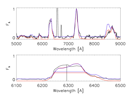
Figure 1: Nebular spectrum of SN 1990U ($v_{\alpha}=3450$(blue)/3633(red) km s^-1) at $t=184$ days (black) (upper panel) and the oxygen doublet [O i] $\lambda\lambda$6300, 6364 isolated (lower panel). Two models are shown in blue and red, illustrating the uncertainty in the background. This spectrum is the one with the lowest $v_{\alpha}$ in our sample (narrow oxygen line). The characteristic velocity is $v_{50}$ = 2996(blue)/3124(red) km s^-1. The horizontal lines show the full width at half-maximum intensity (FWHM).

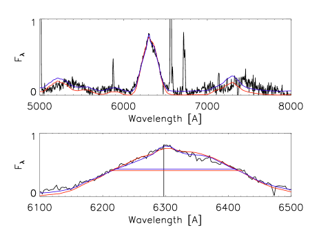
Figure 2: Nebular spectrum of the BL-SN 2006aj ($v_{\alpha}=6542$(blue)/6870(red) km s^-1) at $t=204$ days (black) (upper panel) and the oxygen doublet [O i] $\lambda\lambda$6300, 6364 isolated (lower panel). Two models are shown in blue and red, illustrating the uncertainty in the background. This spectrum has one of the highest $v_{\alpha}$ in our sample (broad oxygen line). The characteristic velocity $v_{50}$ = 4992(blue)/5190(red) km s^-1. The horizontal lines show the FWHM.

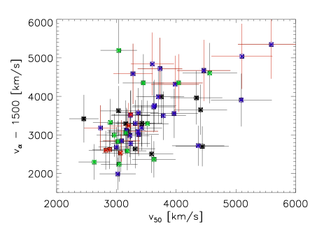
Figure 3: The characteristic velocities $v_{50}$ [km s^-1] vs. ($v_{\alpha}$ $-$ 1500 km s^-1). Both characteristic velocities seem to correlate (as expected). The offset by $\sim$1500 km s^-1 is caused by the different velocities cutoffs used to calculate $v_{50}$ (half height) and $v_{\alpha}$ (full line profile). BL-SNe are shown in red. SNe Ic are marked with blue, SNe Ib with green, and SNe IIb with red dots. Even taking into account the substantial errors, it is obvious that BL-SNe have a large scatter of characteristic core velocities. The data point at the upper right is SN 2003jd (see Table 3). The four BL-SNe at low characteristic velocities are SNe 1997ef, 1997dq, 2003dh, and 2003bg. The intermediate characteristic velocity BL-SNe are (from the left to the right) SNe 2007I, 1998bw, 2002ap, 2008D, 2007ce, and 2006aj. The three BL-SNe 2007I, 1998bw, and 2002ap fall off the $v_{\alpha}$/$v_{50}$ relation owing to the strong broadening toward the base of their [O i] $\lambda\lambda$6300, 6364 line.

4 Discussion

4.1 Tests

In order to ensure that the estimates of $v_{\alpha}$ are reliable, it is useful to verify that the data do not show behaviours that are not included in our modelling. Since the spectra that we used were obtained at very different SN epochs, it is vital that $v_{\alpha}$ does not depend strongly on SN epoch. Figure 4 shows the time evolution of $v_{\alpha}$ for three SNe with high-quality nebular spectra at several different epochs. The temporal evolution of $v_{\alpha}$ is in fact weak, at most $\sim$10% over 200 days, which is comparable to the general modelling uncertainty. Figure 5 shows the corresponding evolution of the line profiles. In Figure 6, $v_{\alpha}$ is plotted against SN epoch for the entire sample; no strong time dependence is seen. For $v_{50}$ the situation is similar. However, as can be seen for example in SN 1998bw (see Figures 4 and 5), small features in the line profile can have disturbing effects on $v_{50}$. The influence of epoch on the characteristic velocities will be more fully discussed in Section 4.2.

To test whether the often highly uncertain estimate of the ⁵⁶Ni mass influences $v_{\alpha}$, we alternatively increased and reduced the ⁵⁶Ni mass by a factor of five, therefore spanning a factor of 25 in ⁵⁶Ni mass for several randomly selected SNe of our sample. This corresponds roughly to the maximum uncertainty in the ⁵⁶Ni mass estimates. We found that $v_{\alpha}$ depends only weakly on ⁵⁶Ni mass: the difference is always less than 2%. For example, when changing the ⁵⁶Ni mass of SN 1987M by a factor of 25, from 0.6 to 0.024 $M_{\odot}$, $v_{\alpha}$ increased by only 1.3%, which is considerably smaller than other modelling uncertainties. Figure 7 shows $v_{\alpha}$ against ⁵⁶Ni mass; there is clearly no correlation. We conclude that the maximum error introduced by the uncertainty in the ⁵⁶Ni mass is $\pm 2\%$. The independence of $v_{\alpha}$ on ⁵⁶Ni mass is discussed in more detail in Section 4.2.

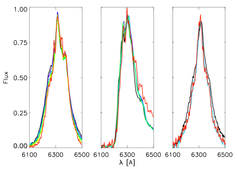
Figure 4: The [O i] $\lambda\lambda$6300, 6364 line profiles (left to right) of SN 2002ap (day 156, black; day 185, blue; day 237, violet; day 274, green; day 336, yellow; day 386, red), SN 1993J (day 205, black; day 236, blue; day 255, green; day 295, yellow; day 367, red), and SN 1998bw (day 201, black; day 337, red; day 376, blue). The temporal evolution is quantified in Figure 5.

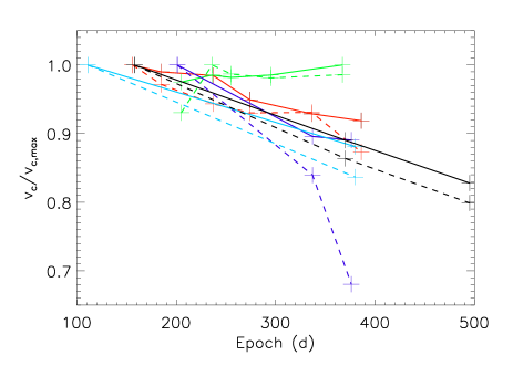
Figure 5: Temporal evolution of $v_{\alpha}$ (full line) and $v_{50}$ (dashed line) for SNe 2002ap (red), 1993J(green), 1998bw (blue), 2007uy (light blue), and 2007gr (black). One can see that variations are rather small, about 5% per 100 days. The rapid drop of $v_{50}$ of SN 1998bw is caused by the “knot” at half height of the oxygen-line profile, which “drops below” half height in the late phase. The increase of line width with time in SN 1993J must be some background effect (note the rise of the red wing at late times, due to H$\alpha$ emission) which could not be subtracted. For SNe 1993J, 1998bw, and 2002ap, similar temporal evolution was found by Taubenberger et al. (2009).

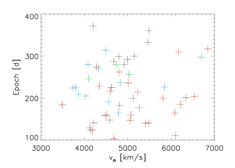
Figure 6: The epoch (days after maximum light) vs. characteristic velocity $v_{\alpha}$ (km s^-1) for all SNe at epochs listed in Table 3. SNe Ic are shown in red, SNe Ib in blue, and SNe IIb in green. SNe without type classification are shown in black. The effect of temporal line-width evolution is weak.

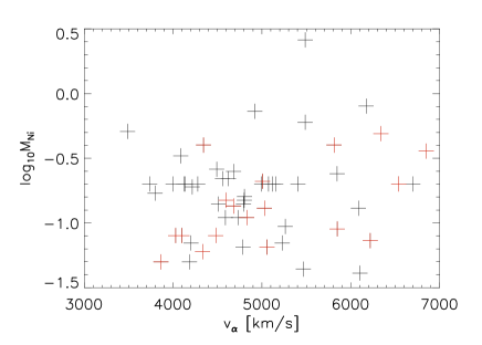
Figure 7: The logarithm of ⁵⁶Ni mass (in solar mass units) against the characteristic velocity $v_{\alpha}$. No relation is seen for our full sample. There might be a weak correlation for the SNe with ⁵⁶Ni mass estimates taken from the literature (shown in red), where the errors in the ⁵⁶Ni mass are much smaller. The mean ⁵⁶Ni mass of observed CC-SNe seems to lie around 0.20 M_⊙ (0.176 M_⊙ for ⁵⁶Ni mass estimates taken from the literature, 0.225 M_⊙ for the ⁵⁶Ni mass estimates in this paper), with a broad diversity. Neglecting the possible PI-SN 2007bi, ⁵⁶Ni masses range from 0.05 M_⊙ to 0.80 M_⊙. Because of the large uncertainties of our estimates, these upper and lower limits are inaccurate.

4.2 Discussion of the Method

We obtained characteristic velocities for 56 CC-SNe. Before we turn to the results we discuss our methodology.

In Section 2 we tried to determine the ⁵⁶Ni mass for 29 SNe in our sample without calibrated spectra. A typical uncertainty in ⁵⁶Ni mass is a factor of 5–10 up and a factor of 2–3 down. The uncertainty upward is mainly caused by the uncertainty in absorption and epoch. There are also uncertainties in distance, magnitude, converting magnitude to bolometric luminosity and finally to ⁵⁶Ni mass, which are smaller. Our ⁵⁶Ni masses might be systematically over- or underestimated and one should be cautious when using these values. The ⁵⁶Ni masses listed in the literature (18 SNe) have an average of 0.176 M_⊙, while the SNe with ⁵⁶Ni masses estimated in this paper have an average ⁵⁶Ni mass of 0.225 (28 SNe, excluding 9 SNe where we could not estimate a ⁵⁶Ni mass and excluding a possible PI-SN). Considering the relatively small numbers, the agreement is reasonable but might indicate a small systematic over-estimate of ⁵⁶Ni mass. In any case, as shown in Section 4.1, an uncertainty of a factor of 25 in ⁵⁶Ni mass will not influence our results significantly.

We checked for possible correlations between ⁵⁶Ni mass and $v_{\alpha}$. This could be important in two different ways. First, the uncertain estimate of the ⁵⁶Ni mass might introduce some error in the determination of $v_{\alpha}$. This is not the case, however, as shown in Section 4.1. Increasing the ⁵⁶Ni mass by a constant factor throughout the ejecta will increase the energy deposited in any shell by the same factor; hence, the relative contribution of each shell to the emission will remain constant. As the emitted energy per particle also remains rather constant (the mass of other elements must be increased accordingly to the ⁵⁶Ni mass), the spectrum of each shell does not change much. Therefore. the emerging spectrum is nearly constant apart from small differences arising from the small shift of line ratios in each shell (resulting, for example, from changes of the ionisation balance).

Second, there could be a physical correlation between ⁵⁶Ni mass and core ejecta velocities. For our full sample, this does not seem to be the case, as shown in Figure 7. However, our large uncertainties in the ⁵⁶Ni mass make a stringent conclusion impossible. There might be a weak correlation for the subgroup of 18 CC-SNe with ⁵⁶Ni masses taken from the literature (the uncertainties in these estimates should be much smaller), but the situation is not entirely clear owing to the substantial scatter.

Given that in most spectra we cannot determine the ⁵⁶Ni velocity very accurately (in CC-SN nebular spectra Fe-group lines are usually weak, strongly overlapping, and cannot be easily separated from the background), we can draw no conclusion about possible relations between ⁵⁶Ni mass and Fe-group element velocities, which might differ from light-element velocities in aspherical SN models. However, there is no correlation between the total kinetic energy or the total ejecta mass and the characteristic core velocity (for the 15 SNe listed in Table 1). A weak correlation of the ratio $(E_{\rm ej,tot}/M_{\rm ej,tot})^{1/2}$ with the characteristic core velocity is found, albeit with large scatter (see Figure 8).

The epoch at which a SN reaches its nebular phase generally depends on the mass and the ejecta velocity. Some of our spectra are quite early ($\sim$90 days after maximum light), though they all seem to be sufficiently nebular to be treated with our modelling. The epochs of our spectra vary between 100 and 400 days (after maximum light), and we have shown in Section 4 that this large span of epochs will not influence our results much. From detailed modelling of five SNe with good spectral coverage in the nebular phase (extending over 200 days), we can estimate that the characteristic velocity may decrease by $\sim$5% every 100 days. This is caused by the decreasing importance of the outer layers, which become less luminous.

In principle, if the behaviour of the positrons and the detailed distribution of ⁵⁶Ni were known, we could reproduce this line-width evolution. However, since these parameters are unknown, it is necessary to make some assumptions about both properties. As described in Section 3, we assumed that both the ⁵⁶Ni distribution and the positron deposition trace the oxygen line profile, leading to an oxygen line with constant width (since we assume local deposition of positron energy). This systematic error causes the discrepancy between the evolution of line width with epoch observed and our constant line width in the modelling, and it is taken into account in our treatment of temporal line-width evolution. Since this temporal evolution is weak, oxygen and ⁵⁶Ni cannot be strongly separated in the observed SNe and our modelling approach appears to resemble the physical situation quite well (e.g., a very central ⁵⁶Ni distribution would cause a rapid decrease of line width with time). Thus, we are convinced that our description of the ⁵⁶Ni core of the SNe is sufficiently accurate.

To enable a direct comparison to a parameter which can be obtained without any detailed modelling, we calculated the half width at half-maximum intensity of the oxygen doublet [O i] $\lambda\lambda$6300, 6364. These two lines are separated by $\sim$64 Å, which translates to a velocity of $\sim$3000 km s^-1. With decreasing density the intensity ratio of the two lines will shift from 1:1 to 1:3 (Li & McCray, 1992; Chugai, 1992), and in the nebular phase the ratio should lie somewhere between 1:2 and 1:3. The error in our characteristic velocity caused by the superposition of these two lines will therefore be small.

In Section 2 we already mentioned the advantages of both $v_{\alpha}$ and $v_{50}$. While $v_{\alpha}$ is time consuming to compute, $v_{50}$ is less exact in characterising the velocity of the central ejecta. In Figure 3 one can see a rather linear trend between both characteristic velocities, as expected. There are, however, some outliers. The SNe in the upper-left corner (where $v_{\alpha}-1500$ km s${}^{-1}>>v_{50}$) are SNe 1998bw, 2004gq, and 2007I. Both BL-SNe (SN 1998bw, 2007I) have very convex line profiles with a broad base and a sharp peak. SN 2004gq, the most extreme outlier, also has a convex shape; in addition, it shows a kink in the line profile, which explains the large difference between $v_{\alpha}$ and $v_{50}$ for this case. The SNe in the lower-right region (where $v_{\alpha}-1500$ km s${}^{-1}<<v_{50}$) are SNe 1990aa, 1990B, 2005bf, and 2006T. SN 1990aa has a prominent “spike” exactly at half height in the blue wing of the line profile, artificially increasing $v_{50}$ without affecting $v_{\alpha}$. SN 1990B has a very steep blue wing. SNe 2005bf and 2006T both have double-peaked [O i] profiles with a very steeply falling blue wing. The width at half height is almost the same as at the base of the line, which explains the low $v_{\alpha}/v_{50}$ ratio (see Figure 9 for the different line profiles). These examples demonstrate how $v_{50}$ can give a misleading picture of the characteristic core velocity in some cases. Hence, while in general $v_{50}$ seems to be a good proxy of core velocity, it should not be used if the [O i] profile shows broad double peaks, spikes, and kinks, or unusually steep or convex wings.

Both estimates of characteristic velocity are affected by the presence of an underlying continuum, which can either be the host galaxy or residual continuum emission form the SN. It is often difficult to distinguish the continuum from the SN spectrum. We tried to overcome this problem setting a characteristic minima around the oxygen line to zero flux by removing some linear function from the spectrum. However, the continuum in most cases is probably not represented by a linear function. Thus, some additional flux is almost always present in the region of an emission line, causing an error in the modelling procedure and in the determination of the half height. Consequently, it is not possible to obtain a single “best” result for a given spectrum. Depending on the quality and the specific shape of a spectrum, there might be a variety of possible background subtractions. To cope with this problem, we tried to model the extrema of what seemed plausible subtractions — of course a rather arbitrary approach. We modelled several different SNe in this manner to get a quantitative estimate of the typical uncertainty and found that an error of $\pm 7$% should cover the plausible range (e.g., see Figures 1 and 2, where the differences in characteristic velocity for the models shown are about 5%).

Another general uncertainty which we cannot quantify is introduced by possible global asphericities of the SN ejecta. In such a case the projected velocities might be considerably lower than the actual ejecta velocities, so the SN kinetic energy may be underestimated. As long as the ejecta geometry and inclination are unknown, this problem could not be removed by three-dimensional (3D) modelling either.

For 19 SNe ($\sim$35% of our sample), the shell modelling approach is not adequate to fit the central parts of the oxygen doublet. This suggests that at least 35% of the CC-SNe of our sample might be aspherical in the very centre (for other explanations, see e.g. Milisavljevic et al., 2009). Taubenberger et al. (2009) came to a similar conclusion. Of course, asphericities cannot be ruled out for the rest of our sample, even if the shell modelling approach was sufficient to obtain a good fit to the full line profile. As $v_{\alpha}$ is dominated by the outer parts of the line profile, a discrepancy between the model and the observation in the central parts of the line does not cause large errors in $v_{\alpha}$.

Figure 8: The characteristic velocity $v_{\alpha}$ [km s^-1] against the ratio $(E_{\rm ej,tot}/M_{\rm ej,tot})^{1/2}$ [($10^{51}$ ergs/M_⊙)^1/2], which is a proxy for the outer ejecta velocity. There seems to be a weak correlation; however, the scatter is large and there is almost no predictive power in that relation.

5 Results

Normal SNe of different types seem to have quite similar average core velocities $v_{\alpha}$: 4402 km s^-1 ($\sigma_{v}=403$ km s^-1) for SNe IIb (5 objects), 4844 km s^-1 ($\sigma_{v}=935$ km s^-1) for SNe Ib (13), and 5126 km s^-1 ($\sigma_{v}=816$ km s^-1) for SNe Ic (27). SNe Ic have an average $v_{\alpha}$ only slightly higher (5%) than that of SNe Ib and $\sim$15% higher than that of SNe IIb. SNe BL-Ic have on average a higher $v_{\alpha}$: 5685 km s^-1, and a similar scatter ($\sigma_{v}$ = 824 km s^-1) to type Ib and Ic SNe. The sample of SNe BL-Ic comprises 12 SNe — 10 of Type Ic, 1 of Type Ib, and 1 of Type IIb. Our uncertainties are rather large, but as long as there is no systematic over- or underestimate for one of these groups the ratio of their averages should be a reliable quantity.

In Section 4 we have shown that if there is a physical correlation between ⁵⁶Ni mass and characteristic core velocity it is weak. There also seems to be no correlation between total ejecta mass or kinetic energy and core velocity. There is only a weak correlation between the ratio of total kinetic energy to total ejecta mass and core velocity. On average, SNe with higher outer ejecta velocities have higher core velocities, but this trend is weak and shows a large scatter (see Figure 8).

Matheson et al. (2001) found that SNe Ic have significantly higher kinetic energy to mass ratios than SNe Ib, as measured from the line width at half maximum. First we compare the SNe contained in Matheson et al. (2001) and our sample. We find that the velocity estimates of Matheson et al. (2001) and $v_{50}$ in this paper agree rather well (to within $\sim$10%) for most SNe, consistent with our estimate of the general uncertainty. The difference is probably caused by the different sizes of the two samples (2 SNe Ib and 12 SNe Ic in Matheson et al. (2001); 13 SNe Ib and 27 SNe Ic in this paper). The listing of line widths at different epochs in Matheson et al. (2001) seems to confirm that line width is rather constant after the nebular phase has been reached (as discussed above).

Taubenberger et al. (2009) give the FWHM for 39 CC-SNe, obtained by fitting the [O i] $\lambda\lambda$6300, 6364 lines with Gaussians. The absolute values and temporal evolution of these velocities are consistent with our $v_{50}$ estimates: almost all velocities obtained by Gaussian fitting agree with $v_{50}$ to 10% or better, which is within the estimated errors for $v_{50}$. Velocities obtained with Gaussian fitting are often slightly lower than $v_{50}$, probably because of the contribution of [O i] $\lambda$6364 to $v_{50}$. The average velocity for SNe BL-Ic (6 objects) from Gaussian fitting is $\sim 3670\pm 860$ km s^-1, while the average $v_{50}$ is $\sim 4010\pm 600$ km s^-1 for these six objects. Since we expect $v_{50}$ to be slightly higher than velocities obtained from Gaussian fitting, these estimates are consistent.

The velocities of SNe BL-Ic are on average only 10% higher than those of regular SNe Ic. Interestingly, four BL-SNe have core velocities typical of regular SNe. For two of them (SNe 1997ef, 2003dh) our spectra are extremely noisy, so the errors could in principle be larger than the estimated 14% (although we do not expect that), which would allow higher velocities. On the other hand, for the two other SNe BL-Ic with low core velocities (SNe 1997dq, 2003bg) the spectra are rather good, and high core velocities can clearly be ruled out. Since SNe 1997ef and 1997dq are very similar (Mazzali et al., 2004) in light curve and spectral behaviour, it seems likely that our estimate for SN 1997ef (which agrees very well with that for SN 1997dq) is also correct. SN 2003dh has a very small $v_{\alpha}$.

For the GRB-SN 2003dh we might observe a projection effect. Given that a GRB was detected, we probably observed the SN close to the poles. If the central region contained an oxygen-rich disc expanding preferentially near the equatorial plane, the projected velocity of the [O i] line would be much smaller for a pole-on view. For example, if the disc had an opening angle of $45^{\circ}$, the projected velocity would be $\sim 70$% of the radial ejecta velocity, which would mean that SN 2003dh would have been observed to have a “regular” (relatively high) BL-SN core velocity had it been observed close to the equator. It is not clear whether the other three BL-SNe with low $v_{\alpha}$ can be explained in a similar way. One would expect roughly one third of all BL-SNe to be observed close to the poles and two thirds close to the equator, which is roughly consistent with 4 slow, 7 intermediate, and 1 fast BL-SN (Figure 9 shows that there is a rather steep transition from slow to fast between $40^{\circ}$ and $80^{\circ}$).

As the asphericity can be much weaker in the outer layers of the SN than in the centre, this geometrical interpretation is not in conflict with the early-time classification. For SN 1998bw, Tanaka et al. (2007) have shown that the classification as BL-SN (from the early spectra) is not affected much by possible ejecta asphericities.

To test whether this scenario is plausible, we computed 3D nebular spectra of equatorial oxygen discs with different opening angles for several observer inclinations. We modified the shell nebular code to operate in 3D. For our simulations we use a spherical grid with $\sim 6000$ cells. We simulate discs of ⁵⁶Ni and oxygen reaching out to 10,000 km s^-1 with opening angles of 20, 40, and 60 degrees. Varying the observer angle in $10^{\circ}$ steps from the pole to the equator, we calculate $v_{50}$ for all three disc opening angles. As can be seen in Figure 10, oxygen discs with opening angels between $40^{\circ}$ and $60^{\circ}$ would be able to explain the observed difference of BL-SNe core velocities and would also roughly agree with the ratio of low and high $v_{\alpha}$ BL-SNe cores. Discs with larger opening angles would result in smaller variations of the characteristic velocity, while very thin discs would cause larger differences. Of course, there might be some different explanations (e.g., different density profiles of the SN progenitors might cause different ratios of outer and inner velocities), but the geometric explanation is the most straightforward, especially as asphericities are expected for a substantial fraction of CC-SNe (e.g., Maeda et al., 2008).

It is important to note that GRB-SNe 1998bw and 2006aj both have rather high $v_{\alpha}$. In the scenario described above, we argued that GRB-SNe might show low inner ejecta velocities, as we would observe them close from their poles. For GRB/XRF 060218 there is ongoing discussing whether it is a low-energy GRB or an XRF. In the latter case the observed X-ray emission would allow no conclusions about the observer’s inclination. Alternatively, and this refers to SN 1998bw as well, SN-GRBs might have larger opening angles than estimated for high-redshift GRBs (the determination of GRB opening angles is highly uncertain anyway, since it is not clear whether the only known method to do so, by measuring jet breaks, is reliable). Therefore, these two objects might challenge the purely geometrical interpretation presented here. Studying the inner ejecta of future GRB-SNe might shed some light on this issue.

Finally, we mention another interesting object in our sample, SN 2007bi. Based on our estimate of the ⁵⁶Ni mass we could speculate that it is a pair-instability SN. The nebular spectrum of this SN is very different from that of the other CC-SNe of our sample. The low core velocity is consistent with theoretical predictions that PI SNe produce massive ejecta at moderate velocities (Scannapieco et al., 2005).

Figure 9: Left: SN 1990B, whose steep blue wing causes a small ratio of $v_{\alpha}$ and $v_{50}$. Middle: SN 1983N, which shows an average ratio of $v_{\alpha}$ and $v_{50}$. Right: SN 2004gq, whose convex shape causes a large ratio of $v_{\alpha}$ to $v_{50}$, which is additionally increased by the small notch in the blue wing.

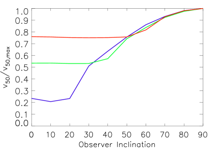
Figure 10: Simulated evolution of normalised $v_{50}$ with observer inclination (in ^∘, 0^∘ polar, 90^∘ equatorial view) for a ⁵⁶Ni/O disc with opening angles of $20^{\circ}$ (blue, lower line), $40^{\circ}$ (green, central line), and $60^{\circ}$ (red, upper line). Opening angles of only $20^{\circ}$ would cause very low projected velocities, which seem not to be observed. Opening angles between $40^{\circ}$ and $60^{\circ}$ seem to be able to explain the observed range of projected velocities, and are consistent with the distribution of high and low characteristic BL-SNe (see Figure 3).

6 Summary and Conclusions

We estimated ⁵⁶Ni masses for 29 SNe for which ⁵⁶Ni masses were not previously known. Their average agrees with the average of 18 CC-SN ⁵⁶Ni masses estimated before rather well, however there might be a small systematic over-estimate of the ⁵⁶Ni mass in this work. Individual estimates might be quite erroneous given the poor quality of the data set. We then measured characteristic velocities for 56 CC-SN cores, which range from 3000 km s^-1 to 7000 km s^-1 ($v_{\alpha}$). Several BL-SNe with high-velocity outer ejecta have high-velocity cores as well, but some BL-SNe do not. We have shown that this might be due to ejecta asphericities, which are expected theoretically and might have been detected by different methods before. We found that the average core velocities of SNe IIb are slightly lower than core velocities of SNe Ib and SNe Ic. SNe Ib and Ic have very similar average core velocities. SNe IIb show much less variance ($\sigma_{v}\approx 400$ km s^-1) of their core velocities than SNe Ib and Ic ($\sigma_{v}\approx 850$ km s^-1).

There seems to be no strong dependence of core velocity on ⁵⁶Ni mass. We also checked for correlations between total ejecta mass or kinetic energy and the core velocity and found none. There is only a weak correlation between the ratio of total kinetic energy to total mass and the core velocity (BL-SNe have the highest core velocities on average, but the scatter is so large that there is almost no predictive power). Therefore, although the total mass of a SN might be estimated (if the spectrum is flux calibrated), it is not possible to estimate the SN total kinetic energy from a nebular spectrum with good accuracy, since the core velocity seems to correlate with the outer ejecta velocities only weakly. We will further study the relation between outer and inner ejecta velocities in future work.

The uncertainties in our estimates are rather large. They are caused by the general properties of our method (background subtraction, reddening, time evolution of line width, uncertainty on epoch, ⁵⁶Ni distribution, and ⁵⁶Ni mass) and are difficult to improve upon when only limited high-quality data are available that cover different CC-SNe at several different epochs. Therefore more and better data is needed.

Appendix A

In CC-SNe nebular spectra, the [O I] $\lambda\lambda$6300, 6364 doublet often has a double or even triple peaked emission profile. Recently, Milisavljevic et al. (2009) studied these peaks for 20 CC-SNe and found that they are often separated by $\sim$64 Å. Since this coincides with the doublet separation, Milisavljevic et al. (2009) concluded that the multi-peaked line profiles might be caused by some absorption processes, rather than by ejecta geometry. In our sample there are 24 SNe with clear multi-peaked [O I] $\lambda\lambda$ 6300, 6364 profiles, and we measured their peak separation $\Delta$ (see Table 4).

For SNe 2004ao, 2005kl, 2006T, and 2008ax our results agree with those of Milisavljevic et al. (2009). For SN 2003jd, Milisavljevic et al. (2009) did not measure the separation of the two largest peaks, while we do, which explains the different value given in this paper.

Although about 50% of the SNe might be consistent with a separation of 64 Å(within the uncertainties), the other 50% are not. For SNe 1985F and 2002ap it seems likely that the second (very weak) peak is caused by the [O i] $\lambda$6364 line, since the first peak is roughly at 6300 Å while the second is at $\sim$6360 Å. For SNe 1990U, 1991aj, 2000ew, 2003jd, 2004ao, 2004gt, 2006T, 2007I, 2007bi, and 2008ax, the two peaks are of similar strength and are centered around 6300 Å. The separation observed in SNe 1990U, 1991aj, 2003jd, 2007I, and 2007bi is clearly not consistent with 64 Å. For the remaining 12 SNe the situation seems even less clear and we refer to Milisavljevic et al. (2009) for some possible explanations.

Interpreting the separation of these peaks as a geometrical effect, one obtains typical velocities between 2000 km s^-1 and 4000 km s^-1 (1000 km s^-1 to 2000 km s^-1 when considering half width) which is of the same order as the characteristic core velocities measured in this paper. Therefore the observed clustering around $\sim$ 3000 km s^-1 (close to the 64 Å doublet line separation) might be a coincidence caused by the typical velocity of the SNe cores.

In conclusion, one can say that ejecta geometry remains an interesting explanation for split-top line profiles.

SN	$\Delta$ [Å] (this work)	$\Delta$ [Å] Milisavljevic et al. (2009)
1985F	58 $\pm$ 4
1990B	65 $\pm$ 10 / 65 $\pm$ 10
1990U	48 $\pm$ 10
1990aa	45 $\pm$ 10 / 61 $\pm$ 6
1990aj	49 $\pm$ 6
1996N	65 $\pm$ 10
1996aq	63 $\pm$ 6
2000ew	59 $\pm$ 6
2002ap	58 $\pm$ 4
2003bg	38 $\pm$ 8
2003jd	100$\pm$ 20	64 $\pm$ 5
2004ao	64 $\pm$ 10	65 $\pm$ 3
2004dk	72 $\pm$ 10
2004gt	64 $\pm$ 8
2005N	50 $\pm$ 10
2005bf	50 $\pm$ 20
2005kl	65 $\pm$ 10	65 $\pm$ 4
2006ld	42 $\pm$ 6 / 61 $\pm$ 8
2006T	70 $\pm$ 20	63 $\pm$ 3
2007C	52 $\pm$ 10 / 50 $\pm$ 10
2007I	45 $\pm$ 10
2007bi	47 $\pm$ 6
2008D	45 $\pm$ 10
2008ax	61 $\pm$ 4	64 $\pm$ 1

Table 4: Peak separation measured in this work and by Milisavljevic et al. (2009). Two values are given if three peaks are observed; the separation is then measured from one peak to the next. For all SNe but SN 2003jd the estimates agree rather well. For SN 2003jd the difference is caused by the fact that Milisavljevic et al. (2009) did not measure the separation of the two largest peaks.

References

- Axelrod (1980) Axelrod T. S., 1980, Ph.D. thesis, AA(California Univ., Santa Cruz.)
- Barkat et al. (1967) Barkat Z., Rakavy G., Sack N., 1967, Physical Review Letters, 18, 379
- Bartunov et al. (1994) Bartunov O. S., Blinnikov S. I., Pavlyuk N. N., Tsvetkov D. Y., 1994, A&A, 281, L53
- Begelman & Sarazin (1986) Begelman M. C., Sarazin C. L., 1986, ApJ, 302, L59
- Blondin et al. (2003) Blondin J. M., Mezzacappa A., DeMarino C., 2003, ApJ, 584, 971
- Blondin & Calkins (2008) Blondin S., Calkins M., 2008, Central Bureau Electronic Telegrams, 1191, 2
- Brown et al. (2008) Brown P. J., Immler S., The Swift Satellite Team, 2008, The Astronomer’s Telegram, 1403, 1
- Burrows et al. (2007) Burrows A., Livne E., Dessart L., Ott C. D., Murphy J., 2007, ApJ, 655, 416
- Chugai (1992) Chugai N. N., 1992, Soviet Astronomy Letters, 18, 239
- Clocchiatti et al. (2001) Clocchiatti A., Suntzeff N. B., Phillips M. M., et al., 2001, ApJ, 553, 886
- Clocchiatti & Wheeler (1997) Clocchiatti A., Wheeler J. C., 1997, in NATO ASIC Proc. 486: Thermonuclear Supernovae, edited by P. Ruiz-Lapuente, R. Canal, J. Isern, 863–+
- Clocchiatti et al. (1996) Clocchiatti A., Wheeler J. C., Benetti S., Frueh M., 1996, ApJ, 459, 547
- Deng et al. (2005) Deng J., Tominaga N., Mazzali P. A., Maeda K., Nomoto K., 2005, ApJ, 624, 898
- Dimai & Migliardi (2005) Dimai A., Migliardi M., 2005, Central Bureau Electronic Telegrams, 300, 1
- Dimai & Villi (2006) Dimai A., Villi M., 2006, Central Bureau Electronic Telegrams, 364, 1
- Drissen et al. (1996) Drissen L., Robert C., Dutil Y., et al., 1996, IAU Circ., 6317, 2
- Elias et al. (1990) Elias J., Phillips M., Suntzeff N., 1990, IAU Circ., 5080, 2
- Elmhamdi et al. (2004) Elmhamdi A., Danziger I. J., Cappellaro E., et al., 2004, A&A, 426, 963
- Filippenko (1988) Filippenko A. V., 1988, AJ, 96, 1941
- Filippenko (1997) Filippenko A. V., 1997, ARA&A, 35, 309
- Filippenko & Korth (1991) Filippenko A. V., Korth S., 1991, IAU Circ., 5234, 1
- Frieman (2006) Frieman J., 2006, IAU Circ., 8766, 1
- Gabrijelcic et al. (1997) Gabrijelcic A., Benetti S., Lidman C., 1997, IAU Circ., 6535, 1
- Galama et al. (1999) Galama T. J., Vreeswijk P. M., van Paradijs J., et al., 1999, A&AS, 138, 465
- Gomez & Lopez (1994) Gomez G., Lopez R., 1994, AJ, 108, 195
- Graham & Li (2004) Graham J., Li W., 2004, Central Bureau Electronic Telegrams, 75, 1
- Hamuy et al. (2009) Hamuy M., Deng J., Mazzali P. A., et al., 2009, ArXiv e-prints
- Heger & Woosley (2005) Heger A., Woosley S., 2005, in From Lithium to Uranium: Elemental Tracers of Early Cosmic Evolution, edited by V. Hill, P. François, F. Primas, vol. 228 of IAU Symposium, 297–302
- Hoflich (1991) Hoflich P., 1991, A&A, 246, 481
- Itagaki et al. (2006) Itagaki K., Nakano S., Puckett T., Toth D., 2006, IAU Circ., 8751, 2
- Janka et al. (2007) Janka H.-T., Langanke K., Marek A., Martínez-Pinedo G., Müller B., 2007, Phys. Rep., 442, 38
- Jin et al. (2007) Jin C. C., Cao Y., Bian F.-Y., et al., 2007, IAU Circ., 8798, 1
- Kotake et al. (2004) Kotake K., Sawai H., Yamada S., Sato K., 2004, ApJ, 608, 391
- Li & McCray (1992) Li H., McCray R., 1992, ApJ, 387, 309
- Maeda et al. (2008) Maeda K., Kawabata K., Mazzali P. A., et al., 2008, Science, 319, 1220
- Maeda et al. (2007a) Maeda K., Kawabata K., Tanaka M., et al., 2007a, ApJ, 658, L5
- Maeda et al. (2002) Maeda K., Nakamura T., Nomoto K., Mazzali P. A., Patat F., Hachisu I., 2002, ApJ, 565, 405
- Maeda et al. (2007b) Maeda K., Tanaka M., Nomoto K., et al., 2007b, ApJ, 666, 1069
- Malesani et al. (2004) Malesani D., Tagliaferri G., Chincarini G., et al., 2004, ApJ, 609, L5
- Matheson (2004) Matheson T., 2004, in Cosmic explosions in three dimensions, edited by P. Höflich, P. Kumar, J. C. Wheeler, 351–+
- Matheson et al. (2001) Matheson T., Filippenko A. V., Li W., Leonard D. C., Shields J. C., 2001, AJ, 121, 1648
- Maund et al. (2005) Maund J. R., Smartt S. J., Schweizer F., 2005, ApJ, 630, L33
- Mazzali et al. (2002) Mazzali P. A., Deng J., Maeda K., et al., 2002, ApJ, 572, L61
- Mazzali et al. (2004) Mazzali P. A., Deng J., Maeda K., Nomoto K., Filippenko A. V., Matheson T., 2004, ApJ, 614, 858
- Mazzali et al. (2006) Mazzali P. A., Deng J., Nomoto K., et al., 2006, Nature, 442, 1018
- Mazzali et al. (2005) Mazzali P. A., Kawabata K. S., Maeda K., et al., 2005, Science, 308, 1284
- Mazzali et al. (2007a) Mazzali P. A., Kawabata K. S., Maeda K., et al., 2007a, ApJ, 670, 592
- Mazzali et al. (2001) Mazzali P. A., Nomoto K., Patat F., Maeda K., 2001, ApJ, 559, 1047
- Mazzali et al. (2007b) Mazzali P. A., Röpke F. K., Benetti S., Hillebrandt W., 2007b, Science, 315, 825
- Mazzali et al. (2008) Mazzali P. A., Valenti S., Della Valle M., et al., 2008, Science, 321, 1185
- McNaught et al. (1991) McNaught R. H., della Valle M., Pasquini L., 1991, IAU Circ., 5178, 1
- Milisavljevic et al. (2009) Milisavljevic D., Fesen R., Gerardy C., Kirshner R., Challis P., 2009, ArXiv e-prints
- Modjaz et al. (2008) Modjaz M., Kirshner R. P., Blondin S., Challis P., Matheson T., 2008, ApJ, 687, L9
- Modjaz et al. (2009) Modjaz M., Li W., Butler N., et al., 2009, ApJ, 702, 226
- Moiseenko et al. (2006) Moiseenko S. G., Bisnovatyi-Kogan G. S., Ardeljan N. V., 2006, MNRAS, 370, 501
- Monard (2006) Monard L. A. G., 2006, IAU Circ., 8666, 2
- Monard et al. (2004) Monard L. A. G., Quimby R., Gerardy C., et al., 2004, IAU Circ., 8454, 1
- Nakamura et al. (2000) Nakamura T., Maeda K., Iwamoto K., et al., 2000, in Highly Energetic Physical Processes and Mechanisms for Emission from Astrophysical Plasmas, edited by P. C. H. Martens, S. Tsuruta, M. A. Weber, vol. 195 of IAU Symposium, 347–+
- Nakano et al. (1996) Nakano S., Aoki M., Kushida R., et al., 1996, IAU Circ., 6454, 1
- Nakano et al. (1997) Nakano S., Aoki M., Kushida Y., et al., 1997, IAU Circ., 6552, 1
- Nomoto et al. (1990) Nomoto K., Shigeyama T., Filippenko A. V., 1990, vol. 22 of Bulletin of the American Astronomical Society, 1221–+
- Nomoto et al. (1993) Nomoto K., Suzuki T., Shigeyama T., Kumagai S., Yamaoka H., Saio H., 1993, Nature, 364, 507
- Nugent (2007) Nugent P. E., 2007, Central Bureau Electronic Telegrams, 929, 1
- Parisky & Li (2007) Parisky X., Li W., 2007, Central Bureau Electronic Telegrams, 1158, 1
- Pastorello et al. (2008) Pastorello A., Kasliwal M. M., Crockett R. M., et al., 2008, MNRAS, 389, 955
- Perlmutter et al. (1990) Perlmutter S., Pennypacker C., Carlson S., Marvin H., Muller R., Smith C., 1990, IAU Circ., 5087, 1
- Pian et al. (2006) Pian E., Mazzali P. A., Masetti N., et al., 2006, Nature, 442, 1011
- Pollas & Maury (1991) Pollas C., Maury A., 1991, IAU Circ., 5200, 1
- Puckett et al. (2000) Puckett T., Langoussis A., Garradd G. J., 2000, IAU Circ., 7530, 1
- Puckett et al. (2007) Puckett T., Orff T., Madison D., et al., 2007, IAU Circ., 8792, 2
- Pugh et al. (2004) Pugh H., Li W., Manzini F., Behrend R., 2004, IAU Circ., 8452, 2
- Quimby et al. (2004) Quimby R., Gerardy C., Hoeflich P., et al., 2004, IAU Circ., 8446, 1
- Quimby et al. (2007) Quimby R., Odewahn S. C., Terrazas E., Rau A., Ofek E. O., 2007, Central Bureau Electronic Telegrams, 953, 1
- Sahu et al. (2009) Sahu D. K., Tanaka M., Anupama G. C., Gurugubelli U. K., Nomoto K., 2009, ApJ, 697, 676
- Sauer et al. (2006) Sauer D. N., Mazzali P. A., Deng J., Valenti S., Nomoto K., Filippenko A. V., 2006, MNRAS, 369, 1939
- Scannapieco et al. (2005) Scannapieco E., Madau P., Woosley S., Heger A., Ferrara A., 2005, ApJ, 633, 1031
- Schlegel et al. (1998) Schlegel D. J., Finkbeiner D. P., Davis M., 1998, ApJ, 500, 525
- Schmidt et al. (2005) Schmidt B., Salvo M., Wood P., 2005, IAU Circ., 8472, 2
- Silverman et al. (2009a) Silverman J. M., Mazzali P., Chornock R., et al., 2009a, ArXiv e-prints
- Silverman et al. (2009b) Silverman J. M., Mazzali P., Chornock R., et al., 2009b, PASP, 121, 689
- Singer & Li (2004) Singer D., Li W., 2004, IAU Circ., 8299, 1
- Stritzinger et al. (2009) Stritzinger M., Mazzali P., Phillips M. M., et al., 2009, ApJ, 696, 713
- Stritzinger et al. (2006) Stritzinger M., Mazzali P. A., Sollerman J., Benetti S., 2006, A&A, 460, 793
- Takiwaki et al. (2009) Takiwaki T., Kotake K., Sato K., 2009, ApJ, 691, 1360
- Tanaka et al. (2007) Tanaka M., Maeda K., Mazzali P. A., Nomoto K., 2007, ApJ, 668, L19
- Taubenberger et al. (2006) Taubenberger S., Pastorello A., Mazzali P. A., et al., 2006, MNRAS, 371, 1459
- Taubenberger et al. (2005) Taubenberger S., Pastorello A., Mazzali P. A., Witham A., Guijarro A., 2005, Central Bureau Electronic Telegrams, 305, 1