Stochastic Processes Crossing from Ballistic to Fractional Diffusion with Memory: Exact Results

Abstract

We address the now classical problem of a diffusion process that crosses over from a ballistic behavior at short times to a fractional diffusion (sub- or super-diffusion) at longer times. Using the standard non-Markovian diffusion equation we demonstrate how to choose the memory kernel to exactly respect the two different asymptotics of the diffusion process. Having done so we solve for the probability distribution function (pdf) as a continuous function which evolves inside a ballistically expanding domain. This general solution agrees for long times with the pdf obtained within the continuous random walk approach but it is much superior to this solution at shorter times where the effect of the ballistic regime is crucial.

Introduction: Nature offers us a large number of examples of diffusion processes for which an observable $X$ diffuses in time such that its variance grows according to

$$\langle\Delta X^{2}\rangle(t)\sim D_{2}t^{2}\quad\mbox{for}~{}t\ll t_{c}\ ,$$ (1)

$$\langle\Delta X^{2}\rangle(t)\sim D_{\alpha}t^{\alpha}\quad\mbox{for}~{}t\gg t_{c}\ ,$$ (2)

where angular brackets mean an average over repeated experiments and $D_{2}$ and $D_{\alpha}$ are coefficients with the appropriate dimensionality. The short time behavior is known as ‘ballistic’, and is generic for a wide class of processes. The long time behavior with $\alpha\neq 1$ is generic when the diffusion steps are correlated, with persistence for $\alpha>1$ and anti-persistence for $\alpha<1$ MN68 . These correlations mean that the diffusion process is not Markovian, but rather has memory. Thus the probability distribution function (pdf) of the observable $X$, $f(X,t)$ is expected to satisfy a diffusion equation with memory KK74 ,

$$\frac{\partial f(X,t)}{\partial t}=\int_{0}^{t}dt^{\prime}K(t-t^{\prime})\nabla^{2}f(X,t)\ ,$$ (3)

with $K(t)$ being the memory kernel and $\nabla^{2}$ the Laplace operator.

In this Letter we study the class of processes which satisfy Eqs. (1)-(3). First of all we find an expression for the kernel $K(t)$ which is unique for a given law of mean-square-displacement. Second we consider the kernel which contains both the ballistic contribution embodied in Eq. (1) and the long-time behavior (2). For this case we find an exact equation and a solution for Eq. (3). Lastly a simple interpolation formula for the kernel is inserted to the exact equation which is then solved for the pdf of $X$ without any need for the fractional dynamics approach MK00 . Some interesting characteristics of the solution are described below.

Determination of the kernel $K(t)$: To determine the kernel in Eq. (3) we use a result obtained in S02 . Consider the auxiliary equation

$$\frac{\partial P(X,t)}{\partial t}=\nabla^{2}P(X,t)\ .$$ (4)

Define the Laplace transform of the solution of Eq. (4) as

$$\tilde{P}(X,s)\equiv\int_{0}^{t}{\rm d}te^{-st}P(X,t)\ ,$$ (5)

it was shown in S02 that the solution of Eq. (3) with the same initial conditions can be written as

$$\tilde{f}(X,s)=\frac{1}{\tilde{K}(s)}\tilde{P}(X,\frac{s}{\tilde{K}(s)})\ ,$$ (6)

where here and below the tilde above the symbol means the Laplace transform. The development that we propose here is to replace in Eq. (6) the Laplace transform $\tilde{K}(s)$ with the Laplace transform of the mean-square displacement. This is done by first realizing (by computing the variance and integrating by parts) that

$$\frac{\partial\langle X^{2}\rangle(t)}{\partial t}=2\int_{0}^{t}{\rm d}t^{\prime}K(t-t^{\prime})\ ,$$ (7)

or, equivalently,

$$\tilde{K}(s) = \frac{s^{2}\widetilde{\langle{X^{2}}\rangle}(s)}{2}\ ,$$

$$= \frac{\partial\langle X^{2}\rangle(t)}{2\partial t}+\frac{s}{2}\widetilde{\frac{\partial\langle X^{2}\rangle(t)}{\partial t}}-\frac{\partial\langle X^{2}\rangle(t)}{2\partial t}\ .$$

The second line was written in order to find the time representation of $K(t)$ which is the inverse Laplace transform:

$$K(t) = \frac{1}{2}\Bigg{(}\delta(t)\frac{\partial}{\partial t}\langle X^{2}\rangle(t)+\frac{\partial^{2}}{\partial t^{2}}\langle X^{2}\rangle(t)\Bigg{)}$$ (9)

$$= \frac{1}{2}\frac{\partial}{\partial t}\Bigg{(}H(t)\frac{\partial\langle X^{2}\rangle(t)}{\partial t}\Bigg{)}\ ,$$

where $H(t)$ is the Heaviside function. Obviously, using the first line of Eq. (Stochastic Processes Crossing from Ballistic to Fractional Diffusion with Memory: Exact Results) in Eq. (6) the solution is entirely determined by whatever law is given for the variance, together with initial conditions.

For ordinary diffusion the variance is defined by Eq. (2) with $\alpha=1$ and $t_{c}=0$. It follows from Eq. (9) that the kernel is $K(t)\sim\delta(t)$ and Eq. (3) is reduced to the Markovian Eq. (4); this process does not possess any memory. More complicated examples are considered below.

Example I: fractional differential equations. In recent literature the problem of a diffusion process which is consistent with Eq. (2) only for all times (i.e. $t_{c}=0$) is investigated using the formalism of fractional differential equations (see, e.g., MK00 ). In this formalism Eq. (3) is replaced by the fractional equation

$$\frac{\partial f(X,t)}{\partial t}=D_{\alpha}\hskip 2.84526pt{}_{0}\mathrm{\bf D}^{1-\alpha}_{t}\frac{\partial^{2}f(X,t)}{\partial x^{2}},$$ (10)

where the Rieman-Liouville operator ${}_{0}\mathrm{\bf D}^{1-\alpha}_{t}$ is defined by

$${}_{0}\mathrm{\bf D}^{1-\alpha}_{t}\phi(x,t)=\frac{1}{\Gamma(\alpha)}\frac{\partial}{\partial t}\int_{0}^{t}{\rm d}t^{\prime}\frac{\phi(x,t^{\prime})}{(t-t^{\prime})^{1-\alpha}},$$ (11)

where $\Gamma(\alpha)$ is the gamma function. It is easy to see that this equation follows from Eq. (3) with the kernel evaluated by Eq. (9) with the variance (2). We reiterate however that this equation is consistent with Eq. (2) for all times $t\geq 0$. This of course is a problem since this formalism cannot agree with the ballistic short time behavior which is generic in many systems.

Example II: ballistic behavior. For $X$ one-dimensional the solution of Eq. (4) with the initial condition $P(X,t=0)=\delta(X)$ is given by

$$\tilde{P}(X,s)=\frac{1}{2\sqrt{s}}\cdot\exp(-\mid X\mid\sqrt{s})\ .$$ (12)

Substituting in Eq. (6) we find

$$\tilde{f}(X,s)=\frac{1}{\sqrt{2s^{3}\widetilde{\langle X^{2}\rangle}(s)}}\exp(-\mid X\mid\sqrt{\frac{2}{s\widetilde{\langle X^{2}\rangle}(s)}}).$$ (13)

For systems with the pure ballistic behavior (e.g., dilute gas) the variance can be written as $\langle X^{2}\rangle_{t}=\langle u^{2}\rangle t^{2}$, where $\langle u^{2}\rangle$ is the mean square average of the particle velocities. The Laplace transform of this expression is given by $\widetilde{\langle X^{2}\rangle}(s)=2\langle u^{2}\rangle/s^{3}$ and the Laplace transform of the pdf is defined by

$$\tilde{f}(X,s)=\frac{1}{2\sqrt{\langle u^{2}\rangle}}~{}\exp(-\mid X\mid\frac{s}{\sqrt{\langle u^{2}\rangle}})\ .$$ (14)

The inverse transform reads

$$f(X,t)=\frac{1}{2}\delta(\mid X\mid-\sqrt{\langle u^{2}\rangle}t)\ .$$ (15)

This solution corresponds to a deterministic evolution; there is a complete memory of the initial conditions in the absence of inter-particle interactions, $K(t)=\langle u^{2}\rangle$).

General case: In the general case the mean-square-displacement satisfied some law $\langle X^{2}\rangle(t)$ which is supposed to be known at all times, with possible asymptotic behavior as shown in Eqs. (1) and(2). To find the appropriate general solution we will split $\tilde{f}(X,s)$ into two parts, $\tilde{f}_{I}(X,s)$ and $\tilde{f}_{II}(X,s)$, such that the first part is constructed to agree with the existence of a ballistic regime. Suppose that in that regime, at short time, the mean-square-displacement can be expanded in a Taylor series

$$\langle X^{2}\rangle(t)=\sum_{i=0}^{\infty}a_{i}t^{\mu_{i}-1}\ =a_{0}t^{2}+a_{1}t^{3}+a_{2}t^{4}\cdots\ ,$$ (16)

where $\mu_{0}=3$, $\mu_{1}=4$ etc. Then the Laplace transform $\widetilde{\langle X^{2}\rangle}(s)$ can be written for $s\to\infty$ as PB64

$$\widetilde{\langle X^{2}\rangle}(s)=\sum_{i=0}^{\infty}a_{i}\Gamma(\mu_{i})\frac{1}{s^{\mu_{i}}}=2a_{0}\frac{1}{s^{3}}+6a_{1}\frac{1}{s^{4}}+24a_{2}\frac{1}{s^{5}}\cdots\ .$$ (17)

Substituting Eq. (17) up to O$(s^{-4})$ in Eq. (13) yields

$$\tilde{f}_{I}(X,s)_{s\to\infty}=\frac{1}{2\sqrt{a_{0}}}exp(-\frac{\mid X\mid}{\sqrt{a_{0}}}(s-\frac{3a_{1}}{2a_{0}}))\ .$$ (18)

The inverse Laplace transform of this result reads

$$f_{I}(X,t)=\frac{1}{2}exp(\frac{3a_{1}}{2a_{0}}t)\delta(\mid X\mid-\sqrt{a_{0}}t)\ .$$ (19)

Not surprisingly, this partial solution corresponds to a deterministic propagation. Note that in order to avoid exponential divergence in time we must have $a_{1}<0$ in the expansion (16).

Having found $\tilde{f}_{I}(X,s)$ we can now write $\tilde{f}_{II}(X,s)$ simply as

$$\tilde{f}_{II}(X,s)=\tilde{f}(X,s)-\tilde{f}_{I}(X,s)\ .$$ (20)

Calculating this difference explicitly we find

$$\tilde{f}_{II}(X,s) = \frac{1}{2}\Bigg{(}\sqrt{\frac{2}{s^{3}\widetilde{\langle X^{2}\rangle}(s))}}\exp(-\mid X\mid(\sqrt{\frac{2}{s\widetilde{\langle X^{2}\rangle}(s)}}-\frac{s}{\sqrt{a_{0}}}))-\frac{1}{\sqrt{a_{0}}}\exp(\frac{3a_{1}}{2a_{0}^{3/2}}\mid X\mid)\Bigg{)}\exp(-\frac{\mid X\mid}{\sqrt{a_{0}}}s)$$ (21)

$$\equiv \tilde{F}(X,s)\exp(-\frac{\mid X\mid}{\sqrt{a_{0}}}s).$$

The inverse Laplace transform of Eq. (21) is given by

$$f_{II}(X,t)=F\Big{(}X,t-{\mid X\mid}/{\sqrt{a_{0}}}\Big{)}H(\sqrt{a_{0}}t-\mid X\mid).$$ (22)

The importance of this result is that the explicit Heaviside function is taking upon itself the discontinuity in the solution $f_{II}(X,t)$. The exact value of this function at the point $\mid X\mid=\sqrt{a_{0}}t$ can be calculated using the initial value theorem and is given by

$$f_{II}(\mid X\mid=\sqrt{a_{0}}t,t)=$$ (23)

$$-\Bigg{(}\frac{3}{4}\frac{a_{1}}{a_{0}^{3/2}}+\frac{1}{2\sqrt{a_{0}}}(\frac{27}{8}[\frac{a_{1}}{a_{0}}]^{2}-6\frac{a_{2}}{a_{0}})t\Bigg{)}\times\exp(-\frac{3}{2}\frac{a_{1}}{a_{0}}t)\ .$$

Summing together the results (19) and (22) in the time domain we get a general solution of the non-Markovian problem with a short-time ballistic behavior, in the form

$$f(X,t) = \frac{1}{2}exp(\frac{3a_{1}}{2a_{0}}t)\delta(\mid X\mid-\sqrt{a_{0}}t)$$ (24)

$$+ F(X,t-\frac{\mid X\mid}{\sqrt{a_{0}}})H(\sqrt{a_{0}}t-\mid X\mid).$$

This is the main result of the present Letter. The diffusion repartition of the probability distribution function occurs inside the spatial diffusion domain which increases in a deterministic way.

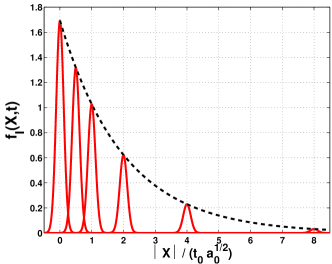
Figure 1: The time evolution of the function $f_{I}(X,t)$ defined by Eq. (19) for time intervals $t/t_{0}=$0.5, 1, 2, 4, 8 (the time scale $t_{0}=a_{0}/(3a_{1})$). The $\delta$-function is graphically represented by narrow Gaussians.

The first term in Eq. (24) corresponds to the propagating $\delta$-function which is inherited from the initial conditions, and it lives at the edge of the ballistically expanding domain. Schematically the time evolution of this term is shown in Fig.1, where the $\delta$-function is graphically represented as a narrow Gaussian. The dashed line represents the exponential decay of the integral over the $\delta$-function. The function $F(X,t-\frac{\mid X\mid}{\sqrt{a_{0}}})$ in the time domain is a continuous function and can be evaluated numerically, for example using the direct integration method duf93 . Below we demonstrate this calculation with explicit examples.

Interpolation for all times: To interpolate Eqs. (1) and (2) we propose the form

$$\langle\Delta X^{2}\rangle_{t}=2D_{\alpha}t_{0}^{\alpha}\frac{(t/t_{0})^{2}}{(1+(t/t_{0}))^{2-\alpha}},$$ (25)

where $0\leq\alpha\leq 2$. Here $t_{0}$ is the crossover characteristic time, at $t\ll t_{0}$ the law (25) describes the ballistic regime and at $t\gg t_{0}$ the fractional diffusion.

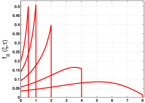
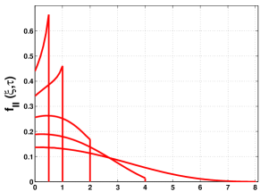
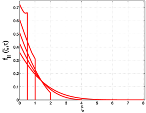
Figure 2: The continuous part of the pdf (22) for different values of the parameter $\alpha$. Superdiffusion ($\alpha=3/2$, upper panel), regular diffusion ($\alpha=1$, middle panel) and subdiffusion ($\alpha=1/2$, lower panel). Time intervals from the top to the bottom $\tau=$0.5, 1, 2, 4, 8. The reader should note that the full solution of the problem is the sum of the two solutions shown in this and the previous figure.

Introduce now dimensionless variables $\langle\xi^{2}\rangle_{\tau}=\langle\Delta X^{2}\rangle_{t}/(2D_{\alpha}t_{0}^{\alpha})$ and $\tau=t/t_{0}$. With these variables the last equation reads

$$\langle\xi^{2}\rangle_{\tau}=\frac{\tau^{2}}{(1+\tau)^{2-\alpha}}.$$ (26)

The Taylor expansion of (25) is given by

$$\langle\xi^{2}\rangle_{\tau}=\tau^{2}-(2-\alpha)\tau^{3}+\frac{1}{2}(3-\alpha)(2-\alpha)\tau^{4}+\ldots.$$ (27)

Substitution these expansion coefficients into Eq. (19) yields the first term in the expression for the probability distribution function (24)

$$f_{I}(x,t)=\frac{1}{2}exp(-\frac{3(2-\alpha)}{2}\tau)\delta(\mid\xi\mid-\tau).$$ (28)

The Laplace transform of Eq. (26) is

$$\widetilde{\langle X^{2}\rangle}(s)=(\frac{\alpha}{s}-1)\frac{1}{s}+\bigg{(}(\alpha-1)(\frac{\alpha}{s}-2)+s\bigg{)}\frac{e^{s}}{s^{\alpha}}\Gamma(\alpha-1,s),$$ (29)

where $\Gamma(a,s)$ is the incomplete gamma function. Note that the case $\alpha=2$ is special, since it annuls the exponent in Eq. (28), leaving as a solution a ballistically propagating $\delta$-function. For all other values of $\alpha<2$ the inverse Laplace transform of the function $\widetilde{F}(x,s)$ which defines the diffusion process inside the expanded spatial domain should be evaluated, in general, numerically.

Results of the calculations following the method of Ref. duf93 for the smooth part of the probability distribution function $f_{II}(x,t)$ for different values of the parameter $\alpha$ are shown in Fig. 2. The reader should appreciate the tremendous role of memory, or the non-Markovian nature of the process under study. For example regular diffusion with $\alpha=1$ results in a Gaussian pdf that is peacefully expanding and flattening as time increases. Here, in the mid panel of Fig. 2 we see that the ballistic part which is represented by the advancing and reducing $\delta$-function sends backwards the probability that it loses due to the exponential decay seen in Fig. 1. This ‘back-diffusion’ leads initially to a qualitatively different looking pdf, with a maximum at the edge of the ballistically expanding domain. At later times the pdf begins to resemble more regular diffusion. The effect strongly depends on $\alpha$ simply due to the appearance of $\alpha$ in the exponent in Eq. (28).

For long times the solutions shown in Fig. 2 agree with the Markovian pdf obtained in the frame of a continuous-time random walk BHW87 . For the special case $\alpha=0$ the limiting behavior of the general solution from Eq. (24) can be evaluated with the help of the final value theorem:

$$f(X)=\frac{1}{\sqrt{2}}\exp(-\sqrt{2}\mid X\mid),$$ (30)

this analytical result coincides with the pdf from BHW87 at the same conditions.

In summary, we have shown how to deal with diffusion processes that cross-over from a ballistic to a fractional behavior for short and long times respectively, within the time non-local approach. The general solution (24) demonstrates the effect of the temporal memory in the form of a partition of the probability distribution function inside a spatial domain which increases in a deterministic way. The approach provides a solution that is valid at all times, and in particular is free from the instantaneous action puzzle.

References

• (1) B. B. Mandelbrot, J. W. van Ness, Fractional Brownian Motions, Fractional Noises and Applications. SIAM Rev. 10, 422-437 (1968).
• (2) V. M. Kenkre, R. S. Knox, Generalized-master-equation theory of excitation transfer. Phys. Rev. B 9, 5279-5290 (1974).
• (3) R. Metzler, J. Klafter, The Random Walk’s Guide to Anomalous Diffusion: a Fractional Dynamics Approach. Phys. Rep. 339, 1-77 (2000).
• (4) I.M.Sokolov. Solution of a Class of Non-Markovian Fokker-Plank Equations. Phys. Rev. E 66, 41101-41105 (2002).
• (5) B. van der Pol, H. Bremmer, Operational Calculus. Univ. Press, Cambrige (1964).
• (6) D.G.Duffy. Numerical Inversion of the Laplace Transform: Comparison of Three New Methods on Characteristic Problems from Applications. ACM TOMS 19, pp.335-359 (1993).
• (7) R. C. Ball, S. Havlin, G. H. Weiss, Non-Gaussian Random Walks. J. Phys. A: Math. Gen., 20, 4055-4059 (1987).