The VIMOS VLT Deep Survey: the group catalogue

Abstract

Aims. We present a homogeneous and complete catalogue of optical groups identified in the purely flux limited ($17.5\leq I_{AB}\leq 24.0$) VIMOS-VLT Deep redshift Survey (VVDS).

Methods. We use mock catalogues extracted from the MILLENNIUM simulation, to correct for potential systematics that might affect the overall distribution as well as the individual properties of the identified systems. Simulated samples allow us to forecast the number and properties of groups that can be potentially found in a survey with VVDS-like selection functions. We use them to correct for the expected incompleteness and also to asses how well galaxy redshifts trace the line-of-sight velocity dispersion of the underlying mass overdensity. In particular, we train on these mock catalogues the adopted group-finding technique i.e. the Voronoi-Delaunay Method (VDM). The goal is to fine-tune its free parameters, recover in a robust and unbiased way the redshift and velocity dispersion distributions of groups ($n(z)$ and $n(\sigma)$ respectively) and maximize, at the same time, the level of completeness and purity of the group catalogue.

Results. We identify 318 VVDS groups with at least 2 members in the range $0.2\leq z\leq 1.0$, among which 144 (/30) with at least 3 (/5) members. The sample has an overall completeness of $\sim 60$% and purity of $\sim 50$%. Nearly $45$% of the groups with at least 3 members are still recovered if we run the algorithm with the particular parameter set which maximizes the purity ($\sim 75$%) of the resulting catalogue. We exploit the group sample to explore the redshift evolution of the fraction $f_{b}$ of blue galaxies ($U-B\leq 1$) in the redshift range $0.2\leq z\leq 1$. We find that the fraction of blue galaxies is significantly lower in groups than in the global population (i.e. in the whole ensemble of galaxies irrespectively of their environment). Both of these quantities increase with redshift, with the fraction of blue galaxies in groups showing a marginally significant steeper increase. We also investigate the dependence of $f_{b}$ on group richness: not only we confirm that, at any redshift, the blue fraction decreases in systems with increasing richness, but we extend towards fainter luminosities the magnitude range over which this result holds.

1 Introduction

Galaxy groups and clusters are the largest and most massive gravitationally bound systems in the universe. Because of this, they are very useful cosmological probes. For example, the evolution of their abundance or baryon fraction give insights into the value of fundamental cosmological parameters (e.g. Borgani et al., 1999; Newman & Davis, 2002; Allen et al., 2002; Ettori et al., 2003; Zhang et al., 2006; Ettori et al., 2009), their mass and luminosity functions fix the amplitude of the power spectrum at cluster scales (e.g. Rosati et al., 2002; Finoguenov et al., 2010), while their optical mass-to-light ratio allows to constrain the matter density parameter $\Omega_{m}$ (e.g. Girardi et al., 2000; Marinoni & Hudson, 2002; Sheldon et al., 2009). Groups and clusters are also ideal laboratories for astrophysical studies. Several interesting physical processes are indeed triggered on scales characterized by such extreme density conditions. Their analysis is crucial in particular to understand the effects of local environment on galaxy formation and evolution (e.g. Oemler, 1974; Dressler, 1980; Postman & Geller, 1984; Dressler et al., 1997; Garilli et al., 1999; Treu et al., 2003; Poggianti et al., 2006).

1.1 The detection of galaxy groups and clusters

A whole arsenal of algorithms allows to identify and reconstruct galaxy systems. They range from the very first pioneer methods based on visual identification on photometric plates (Abell, 1958; Zwicky et al., 1968) to more recent techniques which exploit various physical properties of the systems as a guide for identification. For example, the thermal bremsstrahlung emission from the hot intracluster gas trapped inside the cluster gravitational potential allows to spot them by means of X-ray band observations. On the opposite side of the spectrum, in the centimetre regime, cluster detection is made possible thanks to the Sunyaev-Zeldovich effect (SZE, Sunyaev & Zeldovich, 1972, 1980). Indeed, the hot intracluster gas, by inverse-compton scattering the photons of the Cosmic Microwave Background (CMB), leaves a characteristic imprint in the CMB spectrum which can be exploited as a useful signature for identification. A cluster potential well can also be detected through strong gravitational lensing or the cosmic shear induced by weak gravitational lensing (Kneib et al., 2003; Gavazzi et al., 2009; Limousin et al., 2009; Richard et al., 2010; Limousin et al., 2010; Morandi et al., 2010). Clusters identification can be based also on the properties of the member galaxies. It has been observed that cluster cores host typically red galaxies, among which there are the brightest cluster galaxies (BCG). Thus, a cluster center can be identified as a R.A.-dec concentration of galaxies with typical red colours (see for example the Red-Sequence Cluster Survey, Gladders & Yee, 2000, the first cluster survey based on this method), in some case adding also the constraint of a high luminosity (e.g. the maxBCG method, Hansen et al., 2005, Koester et al., 2007).

An orthogonal approach, based on geometrical algorithms, consists in identifying systems from the 3D spatial distribution properties of their members. These algorithms vary from the earlier hierarchical method (Materne, 1978, Tully, 1980) and the widely used ‘friend of friend’ (FOF) method (Huchra & Geller, 1982), to the more recent 3D adaptive matched filter method (Kepner et al., 1999), the ‘C4’ method (Miller et al., 2005) and the Voronoi-Delaunay Method (VDM, Marinoni et al., 2002). Finally, group-finding algorithms have also been developed which exploit information extracted from photometric redshifts (e.g. Adami et al., 2005; Mazure et al., 2007).

The availability of several identification protocols is not only useful in order to confirm clusters detection by an a-posteriori cross-correlation of various independent catalogues, but it is also crucial for spotting eventual systematics which might affect individual detection techniques. For example, it has been shown by the first joint X-ray/optical survey (Donahue et al., 2002) that only $\sim$ 20% of the optically selected clusters were also identified in X-rays, while $\sim$60% of the X-ray clusters were detected in the optical sample. Understanding the possible selection effects hidden behind the different survey strategies is crucial in order to interpret this small overlap between the two different cluster catalogues (see for example Ledlow et al., 2003; Gilbank et al., 2004). Moreover, using the RASS-SDSS galaxy cluster catalogue Popesso et al. (2004) show that a distinct class of ‘X-ray underluminous Abell clusters’ does exist, with an X-ray luminosity $L_{X}$ which is one order of magnitude fainter than the one expected for their mass according to the typical $L_{X}$-mass relation (Popesso et al., 2007a). This supports the concern of Donahue et al. (2002) about the possible existence of biases in catalogues selected in different wavebands.

A major challenge we face is to extend cluster searches at high redshift. Indeed, most of the methods described above suffer from major drawbacks when applied in this regime. Both the X-ray apparent surface brightness and the gravitational lensing cross section of clusters decrease very rapidly with redshift. As a consequence, only very massive clusters can be detected at high $z$. On the contrary, the SZE detection efficiency does not depend on redshift, but large SZ survey are yet to be completed. For what concerns cluster detection using the spatial distribution of members, we emphasize the difference between photometric and spectroscopic galaxy data sets. Several methods have been proposed to detect clusters with photometric data, mainly exploiting galaxy colours in different bands. On the one side, this method has been successfully used both for surveys (see for example the above-mentioned Red-Sequence Cluster Survey, Gladders & Yee, 2000) and single detections (e.g. the very recent work by Andreon et al., 2009), but on the other hand the selection of red galaxies implies the selection of only the older structures, where galaxies lived enough time to be affected by the physical processes typical of the group environment (see for example the discussion in Gerke et al., 2007). Moreover, the depth required in photometric surveys to identify high-$z$ groups and clusters increases the number of foreground and background galaxies, due to the fact that objects surface number density is enhanced by the faint flux limit. This essentially limits the effectiveness of 2D identifications at high-$z$. The third dimensions is thus imperative if we want to disentangle in an efficient way projection effects. Nonetheless, the uncertainty on the line-of-sight position of galaxies may be a concern when it is bigger (or even much bigger) than the typical velocity dispersion of group galaxies, as in the case of photometric redshifts.

1.2 This work and the existing groups and clusters samples

To date, many local, optically selected group catalogues are available in literature. A review can be found in Eke et al. (2004), where one of the largest catalogue of galaxy groups detected in redshift space from the Two Degree Field Galaxy Redshift Survey (2dFGRS) is presented. Similarly, several group catalogues have been extracted from the Sloan Digital Sky Survey data (e.g. Miller et al., 2005; Berlind et al., 2006; Weinmann et al., 2006). Systematic searches of groups in redshift space have been undertaken also at intermediate redshift (e.g. within the CNOC2 survey, up to redshift $z=0.55$, Carlberg et al., 2001). The compilation of optically selected and complete samples of groups up to $z\sim 1$ and beyond has been made possible only recently thanks to the completion of large and deep spectroscopic surveys, such as the DEEP2 Galaxy Redshift Survey (Davis et al., 2003), the VIMOS-VLT Deep Survey (Le Fèvre et al., 2005), and the zCOSMOS survey (Lilly et al., 2007, 2009).

Gerke et al. (2005) present the first DEEP2 group catalogue: it contains 899 groups with two or more members identified in the redshift range $0.7\leq z\leq 1.4$ with the VDM method. The DEEP2 sample reaches a limiting magnitude of $R_{AB}=24.1$, and its galaxies are pre-selected in colour before being targeted for spectroscopic observations, in order to reduce the number of galaxies at $z\lesssim 0.7$. The first zCOSMOS group catalogue (Knobel et al., 2009) comprises $\sim 800$ groups with at least 2 members, covering the redshift range $0.1\leq z\leq 1.0$. The parent galaxy sample is purely flux limited ($15\leq I_{AB}\leq 22.5$), and groups are detected with the FOF method, combined with the VDM.

In this work, we make use of the VIMOS-VLT Deep Survey (VVDS, Le Fèvre et al., 2005) to compile an homogeneous optically-selected group catalogue in the redshift range ($0.2<z<1.0$). We run the VDM code on a sample containing more than 6000 flux limited galaxies ($17.5\leq I_{AB}\leq 24.0$) for which reliable spectroscopic redshifts have been measured. Particular attention has been devoted to optimally tune the parameters of the group-finding algorithm using VVDS-like mock catalogues. The selection function of the sample, essentially compensating only for the flux limited nature of the survey, is simple and mostly insensitive to possibly uncontrolled bias such as those which might affect colour selected samples. Moreover, the magnitude depth of the VVDS allows us to sample a galaxy population which is fainter in luminosity than that currently probed by other flux-limited surveys of the deep universe.

The paper is organized as follows: in §2 the data sample and the mock catalogues are described. The reliability of the virial line of sight velocity dispersion as estimated using galaxies is discussed in §3. In §4 we review the basics of the VDM group-finding algorithm, while the strategy followed to fine tune its parameters is presented in §5. In §6 we describe the properties of the VVDS group catalogue. The redshift evolution of the $U-B$ colour of group galaxies is analyzed in §7. Conclusions are drawn in §8.

We frame our analysis in the context of a $\Lambda$ Cold Dark Matter model ($\Lambda$CDM) specified by the following parameters: $\Omega_{m}=0.3$, $\Omega_{\Lambda}=0.7$, $H_{0}=70$ km s^-1 Mpc^-1. Magnitudes are expressed in the AB system.

2 DATA SAMPLE and MOCK CATALOGUES

2.1 The VVDS-02h sample

The VIMOS-VLT Deep Survey (VVDS) is a large spectroscopic survey whose primary aim is to study galaxy evolution and large scale structure formation. The survey detailed strategy and goals are described in Le Fèvre et al. (2005). VVDS is complemented by ancillary deep photometric data that have been collected at the CFHT telescope (BVRI, Le Fèvre et al., 2004; McCracken et al., 2003), at the NTT telescope (JK, Iovino et al., 2005; Temporin et al., 2008) and at the MPI telescope (U, Radovich et al., 2004). Also $u^{*}$, g’, r’, i’, z’-band data are available as part of the CFHT Legacy Survey. The full suite of spectroscopic and photometric data provides a superb database to address in a wide redshift range many open questions of modern observational cosmology.

In this paper we make use of the data collected in the VVDS-0226-04 Deep field (from now on “VVDS-02h field”), where the spectroscopic observations have targeted objects in the magnitude range $17.5\leq I_{AB}\leq 24.0$. In this range the parent photometric sample is complete and free from surface brightness selection effects (McCracken et al., 2003), resulting in a deep and purely flux-limited spectroscopic sample. Spectroscopic observations (the so-called “first epoch” data) in the VVDS-02h field were carried out at the ESO-VLT with the VIsible Multi-Object Spectrograph (VIMOS), a 4-channel imaging spectrograph, each channel (a quadrant) covering $\sim 7\times 8$ arcmin² for a total field of view (a pointing) of $\sim 218$ arcmin². The observations used 1 arcsecond wide slits and the LRRed grism, covering the spectral range 5500Å$<\lambda<$9400Å. The resulting effective spectral resolution is R $\sim$227, while the rms accuracy of the redshift measurements is $\sim 275$ km/s (Le Fèvre et al., 2005).

The VVDS-02h field covers a total sky area of $0.7\times 0.7$ deg², targeted by 1, 2 or 4 spectrograph passes. This strategy produces an uneven target sampling rate as shown in Figure 1. The multiple-pass strategy assures that there is no serious undersampling of the denser regions, at least in the $\sim 80$% of the field covered by two or more spectrograph passes. It should be noticed that some quadrants had to be discarded due to their poor quality and not all the regions of the field covered by the same number of passes have the same sampling rate. In average, spectra have been obtained for a total of 22.8% of the parent photometric catalogue. Due to low signal-to-noise ratio and/or to the absence of useful spectral features, only $\sim 80$% of these targeted objects yield a redshift, giving an overall sampling rate of $\sim 18$% ($\sim 33$% considering only the area covered by 4 passes).

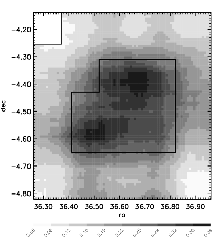
Figure 1: Uneven spectrograph coverage in VVDS-02h field. The grey-scale from the lightest to the darkest grey indicates the sampling rate, with corresponding values shown in the label. The grid used for the colour-code had steps of $30\arcsec$ in Right Ascension and Declination, and for each grid position we used squares of size $7\arcmin$ to estimate the sampling rate. The central area covered by 4 VIMOS passes is highlighted by a solid line.

VVDS-02h field first epoch sample probes a comoving volume (up to  z =1.5) of nearly $1.5\times 10^{6}$ $h^{-3}$Mpc³ in a standard $\Lambda$CDM cosmology. This volume has transversal dimensions $\sim$ 37$\times$37 $h^{-1}$Mpc at  z =1.5 and extends over 3060 $h^{-1}$Mpc in radial direction.

The collected sample contains 6615 galaxies and AGNs with secure redshifts, i.e. redshift determined with a quality flag=2,3,4,9 (6058 with $0.2\leq z\leq 1.5$). We refer the reader to Le Fèvre et al. (2005) for further details about redshift quality flags. Here we only emphasize that, comparing spectroscopic redshifts of objects observed twice by means of independent observations, we conclude that redshifts with flag=2(/3/4) are correctly estimated with a likelihood of 81(/97/$>99$)%. We assigned a flag=9 when in the spectrum there is only a single secure spectral feature in emission. Given the spectral range covered by observations and the flux limits of the survey, this emission line is typically [OII]3727Å  or H$\alpha$ (in very rare cases Ly$\alpha$). Thus flag=9 redshifts have a probability of being correct of $\sim 50$%, being based on the choice between the two most probable emission lines. We double-check the robustness of the likelihood assigned to flag=2 and flag=9 objects, by contrasting spectroscopic estimates against photometric determinations. Photometric redshifts were computed as described in Ilbert et al. (2006), but now using the more recent T0005 release of CFHTLS data ($u^{*}$, g’, r’, i’, z’ filters) and the latest data available from WIRCAM (J, H and K filters, Bielby et al. in preparation). According to this comparison, flag=2(/9) redshifts are correctly inferred with a likelihood of 78(/59)%, a figure which is in good agreement with the independent determination discussed above.

Note, also, that the conclusions of our work are unaffected by the fact of including or not in our analysis flag=9 low quality redshifts. As a matter of fact these objects constitute a small fraction ($<3$%) of the whole sample. Moreover, the effect of possible biases induced by wrong redshift estimates are weakened by the very existence of the galaxy correlation on small scales: if a galaxy with flag=2 is located nearby (on the sky) to other galaxies with similar (but more secure) redshift, the likelihood that it shares the same redshift actually increases with respect to the probability determined on the basis of our analysis.

2.2 Mock catalogues

We made extensive use of mock catalogues, both to test the potential for group searches of the VVDS-02h field data and to tune the parameters of the group-finding algorithm for optimal detection.

Before introducing any particular group-finding algorithm, one needs to test which limits in group reconstruction are imposed by the specific characteristics of the VVDS survey design. With mock catalogues mimicking VVDS-02h field we were able to explore which groups are lost irretrievably due to the survey sparse galaxy sampling. Furthermore we were able to assess how our measurement of the line of sight velocity dispersion of group galaxies is degraded by both the sampling rate and the non negligible VVDS redshift measurement error. After having explored these limits, we then moved to test and optimize the group-finding algorithm, within the ranges in redshift and velocity dispersion where we found that VVDS-02h data allow a reliable group reconstruction.

Mock catalogues were obtained by applying the semi-analytic prescriptions of De Lucia & Blaizot (2007) to the dark matter halo merging trees extracted from the Millennium Simulation (Springel et al., 2005). The simulation contains $N=2160^{3}$ particles of mass $8.6\times 10^{8}h^{-1}M_{\odot}$ within a comoving box of size 500 $h^{-1}$Mpc on a side. The cosmological model is a $\Lambda CDM$ model with $\Omega_{m}=0.25$, $\Omega_{b}=0.045$, $h=0.73$, $\Omega_{\Lambda}=0.75$, $n=1$ and $\sigma_{8}=0.9$. The positions and velocities of all simulated particles were stored at 63 snapshots, spaced approximately logarithmically from $z=20$ to the present day. Dark matter halos are identified using a standard friends-of-friends (FOF) algorithm with a linking length of 0.2 in units of the mean particle separation.

In this simulation, group galaxies are those in the same FOF halo, identified with a unique ID. For each simulated group a wealth of physical information are available: galaxy membership, virial mass (computed directly using the simulated particles), virial radius and virial velocity dispersion (both computed from the virial mass, through scaling laws and the virial theorem). The virial mass is computed within the radius where the halo has an overdensity 200 times the critical density of the simulation.

It is worth noticing that the model used to construct light-cones from the MILLENNIUM simulation has been shown to be quite successful in reproducing several basic properties of our real data set. The most important are the average redshift distribution $n(z)$ (Meneux et al., 2008) and the global Luminosity Function LF (Zucca et al., in preparation), that are in good agreement with the real VVDS-02h $n(z)$ and LF, with the only exception of a slight excess of galaxies in the $n(z)$ mock samples for $z<0.5$. It should be noticed that such a small difference in $n(z)$ does not affect the completeness and purity values (see Section 5.1) of our group catalogue, as we specifically tested using separately the mocks with the most similar and the most different $n(z)$. Moreover, in Meneux et al. (2008) it is shown that the galaxy clustering in the MILLENNIUM simulation light cones is consistent with the one measured using the VVDS-02h sample.

Through the Database built for the Millennium Simulation (Lemson & Virgo Consortium, 2006), we selected 10 $(1\times 1)$ deg² independent MILLENNIUM light cones (generated with the code MoMaF, Blaizot et al., 2005), from which we extracted several kinds of mocks, according to our purposes. First of all, we extracted $(1\times 1)$ deg² flux limited samples, with the same flux limits as VVDS-02h sample ($17.5\leq I_{AB}\leq 24$). These catalogues have 100% sampling rate, and no redshift measurement error added. We called these catalogues $M(100,0)$, the first number in brackets indicating the sampling rate and the second the redshift error. Then we randomly depopulated these catalogues to obtain subsets with 33%, 17% and 10% sampling rate, mimicking roughly the sampling rate of the 4 passes, 2 passes and 1 pass areas of the VVDS-02h field. These catalogues are called $M(33,0)$, $M(17,0)$ and $M(10,0)$ respectively. With these mock catalogues and taking advantage of the known group membership we were able to assess how much a group catalogue is depopulated when sampling rate is lowered to values typical of those of VVDS-02h field.

As a further step, we added redshift measurement errors to the 33% sampling rate mocks, randomly chosen from a Gaussian distribution centered on 0 with $\sigma=275$ km/s. This way we take into account the mean redshift measurement error of our real data. We called these mock catalogues $M(33,275)$. With these mock catalogues, we were able to test how well we can determine group virial velocity dispersion when the survey has flux limits, sampling rate and redshift measurement errors mimicking those of the 4 passes areas of the VVDS-02h field.

As a last step we needed mock catalogues to test how effective is the group-finding algorithm we adopted in identifying those groups surviving in a sample like the VVDS-02h one. To test the efficiency of our algorithm we used 20 “VVDS-like” mocks extracted from MILLENNIUM simulation. These mocks have the same flux limits, geometry, uneven sampling rate, redshift error measurement as the VVDS-02h sample (see Pollo et al., 2005 and Meneux et al., 2008 for the preparation of these mocks). Subtler effects, like those introduced by slit positioning bias, have also been included, as the same slit positioning tool used for VVDS-02h sample has been used, with the same optimization criteria, to generate the VVDS-like mocks. Moreover, the areas masked in the real photometric catalogue because of bright stars and because of a beam of scattered light have also been masked in the VVDS-like mocks.

For the sake of clarity, we emphasize that whenever we refer to the ‘FOF’ or ‘simulated’ groups in all the above-mentioned mock catalogues, we mean the sets of galaxies within the same original FOF halo provided by the simulation itself, before any depopulating process: we never ran any FOF algorithm on mocks after extracting $M(100,0)$, $M(33,0)$, $M(17,0)$ and $M(10,0)$, $M(33,275)$ and “VVDS-like” mocks from simulations.

3 Preliminary tests

3.1 Testing the effects of VVDS survey strategy on groups

In this section we explore how well the group catalogue extracted from a VVDS-like survey trace the group population of an ideal survey which is purely flux-limited. In a real flux limited galaxy survey with a sampling rate lower than $100$%, most groups will have a smaller number of members and some will even go undetected. We want to assess the fraction of groups that “survive” as such (i.e. with at least 2 members) in a survey with a sampling rate like the one in VVDS-02h. To identify groups, both in the full flux limited and in the various ‘observed’ catalogues, we used at this phase the identification number of FOF groups in the Millennium database. In other words, we consider only the limitations introduced by the survey strategy, neglecting for the moment further complications introduced by the incompleteness/failures of the specific group finding algorithm we used.

In Figure 2 we plot the fraction of groups in mock catalogues flux limited at $17.5\leq I_{AB}\leq 24.0$ that survived after applying a sampling rate corresponding to 1/2/4 passes regions (i.e. 10%, 17% and 33% respectively) as indicated by different lines. Practically, we plot the ratio between the number of groups in $M(10,0)$, $M(17,0)$ and $M(33,0)$ catalogues and the number of groups in $M(100,0)$ catalogues. This ratio has been computed in not-independent running redshift bins of $\Delta z=0.3$: continuous lines are fits along all the bins, while for reference the ratios corresponding to the $M(33,0)$ catalogues are also shown for each redshift bin as red diamonds. Note that the number of groups with $\sigma_{vir}\geq 650$ km/s is quite low, mainly because of the small field of view, thus the fraction of survived groups at $z\leq 0.8$ fluctuates around a mean value that we use to fit a straight line. These fluctuations, however, only in the worst cases are as high as 10%. This is also true for $M(10,0)$ and $M(17,0)$ catalogues, for which we do not plot single points not to crowd the figure. The horizontal dashed line at a fraction value equal to 50% is shown for reference. The three panels correspond to different cuts in the virial line of sight velocity dispersion ($\sigma_{vir}$) quoted in the mocks, as indicated by the label (from now onwards all velocity dispersions quoted will be line of sight velocity dispersions).

Figure 2 shows that in 2 and 4 passes areas we can recover the majority ($\geq 50\%$) of groups down to $\sigma_{vir}\sim 350$ km/s in the full redshift range below $z=1.0$. Obviously going to higher values for $\sigma_{vir}$ allows to extend further the redshift range. Such lower limit for $\sigma_{vir}$ is in agreement with the one imposed by the non negligible redshift measurement error of VVDS survey. As we will see in the next paragraph, for groups with $\sigma_{vir}\leq 350$ km/s our measurements of velocity dispersion are quite unreliable.

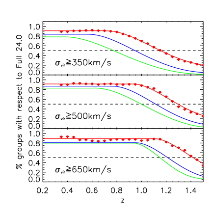
Figure 2: The fraction, as a function of redshift, of “surviving” groups when the sampling rate is decreased from a purely flux limited simulated sample $17.5\leq I_{AB}\leq 24.0$ (i.e. with 100% sampling rate) to $\sim$33% (4 passes area, red line), $\sim$17% (2 passes, blue line) and $\sim$10% (1 pass area, green line). The fraction has been computed in not-independent running redshift bins of $\Delta z=0.3$: continuous lines are fits along all the bins, while for reference the fractions corresponding to the $M(33,0)$ catalogues are also shown for each redshift bin as red diamonds. Different panels show different cuts in $\sigma_{vir}$, as quoted in each panel. The horizontal dashed line at a fraction value equal to 50% is for reference.

3.2 Estimating group virial l.o.s. velocity dispersion

A robust determination of the line-of-sight velocity dispersion of galaxies in group is essential if we are to infer the group mass in a reliable way. When group members are sparsely sampled, as it is the case for VVDS-02h data, the “gapper method”, originally suggested by Beers et al. (1990), has proved to be the most robust velocity dispersion estimator (see also Girardi et al., 1993). This method measures velocity dispersion exploiting the velocity gaps in the given velocity distribution of galaxies, using the following formula:

$$\sigma_{G}=\frac{\sqrt{(}\pi)}{N(N-1)}\sum_{i=1}^{N-1}i(N-i)(v_{i+1}-v_{i})$$ (1)

where the line of sight velocities $v_{i}$ are sorted into ascending order. Beers et al. (1990) show in their Table II that this method reliably estimates the velocity dispersion with an efficiency $>90$% for groups with $\sim 5-10$ elements, thanks to its robustness in recovering the dispersion of a distribution also in the more general case of a contaminated Gaussian distribution. It is important to emphasize that this range of group members is well suited for the study we present in this work. On the one hand, we consider the velocity dispersion reliably measurable only for groups with at least 5 members, and on the other hand the large majority of groups surviving in “VVDS-like” mocks have $\leq 10$ members.

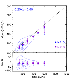
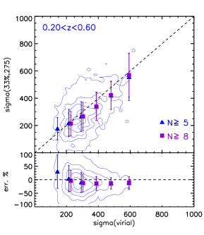
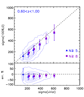
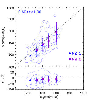
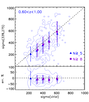
Figure 3: Comparison of line of sight velocity dispersion $\sigma_{meas}$ computed in $M(100,0)$, $M(33,0)$ and $M(33,275)$ mocks ($1^{st}$, $2^{nd}$ and $3^{rd}$ column respectively) with the virial velocity dispersion $\sigma_{vir}$. The first row is for the redshift bin $0.2<z<0.6$, and the second for $0.6<z<1.0$. In each plot, the upper panel shows isodensity contours in the plane $\sigma_{meas}$ versus $\sigma_{vir}$ for groups with at least 5 members. Blue triangles are the median (on $x$ axis) and mean (on $y$ axis) values of single points grouped in bins of $\sigma_{vir}$, with vertical error bars being the rms of mean values. The bins on the $x$ axis have the following limits: 0.5 - 150 - 250 - 350 - 450 - 550 - 1100 km/s. Purple squares are the same as triangles but for groups with at least 8 members. The lower panel in each plot shows the percentage error (with its rms) when we compare $\sigma_{meas}$ and $\sigma_{vir}$. Triangles and squares are plotted only when the corresponding $\sigma_{vir}$ bin contains at least 15 objects. See text for further details.

Hereafter, when discussing “measured” velocity dispersions ($\sigma_{meas}$) we will refer to velocity dispersions obtained applying the gapper method to the members of the given group. Of course, we corrected this velocity dispersion taking into account the scaling between redshift and velocity. Thus we used:

$$\sigma_{meas}=\frac{\sigma_{G}}{1+z}$$ (2)

where $z$ is the redshift of the group.

In this section we want to test whether our measurement of the line of sight velocity dispersion $\sigma_{meas}$ is a reliable estimate of the virial velocity dispersion $\sigma_{vir}$ (as listed in the mock catalogues). For this comparison we used $M(100,0)$, $M(33,0)$ and $M(33,275)$. We called the $\sigma_{meas}$ of these three kinds of catalogues $\sigma(100,0)$, $\sigma(33,0)$ and $\sigma(33,275)$ respectively. In the case of a non-zero redshift measurement error, such as in $M(33,275)$ mock catalogues, we took the error itself into account when computing $\sigma_{meas}$, so that the error ($v_{err}$) was subtracted in quadrature as follows:

$$\sigma(33,275)^{2}=\frac{max[0,\sigma(33,275)_{G}^{2}-v_{err}^{2}]}{(1+z)^{2}}$$ (3)

where $\sigma(33,275)_{G}$ is the velocity dispersion measured in $M(33,275)$ mocks with Equation 1, $v_{err}=275$ km/s and $z$ is the redshift of the group. When $\sigma(33,275)=0$ we considered the velocity dispersion not measurable given the redshift error.

Figure 3 shows the comparison of $\sigma_{vir}$ with $\sigma(100,0)$, $\sigma(33,0)$ and $\sigma(33,275)$, respectively in the first, second and third column. The first row is for the redshift bin $0.2<z<0.6$, and the second for $0.6<z<1.0$. In each plot, the upper panel shows isodensity contours in the plane $\sigma_{meas}$ versus $\sigma_{vir}$ for groups with at least 5 members. Blue triangles are the median (on $x$ axis) and mean (on $y$ axis) values of single points grouped in bins of $\sigma_{vir}$, with vertical error bars being the rms of mean values. As a reference, purple squares are the same as triangles but for groups with at least 8 members. The lower panel in each plot shows the systematic offset of the relation in the upper panel; the offset is expressed as a percentage error (with its rms) computed as follows:

$$err.\%=\frac{[\sigma_{meas}-\sigma_{vir}]}{\sigma_{vir}}\times 100,$$ (4)

where $\sigma_{meas}$ is $\sigma(100,0)$, $\sigma(33,0)$ and $\sigma(33,275)$ in the three columns respectively. Symbols have the same meaning as in the upper panel.

Results graphically shown in Fig. 3 can be summarized as follows:

• Effects due to the VVDS-02h flux limit. The plots in the first column show that even in the ideal case of purely flux limited mock catalogues with 100% sampling rate and without redshift measurement error, the measured velocity dispersion $\sigma(100,0)$ systematically underestimates $\sigma_{vir}$. This systematic offset, shown in the lower part of the plots, is always below 20%, with a smaller scatter for increasing $\sigma_{vir}$ and for the lower redshift bin. Such an offset can easily be understood by noticing that in a flux limited survey, even with a 100% sampling rate, moving to higher redshifts groups will progressively lose the fainter members that lie outside the selected flux range. As a consequence the measured velocity dispersion underestimates the real virial velocity dispersion, as the “surviving” galaxies are the brighter, usually found in group cores.

• Effects due to the lower sampling rate introduced by VVDS-02h strategy. The plots in the second column show that if we decrease the sampling rate from 100% to 33%, our ability in recovering $\sigma_{vir}$ decreases as well, as expected. The systematic offset is not significantly worse than in mocks with 100% sampling rate, but the scatter around the systematic offset is larger, especially for low $\sigma_{vir}$.

• Effects due to VVDS redshift measurement error. Finally, the plots of the third column illustrate the fact that when we add 275 km/s of redshift error, low $\sigma_{vir}$ are very difficult to recover, while, for $\sigma_{vir}>350$ km/s, the systematic offset and its rms remain below 25% with a slightly higher scatter for the higher redshift bin.

Figure 3 convincingly demonstrates that the estimate of the velocity dispersion is robust only in groups with $\sigma_{vir}>350$ km/s. It also serves the following purpose: it forecasts the precision with which the measured velocity dispersion traces a specific $\sigma_{vir}$ of the matter particles in the halo once the VVDS sampling rate and spectroscopic uncertainties are taken into account. As a matter of fact, when we analyze the real VVDS-02h group catalogue, only the estimate $\sigma_{meas}$ are available, and nothing is known about $\sigma_{vir}$. We should therefore ask also the reverse question of how far a given value of $\sigma_{vir}$ is from the observed $\sigma_{meas}$. This means that we have to take $\sigma_{meas}$ as reference when we compute the percentage error. We show the results of this analysis in Figure 4 in which, for any given bin of $\sigma(33,275)$ we plotted the mean systematic offset from the real underlying $\sigma_{vir}$, computed as a percentage error on $\sigma(33,275)$ as follows:

$$err.\%=\frac{[\sigma(33,275)-\sigma_{vir}]}{\sigma(33,275)}\times 100.$$ (5)

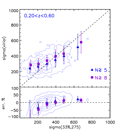
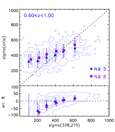
Figure 4: As the plots in the last column of Figure 3, but with exchanged axes. In this case the binning is made according to $\sigma(33,275)$ and not $\sigma_{vir}$.

Also in this case, when considering $\sigma(33,275)$ greater than 350 km/s we are able to recover $\sigma_{vir}$ with an error of $<30$% and $<20$% for groups with $N\geq 5$ and $N\geq 8$ respectively. Therefore, for velocity dispersions above 350 km/s and despite the relatively large error in redshift measurements causes a systematic increase in the estimated $\sigma(33,275)$, we can still reconstruct a sensible value of $\sigma_{vir}$ in the VVDS-2h 4 passes region. We carried on a similar check for groups in 1 pass and 2 passes regions, and verified that results are qualitatively similar to those obtained in the 4 passes area.

Globally, our analysis suggests that we can use VVDS-02h data as a suitable sample for extracting high-$z$ groups.

4 The group-finding algorithm

Several geometrical algorithms have been proposed to identify groups and clusters from the 3-dimensional distribution of galaxies, that is by optically identifying them within spectroscopic redshift survey (see Section 1).

In this work we identified groups using the Voronoi-Delaunay Method (Marinoni et al., 2002). In short, the VDM combines information from the three-dimensional Voronoi diagram and its dual, the Delaunay triangulation. The Voronoi diagram (Voronoi, 1908) is a polyhedral partition of 3D space, each polyhedron surrounding a galaxy and defining the unique volume containing all the points that are closer to that galaxy than to any other galaxy in the sample. The Delaunay complex (Delaunay, 1934) also contains proximity information. It is defined by the tetrahedra whose vertices are sets of four galaxies, that have the property that the unique sphere that circumscribe them does not contain any other galaxy. The center of the sphere is a vertex of a Voronoi polyhedron, and each face of a Voronoi polyhedron is the bisector plane of one of the segments that link galaxies according to the Delaunay complex.

The basics of the VDM code is as follows. The denser the environment in which a galaxy live, the smaller the Voronoi volume which is associated to it. Therefore the Voronoi partition allows for an immediate identification of the central regions of structures. Complementarily, the Delaunay triangulation assigns galaxy members to the identified core. Note that a crucial difference between the VDM and other methods is that, since it preliminarily identifies group centers, group membership reconstruction proceed radially outward, from the densest cores towards the outskirts of the structures.

An advantage offered by the Voronoi-Delaunay method is that it exploits the natural clustering of the galaxies in the sample. For example the dimension of the volume assigned to each galaxy locally depends on the number density of the objects surrounding the galaxy itself. It is thus adaptively and unparametrically rescaled and not predefined on the basis of some fixed length parameter. Moreover, galaxies that are Delaunay connected to the central cores are processed with cylindrical windows whose dimensions are locally scaled on the basis of physical relations observed in simulated (and real) samples of groups and clusters. The specific set of VDM parameters is thus designed in such a way to offer the maximum of flexibility in selecting groups according to the a-priori physical information we have on their structure. As a consequence, a fine-tuned VDM algorithm has been proven to be very efficient in reconstructing intrinsic characteristics of groups, such as for example the line of sight velocity dispersion of their members (Marinoni et al., 2002).

The Voronoi-Delaunay method was specifically designed to avoid some known drawbacks characterizing standard group-finding algorithms such as for example the FOF and the hierarchical methods. These methods are based on user-specified parameters (the FOF linking length, the ‘affinity’ threshold in the hierarchical method) that do not depend on the real distribution of galaxies. One of the negative consequences is that spatially closed but unrelated structures are often merged together in a single system. Moreover, some dynamical properties of clusters are very sensitive to the adopted group-finding algorithm: for example, the velocity dispersion of groups identified by the FOF algorithm is found to be systematically higher (by nearly $30$%) than that of groups found by the hierarchical algorithm, even when both algorithms are optimized on the same galaxy sample (Giuricin et al., 2001).

We will now briefly summarize how the VDM works, although detailed descriptions can be found in Marinoni et al. (2002) and also in Gerke et al. (2005) (from which we adopted some technical improvements).

At first, the algorithm computes the Voronoi-Delaunay mesh following the prescriptions in Barber et al. (1996) and Mirtich (1996). It then searches for groups with a 3-step procedure. At each step, new group members are identified by means of a cylindrical window (of radius $R$ and half-length $L$) which is used to scan Delaunay connected galaxies and to decide whether or not they are cluster members. Phase I concerns the 3-D identification of group seeds. In Phase II the algorithm determines group central richness, and finally in Phase III an adaptive scaling based on N-$\sigma$ relation is used to rescale cylinder dimensions depending on group richness found in Phase II. A detailed explanation of each of these three steps follows in sections 4.1, 4.2 and 4.3.

The radius and the half-length of the cylinders of Phase I ($\mathcal{R}_{I}$ and $\mathcal{L}_{I}$) and of Phase II ($\mathcal{R}_{II}$ and $\mathcal{L}_{II}$), together with $r$ and $l$, the scaling factor used to determine respectively the radius and the half-length of the cylinder of Phase III ($\mathcal{R}_{III}$ and $\mathcal{L}_{III}$), are free parameters of the algorithm. They have to be optimized using physical information about clusters.

The choice of a cylindrical shape for the search window is physically motivated by the fact that the gravitational field of galaxy overdensities induces peculiar velocities whose effect is to make the galaxy distribution to appear elongated in the redshift direction. The only way to take this into account is by using a search window with a radial extension much longer than the transversal dimension, in order not to miss group members. Note that we use a cylindrical window also in Phase I, while in Marinoni et al. (2002) Phase I search window had a spherical shape. The original choice of a spherical window for the first phase was physically motivated by the fact that galaxies residing in the highest density peaks, i.e. the central cores of groups and clusters, are expected to have smaller peculiar velocities. However, we verified that for less rich systems, i.e. loose groups as those we expect to recover in the VVDS sample, the best choice is a cylindrical window. In particular, the survey quite large redshift measurement error together with the sparse sampling rate motivate our new choice.

As we want the length of search cylinders to correspond roughly to the peculiar velocity of the galaxies in the group, we have to consider that the mapping between redshift interval and peculiar velocity changes with redshift, and thus, following Gerke et al. (2005), our algorithm automatically rescales cylinder lengths $\mathcal{L}(z)$ as a function of $z$, using the equation:

$$\mathcal{L}(z)=[s(z)/s(z_{0})]\mathcal{L}(z_{0}),$$ (6)

where $z_{0}$ is a reference redshift (see Section 4.2 for details) and

$$s(z)=\frac{1+z}{\sqrt{\Omega_{M}(1+z)^{3}+\Omega_{\Lambda}}}.$$ (7)

This scaling as a function of redshift is applied to all $\mathcal{L}_{I}$, $\mathcal{L}_{II}$ and $\mathcal{L}_{III}$.

4.1 Phase I.

In Phase I galaxies are at first ranked according to the increasing size of their Voronoi volume. A cylinder with radius $\mathcal{R}_{I}$ and half length $\mathcal{L}_{I}$ is then centered on the galaxy with smallest Voronoi volume. All galaxies inside the cylinder and Delaunay-connected with the central galaxy are considered group members and called first-order Delaunay neighbours. The central galaxy and its first-order Delaunay neighbours are considered a group seed. In the case there are no other galaxies in the cylinder, the central galaxy is rejected as potential seed. Thus, the choice of $\mathcal{R}_{I}$ and $\mathcal{L}_{I}$ determines the final number of identified groups. At the end of this Phase the barycenter of the seed is computed, using the positions of the central galaxy and its first-order Delaunay neighbours.

Then the algorithm processes the full sequence of Phases for the found seed. After Phase II and Phase III are completed, the whole procedure is reiterated by selecting from the sorted list the first galaxy not yet assigned to a group.

4.2 Phase II.

In the second phase a different cylindrical window with radius $\mathcal{R}_{II}$ and half length $\mathcal{L}_{II}$ is centered on the barycenter determined in Phase I, and it is used to determine the central richness of the group. All galaxies that fall in the Phase II cylinder and are connected to the first-order Delaunay neighbours are called second-order Delaunay neighbours, and are considered further group members. The total number of group members after this phase (the central galaxy plus first- and second-order neighbours) is considered as the central richness $N_{II}$ of the group.

A reliable estimate of $N_{II}$ is important as it controls the adaptive search window used in Phase III (see below). From one hand, the fact of considering only Delaunay-connected galaxies minimizes the inclusion of interlopers in $N_{II}$. On the other hand, in a flux limited survey like VVDS, the $N_{II}$ distribution varies as a function of redshift, because of the variation of the luminosity limit with redshift. To ensure a uniform group population, $N_{II}$ has to be corrected as a function of $z$:

$$N_{II}^{corr}(z)=N_{II}\frac{\langle\nu(z_{0})\rangle}{\langle\nu(z)\rangle}$$ (8)

Here $z_{0}$ is the redshift zero-point considered as reference, and $\langle\nu(z)\rangle$ is the comoving number density, that we calculated by smoothing the redshift distribution of the galaxy sample, and then dividing it by the differential comoving volume element at the considered redshift. In Gerke et al. (2005), $z_{0}$ is the lower limit of the DEEP2 galaxy redshift distribution $n(z)$, i.e. $z_{0}=0.7$. In the case of VVDS-02h sample, the lower limit in $n(z)$ is $z=0.2$, but at this redshift the volume covered by the VVDS-02h is small. Because of this, $\langle\nu(z=0.2)\rangle$ can be poorly constrained. Moreover, $\langle\nu(z)\rangle$ decreases very rapidly from $z=0.2$ up to $z=1.0$. Thus we chose $z_{0}=0.7$ as a compromise between high statistics (it is roughly the peak of our $n(z)$ distribution) and not yet so large survey volume.

At the end of Phase II the barycenter position is readjusted using all $N_{II}$ members.

4.3 Phase III.

Finally, in Phase III the algorithm reconstructs the full set of group members, using a new search window which is centered on the group barycenter determined at the end of Phase II and with dimensions determined according to the following basic scaling relations.

Assuming that groups are singular isothermal spheres, at any given distance $r$ from the center the mass density distribution is related to the velocity dispersion through the equation $\rho(r)=\sigma^{2}/(2\pi Gr^{2})$ (Binney & Tremaine, 1988). Since $M(r)=4\pi r^{3}\rho(r)/3$, and by defining $r_{vir}$ as the radius of a spherical volume within which the mean density is $\Delta_{c}$ times the critical density at the considered redshift, we find that $M_{vir}\propto\sigma^{3}$, where $M_{vir}=M(r_{vir})$ is the virial mass. The virial theorem implies that $M_{vir}\propto\sigma^{3}\propto R^{3}$. therefore, exploiting the correlation between velocity dispersion and central richness, which has been confirmed from loose groups up to massive clusters (for example, see Bahcall, 1981), we end up with the following chain of relations $N_{II}^{corr}\propto M_{vir}\propto\sigma^{3}\propto R^{3}$.

Accordingly, we let the central richness $N_{II}^{corr}$ of each group to control both the radius and the length of the cylindrical search window:

• $\mathcal{R}_{III}=r(N_{II}^{corr})^{1/3}$;

• $\mathcal{L}_{III}=l(N_{II}^{corr})^{1/3}$.

Here, $r$ and $l$ are normalization parameters to be optimized using simulations. Note that the adaptive search window of Phase III will differ from group to group and that all galaxies enclosed within the cylinder are considered as further group members, irrespectively of the order of their Delaunay connections. From now on, we will call richness $N$ the final number of members assigned to each group at the end of Phase III.

5 Optimizing the group-finding algorithm

5.1 Success criteria

In this section we detail the optimization strategy devised to reconstruct groups in the most reliable and unbiased way. To this purpose, we used VVDS-like mock catalogues. We applied the VDM algorithm to them, and compared the groups found by the algorithm with the groups present in the mocks identified by the same FOF identification number (see Subsection 2.2). From now on, we will refer to the FOF groups in the mocks as “fiducial” groups, while groups reconstructed by our algorithm will be called “reconstructed” groups, or simply “VDM” groups.

There are two levels of success we are interested in: 1) success in finding groups, i.e. to establish the level of contamination by interlopers and fake groups, the percentage of missed galaxies and missed groups and other statistics of this kind; 2) success in reproducing group properties, i.e. to accurately measure group properties on a group-by-group basis, and also to reproduce their statistical distribution as accurately as possible.

To test VDM algorithm success in finding the fiducial groups present in the VVDS-like mocks, we used the following quality estimators (see also Marinoni et al., 2002 and Gerke et al., 2005 for more details):

• galaxy success rate $S_{gal}$: fraction of galaxies belonging to fiducial groups that are identified members of reconstructed groups;

• interlopers fraction $f_{I}$: fraction of galaxies identified by the algorithm as members of reconstructed groups but that are interlopers;

• completeness $C$: fraction of fiducial groups that are “successfully” identified in the reconstructed catalogue;

• purity $P$: fraction of reconstructed groups that “correspond” to fiducial groups.

Hence, we now need a quantitative measure to determine whether a fiducial group is detected “successfully” and whether a reconstructed group “corresponds” to a fiducial one. To this purpose, we consider a detection to be successful when more than half of a fiducial group members are detected in the same VDM group. On the contrary, a VDM group corresponds to a fiducial one when more than half of its members belongs to that fiducial group. In general, these two conditions can be verified independently. These general cases are called one-way matches from one group catalogue to the other (from fiducial to VDM or in the opposite direction). But when these conditions are verified simultaneously involving the same fiducial and VDM group in both directions, we have a two-ways match. So we can have a one-way completeness ($C_{1}$) and a one-way purity ($P_{1}$) when we consider only one-way matches in the fiducial and in the reconstructed group catalogue respectively, but also a two-way completeness ($C_{2}$) and a two-way purity ($P_{2}$) can be defined when considering two-ways matches.

On the one hand, knowing absolute value of completeness and purity will help us in optimizing the algorithm, but on the other hand comparing $C_{1}$ with $C_{2}$ and $P_{1}$ with $P_{2}$ we can establish the kind of errors in the reconstructed group catalogue. In fact, when $C_{1}>>C_{2}$, it means that some fiducial groups are one-way successes but not two-ways matches, and thus these fiducial groups contain a low fraction of the members of their reconstructed associated group. This is an indication that VDM algorithm tends to overmerge separated groups in bigger reconstructed groups, or to assign to reconstructed groups too many interlopers. On the other hand, when $P_{1}>>P_{2}$ we know that VDM algorithm is doing the opposite error, i.e. the reconstructed group catalogue is highly fragmented with respect to the fiducial one.

We decided to use these indicators to search for the best set of parameter for our algorithm following some guide lines. The basic idea is to obtain $C_{1}$ and $C_{2}$ as high as possible, while keeping $P_{1}$ and $P_{2}$ at least above 50%. Moreover, we would like not to produce a highly overmerged ($C_{1}>>C_{2}$) or a highly fragmented ($P_{1}>>P_{2}$) catalogue, and therefore we tried to obtain $C_{1}\approx C_{2}$ and $P_{1}\approx P_{2}$.

5.2 Algorithm optimization

We applied the VDM algorithm to 20 VVDS-like mocks, obtaining group catalogues for the full redshift range $0.2\leq z\leq 1.5$, but for the reasons discussed in Section 3.1 we implemented the optimization strategy only in the range $0.2\leq z\leq 1.0$.

With a trial and error approach we explored the flexibility of the 6 VDM parameters in recovering groups in a robust way. We allowed each parameter to vary in a wide range. In particular, 1) we let $\mathcal{R}_{I}$ and $\mathcal{R}_{II}$ increase up to 1 $h^{-1}$Mpc, with no lower limit: this because we wanted the radii to span projected dimensions up to typical central radius of massive clusters (Bahcall, 1981). 2) We let $r$ span the range $0.4\leq r\leq 1.5$, as we want the radius of the last search cylinder to be equal or larger than small groups typical size ($\sim 0.5$ $h^{-1}$Mpc, see Borgani et al., 1997 and references therein) and smaller than an Abell radius ($\sim 1.5$ $h^{-1}$Mpc, see Borgani et al., 1997). 3) We let $\mathcal{L}_{I}$, $\mathcal{L}_{II}$ and $l$ vary from 4 to 20 $h^{-1}$Mpc, to include clusters with velocity dispersion as high as 2000 km/s also at high redshift ($z\sim 1$). In this case the lower limit is mainly suggested by our redshift measurement error, that has to be added to peculiar velocities. We imposed to $\mathcal{R}_{III}$ and $\mathcal{L}_{III}$ the same limits as $r$ and $l$. Nevertheless, we also checked the performances of the algorithm when no limits are applied to $\mathcal{R}_{III}$ and $\mathcal{L}_{III}$, and we verified that, with the exception of very few cases, $\mathcal{R}_{III}$ and $\mathcal{L}_{III}$ ‘behave well’, as we expected as the whole algorithm is based on physical scales and scaling laws.

Exploring the 6D parameter space, we found the parameter set that kept $C_{1}$ and $C_{2}$ as high as possible and $P_{1}$ and $P_{2}$ at least above 50%, while monitoring also the behavior of the group properties, both on a group by group basis and on a statistical point of view. Then we moved slightly around these chosen values with smaller steps, to search for a possible finer tuning.

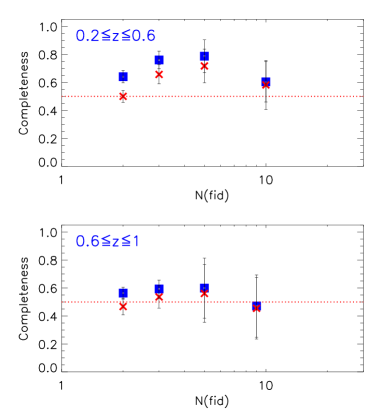
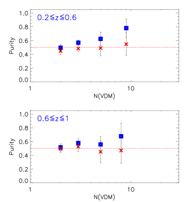
Figure 5: $C_{1}$ and $C_{2}$ statistics as a function of “fiducial” group members (on the left) and $P_{1}$ and $P_{2}$ statistics as a function of “reconstructed” group members (on the right). One-way statistics are shown as blue squares, and two-way statistics are shown as red crosses. C and P have been computed separately in each mock: in these plots points are C and P values averaged over all mocks, while error bars are their $rms$. On the $x$ axis we grouped the number of elements in the following way: [N=2],[N=3,4] ,[N=5,6] and [N$\geq$7]

At the end of this finer search, we found the following parameter set, from now on called the best set of parameters:

- $\mathcal{R}_{I}=0.28$ $h^{-1}$Mpc

- $\mathcal{L}_{I}=7.0$ $h^{-1}$Mpc

- $\mathcal{R}_{II}=0.6$ $h^{-1}$Mpc

- $\mathcal{L}_{II}=5.0$ $h^{-1}$Mpc

- $r=0.55$ $h^{-1}$Mpc

- $l=14.0$ $h^{-1}$Mpc

We assigned to each group a redshift and a position in the R.A.-Dec. plane, respectively defined as the median values of redshift, Right Ascension and Declination of the group members.

Values of the quality parameters $C_{1}$, $C_{2}$, $P_{1}$, $P_{2}$, $S_{gal}$ and $f_{I}$ can be found in Table 1. Note that, to test the quality of the algorithm also as a function of redshift, we considered separately two redshift bins ($0.2\leq z\leq 0.6$ and $0.6\leq z\leq 1.0$).

We analyzed completeness and purity also as a function of group richness. Figure 5 shows $C_{1}$ and $C_{2}$ as a function of “fiducial” group members and $P_{1}$ and $P_{2}$ as a function of “reconstructed” group members. One-way statistics are shown as blue squares, and two-ways statistics are shown as red crosses. C and P have been computed separately in each mock. In Figure 5 we plot C and P values averaged over all mocks, while error bars are their rms. The differences between $C_{1}$ and $C_{2}$ and between $P_{1}$ and $P_{2}$ indicate that our group catalogue will not be completely free neither from overmerging nor from fragmentation. Moreover, Figure 6 shows that, while the galaxy success rate $S_{gal}$ does not vary much as a function of $N$, the interloper fraction $f_{I}$ decreases by a factor of $\sim 2$ from $N\geq 2$ to $N\geq 9$.

Table 1: Quality statistics ($C_{1}$, $C_{2}$, $P_{1}$, $P_{2}$, $S_{gal}$ and $f_{I}$, see text for details) of the reconstructed group catalogue, for two different redshift bins and for the whole redshift range. The first table shows $C_{1}$, $C_{2}$, $P_{1}$, $P_{2}$, $S_{gal}$ and $f_{I}$ for all groups, while the second table for groups with at least 3 members. Each parameter is computed as the mean over the 20 VVDS-like mocks, and the associated error is its $rms$.

Quality statistics for N$\geq$2
Quality parameter	$0.2\leq z\leq 0.6$	$0.6\leq z\leq 1.0$	$0.2\leq z\leq 1.0$
$C_{1}$	$0.68\pm 0.03$	$0.57\pm 0.04$	$0.63\pm 0.03$
$C_{2}$	$0.56\pm 0.04$	$0.49\pm 0.05$	$0.53\pm 0.03$
$P_{1}$	$0.56\pm 0.02$	$0.55\pm 0.04$	$0.56\pm 0.02$
$P_{2}$	$0.48\pm 0.04$	$0.50\pm 0.04$	$0.49\pm 0.03$
$S_{gal}$	$0.72\pm 0.03$	$0.59\pm 0.03$	$0.67\pm 0.02$
$f_{I}$	$0.38\pm 0.02$	$0.43\pm 0.04$	$0.40\pm 0.02$

Quality statistics for N$\geq$3
Quality parameter	$0.2\leq z\leq 0.6$	$0.6\leq z\leq 1.0$	$0.2\leq z\leq 1.0$
$C_{1}$	$0.73\pm 0.06$	$0.57\pm 0.05$	$0.67\pm 0.04$
$C_{2}$	$0.65\pm 0.06$	$0.52\pm 0.06$	$0.60\pm 0.03$
$P_{1}$	$0.61\pm 0.03$	$0.58\pm 0.05$	$0.60\pm 0.03$
$P_{2}$	$0.50\pm 0.05$	$0.51\pm 0.07$	$0.50\pm 0.05$
$S_{gal}$	$0.75\pm 0.04$	$0.60\pm 0.04$	$0.70\pm 0.03$
$f_{I}$	$0.35\pm 0.03$	$0.40\pm 0.05$	$0.37\pm 0.02$

Figure 6: Interlopers fraction $f_{I}$ (empty symbols) and galaxy success rate $S_{gal}$ (full symbols) for different lower limits of group richness ($x$ axis). Diamonds are for the redshift bin $0.2\leq z\leq 0.6$, triangles for $0.6\leq z\leq 1.0$ and squares for the entire range $0.2\leq z\leq 1.0$. $S_{gal}$ and $f_{I}$ have been computed separately in each mock. In this plot, points are $S_{gal}$ and $f_{I}$ values averaged over all mocks, while error bars are their $rms$.

5.3 Tests on recovered group properties

The n(z) distribution. We analyzed how well the “fiducial” group distribution $n_{fid}(z)$ as a function of redshift is recovered by the distribution $n_{VDM}(z)$ of the groups found by the algorithm. We averaged the $n_{fid}(z)$ distribution over 20 independent VVDS-like mocks to obtain its mean value, plotted as a continuous line in Figure 7. In the Figure, the mean $n_{VDM}(z)$ for the same 20 independent mocks is shown as black points, with vertical bars being the rms among the 20 mocks. The plot shows that the difference between $n_{VDM}(z)$ and $n_{fid}(z)$, despite the presence of fake and/or missing groups in the VDM catalogue, is within the errors. A $\chi^{2}$ test between the two mean distributions gives $\chi^{2}=1.4$. We therefore conclude that the two $n(z)$ distributions are statistically consistent with each other, even if there is a tendency for having more VDM reconstructed groups at low redshift. We repeated the same test using only groups with at least 5 members and with $\sigma\geq 350$ km/s, that is those groups for which we are sure we can compute a reliable velocity dispersion, and we found also in this case that $n_{VDM}(z)$ and $n_{fid}(z)$ are consistent with each other.

Velocity dispersion. As discussed above, the comparison between group properties in the fiducial and in the reconstructed catalogue is an important check to verify that VDM algorithm is not only able to recover real groups, but also to preserve their characteristics. This means that when we compare the two catalogues on a group-by-group basis, the fractions of interlopers and missing galaxies modify group properties only below some tolerance level. The same has to hold also for the fiducial and reconstructed statistical distributions of these properties, when considering that the reconstructed catalogue contains fake groups and it misses some groups.

For each VDM group, we measured the velocity dispersion $\sigma_{VDM}$ of its galaxies using Equation 1, correcting it as in Equation 3. Figure 8 shows the comparison between the velocity dispersion in the reconstructed groups ($\sigma_{VDM}$) and the virial velocity dispersion ($\sigma_{vir}$ quoted in the simulations) of the fiducial groups in VVDS-like mocks on a group-by-group basis. Only two-ways matches are considered. The Figure is divided in two panels as Figure 4: the upper part shows the scatter plot, the lower shows the percentage error, computed as in Figure 4. Green and blue triangles are groups with at least 5 members, orange and purple squares groups with at least 8 members; green and orange points are single groups, while blue and purple symbols are the median (on $x$ axis) and mean (on $y$ axis) values in bins of the property on the $x$ axis. Vertical error bars are rms of mean values.

This scatter plot shows the following: on a group-by-group basis, for $\sigma_{VDM}\geq 350$ km/s, close to the intrinsic limit set by the flux-limited nature of the VVDS catalogue, the correlation between $\sigma_{VDM}$ and $\sigma_{vir}$ is such that $\sigma_{VDM}$ overestimates $\sigma_{vir}$, but on average always by $\lesssim 30$% for groups with at least 5 members, while this overestimate is on average $\lesssim 10$% for groups with at least 8 members. In fact, we have shown in Section 3.2 that the velocity dispersion $\sigma_{meas}$ that one can measure in groups within a VVDS-like data sample is not a reliable estimator of $\sigma_{vir}$ for $\sigma_{meas}\leq 350$ km/s.

Besides the group-by-group comparison, it is also interesting the analysis of the velocity dispersion distributions, thus including unrecovered and fake groups in the fiducial and in the reconstructed catalogues respectively. Figure 9 shows the comparison between $n(\sigma_{vir})$ and $n(\sigma_{VDM})$ distributions (the solid line and the black diamonds respectively). Values on the $y$ axis are averaged over 20 VVDS-like mocks. Vertical bars associated to $\sigma_{VDM}$ points are their rms over the 20 mocks. One can notice that the area below the two distributions is different. This mainly because in $\sigma_{VDM}$ distribution we excluded groups for which we were not able to measure $\sigma$, i.e. groups for which we imposed $\sigma_{VDM}=0$. This comparison shows that the two distribution agree for $\sigma\geq 350$ km/s, as confirmed through a $\chi^{2}$ test between the two mean distributions for $\sigma\geq 350$ km/s.

As a further test for the recovered $\sigma_{VDM}$ distribution, we compared it with the $n(\sigma_{vir})$ in mock catalogues with the same flux limits as VVDS-02h sample but with 100% sampling rate (the $M(100,0)$ catalogues presented in Subsection 2.2), and with the $n(\sigma_{vir})$ of mock catalogues with no flux limits (the complete light cones from which $M(100,0)$ catalogues have been extracted). In Figure 10, we show the normalized mean $n(\sigma_{VDM})$ (black diamonds) for $\sigma\geq 350$ km/s. It is the same distribution as in Figure 9, but it is normalized by the total numbers of groups with $\sigma\geq 350$ km/s. Overplotted green triangles represent the normalized mean $n(\sigma_{vir})$ of fiducial groups in $M(100,0)$ mock catalogues, and the orange crosses are the normalized mean $n(\sigma_{vir})$ distribution of fiducial groups in complete light cones of the MILLENNIUM Simulation. For each distribution, the redshift range considered is $0.2\leq z\leq 1.0$. Considering these normalized distributions for $\sigma\geq 350$ km/s, a $\chi^{2}$ test between the $n(\sigma_{VDM})$ and the $n(\sigma_{vir})$ for $M(100,0)$ catalogues leaves us with $\chi^{2}$ such that we can conclude that the two distributions are statistically in agreement. We obtain the same result when we apply the same test between $n(\sigma_{VDM})$ and $n(\sigma_{vir})$ for the complete catalogues. This means that the $n(\sigma_{VDM})$ of the groups reconstructed by our algorithm is unbiased with respect to the $n(\sigma_{vir})$ of groups in the complete light cones.

We repeated the tests shown in Figures 9 and 10 also using only groups with at least 5 members, and we found similar results.

As discussed in Section 4, one of the primary goals of the VDM is to be able to recover the virial line of sight velocity dispersion of group galaxies, at least above some minimum threshold. This is not achieved, for example, by other commonly used group-finding algorithms, such as the FOF method (see Section 4). The comparisons of $n(\sigma)$ distributions between reconstructed and fiducial groups presented in this Section show that this aim has been successfully obtained in a deep redshift survey such as VVDS, at least up to $z=1$. Moreover, VVDS redshift measurement error and sampling rate imposed an a priori lower limit for a reliable measurement of the line of sight velocity dispersion of group galaxies ($\sigma\geq 350$ km/s, see Subsection 3.2). We have shown in Figures 9 and 10 that the finding group algorithm we used not only can recover a reliable $n(\sigma)$ distribution above some minimum $\sigma$, but also it does not worsen the minimum $\sigma$ threshold imposed by the survey strategy itself. This result has been reached thanks to the flexibility of the 6 VDM parameters. Each of them has a specific role in determining the choice of the group members, through an intuitive localization of group barycenters (Phase I), a reliable estimate of the central richness (Phase II) and a correct exploitation of group scaling laws (Phase III).

Figure 7: Mean distribution of fiducial groups as a function of redshift (continuous line), computed as the average over 20 VVDS-like mocks. The mean distribution of VDM-reconstructed groups over the same 20 mocks is over-plotted as black points.

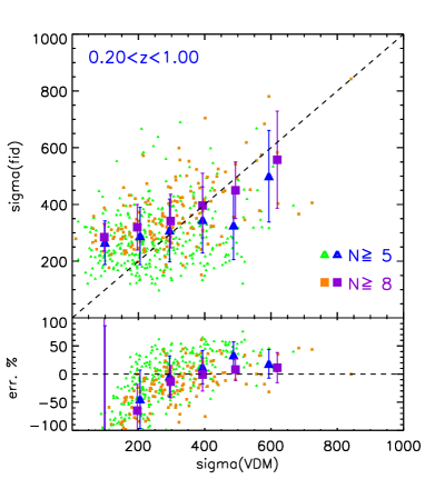
Figure 8: Comparison between virial ($y$ axis) and VDM reconstructed ($x$ axis) group velocity dispersion. Only 2 ways matches are considered in this plot. The upper panel shows the scatter plot, the lower shows the percentage error. Green and blue triangles are groups with at least 5 members, orange and purple squares groups with at least 8 members; green and orange points are single groups, while blue and purple symbols are the median (on $x$ axis) and mean (on $y$ axis) values in bins of the property on the $x$ axis. Vertical error bars are rms of mean values.

Figure 9: Mean distribution of virial line of sight velocity dispersion (continuous line), computed as the average over 20 VVDS-like mocks. The mean distribution of $\sigma$ of groups reconstructed by the VDM, averaged over the same 20 mocks, is over-plotted as black points, with vertical bars corresponding to its rms.

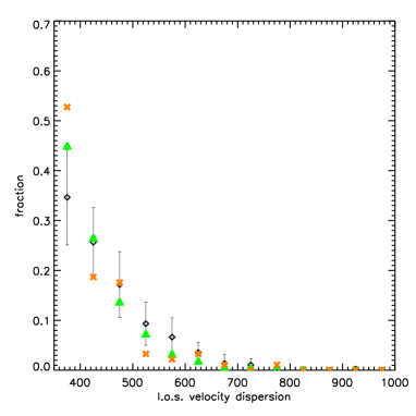
Figure 10: Normalized mean distribution of $\sigma_{VDM}$ (black diamonds) for $\sigma\geq 350$ km/s. It is the same distribution as in Figure 9, but it is normalized by the total number of groups with $\sigma\geq 350$ km/s. Overplotted green triangles represent the normalized mean $\sigma_{vir}$ distribution of fiducial groups in MILLENNIUM mock catalogue with flux limits at $I_{AB}=24$ and with 100% sampling rate ($M(100,0)$ mock catalogues, see Subsection 2.2), and the orange crosses are the normalized mean $\sigma_{vir}$ distribution of fiducial groups in complete light cones of the MILLENNIUM Simulation, i.e. catalogues with no flux limits. For each distribution, the redshift range considered is $0.2\leq z\leq 1.0$.

Sampling rate. As we applied the algorithm to the VVDS-like mocks, we optimized it for the whole observed area ($\sim 0.5$ deg² each), irrespective of the varying sampling rate across the field. Nevertheless, we tested also how completeness and purity change if computed separately in areas with very different sampling rate, that is covered by 1, 2 or 4 passes of the spectrograph (hereafter called ‘1p’, ‘2p’ and ‘4p’ areas). For this test, we assigned each group to the 1p, 2p or 4p area according to its R.A-Dec. position (computed as the median value of R.A. and Dec. of the member galaxies), even if it extends over an area with a sudden drop/increase of the sampling rate. Considering the whole redshift range $0.2\leq z\leq 1.0$, in the 4p area we find $C_{1}=0.67\pm 0.04$, $C_{2}=0.54\pm 0.04$, $P_{1}=0.55\pm 0.03$ and $P_{2}=0.48\pm 0.08$, while in the (1+2)p areas $C_{1}=0.58\pm 0.04$, $C_{2}=0.52\pm 0.04$, $P_{1}=0.57\pm 0.03$ and $P_{2}=0.49\pm 0.04$.

While $C_{2}$, $P_{1}$ and $P_{2}$ differences are inside error bars, one can notice a larger worsening in $C_{1}$ when we decrease the number of spectrograph passes, i.e. the sampling rate. Moreover, analyzing the dependence of $C$ and $P$ on group richness, we can add that in the 4p area completeness is higher even for $N\geq 5$. Moreover, we also notice that in 4p area there is a higher overmerging, especially for $N\leq 4$, while in the (1+2)p area fragmentation is increased for $N\geq 5$.

5.4 High purity parameters

With the best set of parameters, we can obtain from VVDS-02h data a group catalogue with high completeness, but it has been shown that only $\sim 50$% of groups is pure. This means that each group identified by the algorithm has, on average, only 50% probability of being a real group. It could be useful to identify the subsample of groups that has an even higher probability of being real. Thus, we optimized the group-finding algorithm a second time, in this case maximizing purity (but paying attention not to reduce the new recovered group catalogue to a few ‘super-secure’ groups). The so called high-purity parameter set is the following:

- $\mathcal{R}_{I}=0.10$ $h^{-1}$Mpc

- $\mathcal{L}_{I}=5.0$ $h^{-1}$Mpc

- $\mathcal{R}_{II}=0.6$ $h^{-1}$Mpc

- $\mathcal{L}_{II}=5.0$ $h^{-1}$Mpc

- $r=0.55$ $h^{-1}$Mpc

- $l=14.0$ $h^{-1}$Mpc

Table 2 shows $C$ and $P$ for the high-purity parameter set. Necessarily, $C$ is very low, but now each group identified by the algorithm has $\sim 70$% of probability of being real, and the interlopers fraction $f_{I}$ decreases from $\sim 40$% to $\sim 25$% with respect to the one obtained with the best set of parameters (see Table 1).

Table 2: Quality statistics ($C_{1}$, $C_{2}$, $P_{1}$, $P_{2}$, $S_{gal}$ and $f_{I}$, see text for details) of the group catalogue reconstructed by the algorithm with the high-purity parameter set, for two different redshift bins and for the whole redshift range, considering groups with N$\geq$2. Each parameter is computed as the mean over the 20 VVDS-like mocks, and the associated error is its $rms$. The same parameters for groups with N$\geq$3 are consistent, within error bars, with those presented here.

Quality statistics for N$\geq$2
Quality parameter	$0.2\leq z\leq 0.6$	$0.6\leq z\leq 1.0$	$0.2\leq z\leq 1.0$
$C_{1}$	$0.29\pm 0.03$	$0.20\pm 0.03$	$0.24\pm 0.02$
$C_{2}$	$0.24\pm 0.03$	$0.17\pm 0.02$	$0.20\pm 0.02$
$P_{1}$	$0.75\pm 0.04$	$0.73\pm 0.06$	$0.74\pm 0.04$
$P_{2}$	$0.66\pm 0.07$	$0.69\pm 0.06$	$0.67\pm 0.05$
$S_{gal}$	$0.32\pm 0.03$	$0.21\pm 0.04$	$0.28\pm 0.03$
$f_{I}$	$0.24\pm 0.04$	$0.27\pm 0.05$	$0.25\pm 0.03$

6 VVDS-02h field group catalogue

We applied the group-finding algorithm to the VVDS-02h sample described in Section 2.1, using the best set of parameters. We defined the redshift and the position in the R.A.-Dec. plane of each group as the median values of redshift, Right Ascension and Declination of the group members. Figure 11 shows the redshift distribution of the identified groups, with different line styles for different cuts in group richness, as indicated in the Figure. It is clear that beyond $z\sim 1$ there is a significant drop in the number of recovered groups, irrespectively of their richness, as expected from Figure 2. This drop in the redshift distribution may partly be related also to the choice of optimizing the algorithm only up to $z=1$ (see Section 5.2). We applied the VDM to our galaxy sample also using the high-purity set of parameters. With the best set of parameters, the algorithm identified 318 groups with 2 or more members in the redshift range $0.2\leq z\leq 1.0$, one third of them having also been detected with the high-purity set. The identified groups comprise $\sim 19$% of the galaxies in our sample. Comparing this percentage with the fraction of galaxies that reside in groups in VVDS-like mock catalogues, we found that it is consistent with both the fraction of galaxies residing in fiducial groups ($\sim 20$ %) and the percentage of galaxies residing in reconstructed groups ($\sim 22$%).

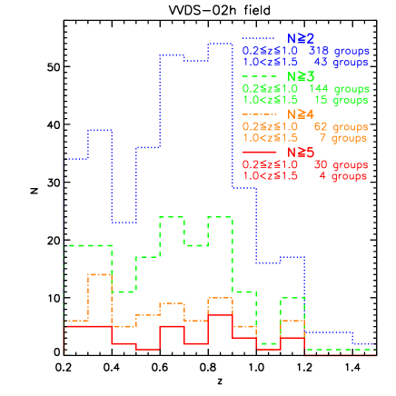
Figure 11: The redshift distribution of groups in the VVDS-02h sample, found using the best set of parameters. Different line styles are for different cuts in group richness, as indicated. The total number of groups with the corresponding richness is quoted in the labels, for two different redshift ranges.

For each group we estimated the line of sight velocity dispersion $\sigma$. We used the gapper method, as described in Section 3.2, and we corrected it for the redshift measurement error subtracting it in quadrature as in Equation 3. We set $\sigma=0$ km/s for those groups with a measured $\sigma_{G}$ (from Equation 1) lower than the redshift error. $\sim 25$% of groups with $\sigma\geq 350$ km/s have been detected by the algorithm also with the high-purity parameter set.

It is worth noticing that, given the small value of the parameter $r$, driving the projected dimension of the search cylinder in Phase III (see Section 4.3), the typical projected radius within which the full set of group members is selected is always $<1$ $h^{-1}$Mpc.

Detailed group catalogue statistics are shown in Table 3. The number of groups that has been found in VVDS-02h field is quoted. Different rows are for different values of velocity dispersion, different columns for different richnesses. Numbers in brackets indicate the number of groups that have been identified by the algorithm also with the high-purity set of parameters (even if with less members).

We tested the reliability of the reconstructed catalogue by recomputing the groups excluding galaxies with flag=2 and 9, i.e. using only galaxies whose redshift has a high likelihood ($>95$%) of being correct. We verified that, with respect to our original group catalogue, 80% (/77%/75%) of the groups with at least 5 (/4/3) members are still recovered. These means that for these recovered groups the galaxies with flag=2 and 9 were not in the seed of the group, i.e. in the first set of galaxies recovered in the Phase I of the algorithm (see Section 4.1).

Table 4 lists all the groups identified in the redshift window $0.2\leq z\leq 1.0$. It is worth noticing that the quoted number of members has to be considered as a lower limit for the real richness, as the sampling rate of our survey is not 100%. The groups labeled with a star near their ID are those recovered also when using only galaxies with flag=3 and 4. We apply this label only to groups with at least 3 members. The group members are presented in Table 5. Note that the galaxy ID is the same used to identify galaxies in the public VVDS release at http://cencosw.oamp.fr.

In Figure 12, the two-dimensional VVDS galaxy distribution is shown, with galaxy positions projected on Right Ascension and redshift. Each plot shows a different redshift bin, as quoted on the $y$ axis. Black dots are field galaxies, while coloured dots are group members (blue dots are pair members, green are triplet members, orange are quartet members and red dots are galaxies included in groups with 5 or more members).

Table 3: Number of VVDS-02h groups reconstructed by the algorithm using the best set of parameters in VVDS-02h field, for $0.2\leq z\leq 1.0$. Statistics are quoted as a function of the number of group members (columns) and of measured line of sight velocity dispersion of group galaxies ($\sigma$, in km/s, rows). Numbers in brackets indicate the number of groups found also applying the algorithm with the high-purity set of parameters.

$\sigma$ (km/s)	Group members
	2	3	4	5	6	7	8	9	ALL
$\sigma=0^{a}$	89(23)	24(10)	8(2)	-	-	-	-	-	121(35)
$0<\sigma<350$	61(25)	39(18)	18(6)	8(5)	3(2)	3(3)	2(1)	-	134(60)
$\sigma\geq 350$	24(0)	19(6)	6(3)	5(1)	4(2)	3(2)	1(0)	1(1)	63(15)
								Total:	318(110)
a) We refer the reader to Section 6 for the meaning of $\sigma=0$

Table 4: List of groups recovered in the VVDS-02h field in the range $0.2\leq z\leq 1.0$. Columns are the following: 1) group ID; 2) R.A.; 3) declination; 4) redshift; 5) number of detected members; 6) l.o.s. velocity dispersion $\sigma$; 7) possible high purity. R.A. and declination are in degrees and $\sigma$ in km/s. R.A., declination and redshift are the median values of all the galaxies in each group. The star near the group ID label those groups found by the algorithm also when using only galaxies with flag 3 and 4 (see text for further details). Column 7 labels with an ‘H’ those groups detected by the algorithm also with the high-purity set of parameters. See the electronic edition for the complete list of VVDS-02h groups.

grID	R.A.	Dec.	$z$	N	$\sigma$	Purity
	$deg.$	$deg.$			$km/s$
124∗	36.56310	-4.31748	0.5850	3	351	H
144∗	36.79910	-4.59669	0.6135	5	428	H
224∗	36.80323	-4.67940	0.7898	4	392

Table 5: List of group galaxies belonging to the groups listed in Table 4. Columns are the following: 1) galaxy ID; 2) R.A.; 3) declination; 4) redshift; 5) redshift quality flag (see Section 2.1); 6) ID of the group to which the galaxy belongs 7) total number of group members. R.A. and declination are in degrees. See the electronic edition for the complete list of VVDS-02h group galaxies.

galIDa	R.A.	Dec.	$z$	z flag	grID	N
	$deg.$	$deg.$
20309041	36.56095	-4.31812	0.5859	4	124	3
20309502	36.56310	-4.31748	0.5850	4	124	3
20310401	36.56771	-4.31544	0.5824	2	124	3
20176187	36.79656	-4.61242	0.6072	4	144	5
20183000	36.79910	-4.59744	0.6135	4	144	5
20183332	36.79801	-4.59669	0.6136	4	144	5
20184297	36.80199	-4.59303	0.6137	2	144	5
20184706	36.80420	-4.59215	0.6126	3	144	5
20146543	36.80323	-4.68008	0.7857	3	224	4
20146933	36.80903	-4.67979	0.7890	3	224	4
20147204	36.79638	-4.67940	0.7911	4	224	4
20151406	36.79351	-4.66935	0.7898	3	224	4
a) The galaxy ID refers to the public VVDS release at
http://cencosw.oamp.fr

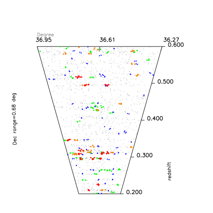
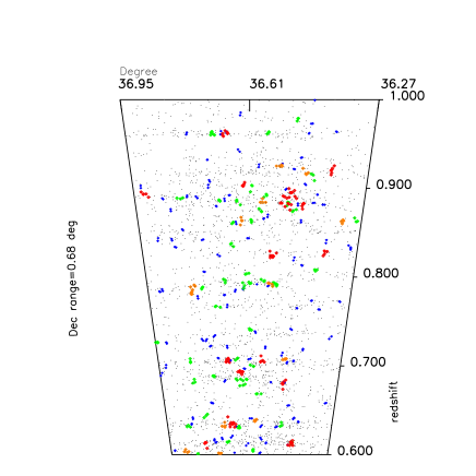
Figure 12: Two-dimensional VVDS galaxy distribution as a function of Right Ascension and redshift (points are compressed on the Declination dimension). Each plot shows a different redshift bin ($0.2\leq z\leq 0.6$ and $0.6\leq z\leq 1.0$ in upper and lower panel respectively). Black dots are field galaxies, coloured dots are group members, according to the group catalogue obtained with the best set of parameters. The colour code is the following: blue dots are pair members, green are triplet members, orange are quartet members and red dots are members of groups with 5 or more members.

6.1 Line of sight velocity dispersion of group galaxies

It is interesting to check whether the real universe looks like the simulated one. In this section we compare the VVDS catalogue with the Millennium-based mock catalogues.

We compared the $n(\sigma)$ distributions of real and simulated groups. Figure 13 shows the $n(\sigma)$ distribution for all VVDS-02h groups in the redshift range $0.2\leq z\leq 1.0$ (red triangles) and the $n(\sigma)$ distribution for VVDS-like mock catalogues. As in Figure 9, the continuous line is the distribution of $\sigma_{vir}$ of fiducial groups, while black points represent the mean distribution for reconstructed groups, with vertical bars being the rms of the 20 mock catalogues. In this plot we consider the $\sigma$ measured with the gapper method (for both mocks and real data) and not the virial velocity dispersion. Moreover, we are excluding groups with measured $\sigma$ equal to 0, because this value indicates that we have not been able to measure it due to the redshift measurement error (see Equation 3). This is the reason why the area under $n(\sigma_{vir})$ in the plot is larger than the area under the other distributions. In this Figure one can notice a consistency in the $n(\sigma)$ distributions of real and mock group catalogues, at least for $\sigma>350$ km/s.

The relatively large number of groups for which the velocity dispersion estimated through Equation 3 is formally negative is probably due to the fact that we did not take into account possible dependences of the mean redshift error on the properties of the galaxies (i.e. magnitude, presence of emission lines etc.). It is likely that for many of these groups the redshift error associated to their galaxy members is somewhat smaller than the adopted average value (275 km/s). Nevertheless, we are reassured by the fact that none of the groups with $N\geq 5$ has $\sigma=0$.

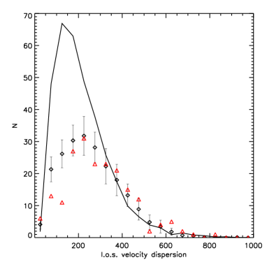
Figure 13: As in Figure 9, but in this case the velocity dispersion distribution of VVDS-02h field groups is also shown with red triangles.

6.2 Comparison with other group catalogues in the same field

Several group catalogues have already been compiled from different kind of observations and with different methods in the sky area covered by the VVDS-02h field. For example, X-ray clusters have been identified from XMM-Newton images and then spectroscopically confirmed (Andreon et al., 2004b; Valtchanov et al., 2004; Andreon et al., 2005; Willis et al., 2005a, b; Bremer et al., 2006; Pierre et al., 2006). The matched-filter technique has been used as well (Olsen et al., 2007), together with a weak lensing search (Gavazzi & Soucail, 2007) and structure identification through photometric redshift (Mazure et al., 2007). All these latter methods were applied to photometric data from CFHTLS.

Among the X-ray clusters of the XMM-LSS, only 8 clusters fall in the VVDS-02h field area in the redshift bin $0.2\leq z\leq 1.0$: XLSSC 005, XLSSC 013 and XLSSC 025 from C1 catalogue, XLSSC 038 form C2 catalogue and then the clusters a, b, c, d from C3 catalogue (see Table 3 in Pierre et al., 2006). We find that both clusters b and c have a counterpart in our VDM catalogue (with 6 and 8 detected members respectively), with an almost perfect match in their barycenters. Clusters XLSSC 013 and XLSSC 025 have possible counterparts at the same z (with 4 and 3 members respectively), but their barycenters in ra-dec have a shift of $\sim 200$ $h^{-1}$ kpc. Inspecting these two groups more in details, we find that the possible XLSSC 025 counterpart is dominated by a massive galaxy that is distant from XLSSC 025 barycenter $\sim 100$ $h^{-1}$ kpc, showing that in this case a better match would have been obtained if we had computed a mass-weighted barycenter. On the contrary, for XLSSC 013 counterpart we do not identify any dominant galaxy. This shift of $\sim 200$ $h^{-1}$ kpc could also be explained by the following: we studied the distances between the barycenters of VDM groups and their corresponding fiducial groups, and we found that their distribution is a Gaussian centered at $\sim 0$ with a scatter of $\sim 200$ $h^{-1}$ kpc. Finally, we do not find counterparts for XLSSC 005, XLSSC 038, a and d in our catalogue. They fall inside our low sampling rate areas (covered only by 1 or 2 passes of the spectrograph), and a further inspection confirmed that the sampling rate in those regions does not allow our algorithm to find at least two galaxies inside the volume enclosed in the Phase I cylinder.

We concluded this comparison with XMM-LSS detections inspecting the relation between optical and X-ray properties of the four groups for which there exists a (possible) XMM counterpart. In particular, we considered the relation between the X-ray luminosity $L_{X}$ presented in Table 5 of Pierre et al. (2006) and the velocity dispersions $\sigma$ we have measured. We verified that groups XLSSC 013, $b$ and $c$ have a $\sigma$-$L_{X}$ relation well in agreement with the linear fit in the plane $\sigma$-$L_{X}$ presented in Figure 13 of Popesso et al. (2005). For group XLSSC 025 we measure a $\sigma$ that would be too low for its quoted $L_{X}$, according to the shown relation, but as its $\sigma$ is of the order of 200 km/s it does not reside in the $\sigma$ range that we consider reliably measured.

It is worth noticing that our richest groups (10 groups with at least 7 members) do not match with XMM-LSS clusters, except one that is the counterpart of the X-ray selected group c. There are at least three reasons why an optical group may have not been detected in X-ray: a) it may falls on the boundaries of a XMM-LSS pointing, thus in a region where the X-ray detector is affected by vignetting; b) it may have a redshift much higher than the mean $z$ reachable by the performed X-ray observations; c) it may have a low surface brightness, that corresponds to a shallow potential well of the mass distribution, thus making X-ray detection more difficult. We inspected our richest groups, and we found that all of them fall in at least one of these three categories. In particular, we verified that the $N(z)$ distribution of all X-ray clusters in the above-cited works is peaked at $z\sim 0.4$, while the $N(z)$ distribution of our richest groups is quite flat and reaches $z\sim 0.9$, with 5 groups with $z\geq 0.7$. Moreover, at least half of our richest groups do not have a dominant member, that is a galaxy with luminosity and/or stellar mass much higher than the others. The VVDS-02h field sampling rate could be enough to explain this lacking of dominant galaxies, but in principle we can not reject the hypothesis that the dominant galaxy in (some of) these groups may not exist, and in this latter case we are allowed to think that these groups have a real low X-ray surface brightness.

We compared our group catalogue also with the ones in Gavazzi & Soucail (2007), Olsen et al. (2007) and Mazure et al. (2007).

Among the about 20 clusters in Olsen et al. (2007) that are inside the sky area and redshift range that we have explored, roughly half fall inside regions with too low sampling rate for our Phase I cylinder to be able to detect at least a pair; two of them (ID 30 and 42) fall very near in redshift to two wide structure at $z\sim 0.32$ and $z\sim 0.45$ , within which our algorithm detects (possibly fragmenting them) a few groups. Finally, considering the depth of the redshift bins in which Olsen’s groups can reside ($\Delta z\sim 0.1$) due to the use of photometric redshifts, we find that for 5 groups in Olsen’s catalogue there exists a counterpart in our catalogue.

Among the about 30 structures detected by Mazure et al. (2007) in the redshift range $0.2<z<1.0$, we find that about 20 fall inside regions with too low sampling rate for our finding group algorithm (13 of which in the 1 pass area); a few of them reside in redshift slices ($z\sim 0.3$, $z\sim 0.7$ and $z\sim 0.9$) where a wide (in ra-dec) structure is also present, that has been possibly fragmented by our algorithm, producing in our catalogue more than one counterpart. Finally, three of the structures detected by Mazure et al. (2007) have a possible direct counterpart in our catalogue (general ID 5, 19 and 21, see Table 3 in Mazure et al., 2007).

Finally, the 3 structures detected by Gavazzi & Soucail (2007) and that fall inside VVDS-02h field are in very low sampling rate areas, thus in regions where our algorithm did not detect any group.

In this comparison we also took into account that in the CFHTLS data that have been used in the three above-mentioned works there are masked sky regions that have not been used for group finding, as it is shown for example in Figure 1 in Mazure et al. (2007) and Figure 9 in Olsen et al. (2007). We find that $\sim 5$% of our groups in the range $0.2\leq z\leq 1.0$ fall in those regions. Moreover, we observe that roughly half of this masked area falls inside the region that in VVDS-02h field has the highest sampling rate (the central area highlighted in Figure 1), and that this higher-sampling region covers only $\sim 25$% of the VVDS-02h field. Thus, the percentage of our groups falling in the masked areas increases to $\sim 8$% for groups with at least 3 members and to 20% for our 10 richest groups (those with at least 7 members).

7 The U-B colour of group galaxies

Having reconstructed a catalogue of groups at high $z$, we want now to use it to study the dependence of galaxy properties on environment, and also its evolution with cosmic time. More specifically, we aim at investigating if physical properties of group galaxies are different from the properties of the entire sample of galaxies, up to $z\sim 1$. Are the relations that we see in groups at low redshift already present at $z\sim 1$? Is there any unambiguous signature of time evolution in known scaling relations characterizing galaxies in cluster environments? In this paper, we will not carry on an exhaustive analysis of this topic, that will be possibly the goal of a future work. The main aim of this paper is to present the VVDS-02h field group catalogue and discuss its reliability. So, in this Section we simply want to show the potentiality of our group catalogue for studies related to environmental effects on galaxy properties on group scales.

As we want to investigate the redshift evolution of the properties of group galaxies, we have to study a group sample homogeneous at all $z$. We thus require that the groups we use for this analysis have at least two members brighter than a luminosity limit that allows us to be complete up to $z=1$. This luminosity limit evolves with redshift. Following roughly the evolution of $M^{*}$, the characteristic magnitude of the luminosity function (Ilbert et al., 2005), we set this limit as $M_{B}\leq-18.9-1.1z$. Our ‘group galaxy’ sample is composed by those galaxies, brighter than this limit, in groups with at least two members brighter than this limit itself. Moreover, we define a ‘total’ galaxy sample considering all galaxies brighter than this limit (including also those in groups).

Once defined the sample, as a first step we studied the fraction of ‘blue’ galaxies ($f_{b}$ from now on) in both the group and total samples, in the range $0.2\leq z\leq 1.0$. The general blueing of cluster galaxy population for increasing redshift, first shown by Butcher & Oemler (1978) and Butcher & Oemler (1984) and known as the Butcher-Oemler effect, has been widely confirmed in following studies (see for example Margoniner et al., 2001; De Propris et al., 2003; Gerke et al., 2007). Nevertheless, nowadays there is no full agreement about the origin of this blueing. It can be related to environmental effects (e.g. Dressler et al., 1997), but it has also been suggested that it is consistent with the overall ageing of all galaxies, irrespective of their environment (Andreon et al., 2004a, 2006).

According to our criteria, a galaxy is ‘blue’ if it has a colour $U-B\leq 1$. This threshold has been chosen as it corresponds roughly to the minimum (i.e. the green valley) in the bimodal $U-B$ colour distribution. Moreover, this colour cut has been kept constant at all redshifts as we found that the green valley colour does not evolve much in the $z$ range considered. For the computation of the $U$- and $B$-band absolute magnitudes we refer the reader to Ilbert et al. (2005).

Since our goal is to study $f_{b}$ as a function of redshift, we first verified that the failure rate in redshift measurement does not depend on redshift for specific galaxy colours. We assigned to each galaxy a “photometric type” according to the scheme proposed by Zucca et al. (2006). The classification is carried out by fitting the Spectral Energy Distribution of galaxies to six templates (four observed spectra, Coleman et al., 1980, and two starburts SEDs, Bruzual A. & Charlot, 1993). We then proceeded as in Franzetti et al. (2007), by defining a broad bimodal classification. We considered E/S0 and early spirals as ‘early type’, and late-type spirals, irregular and starburst types as a ‘late-type’. The relation between this classification scheme and the colour U-B that we use to compute $f_{b}$ is monotonic, with bluer colours being associated to ‘late type’ templates. In particular, our ‘early type’ population constitutes $>90$% of the galaxies with $U-B>1$. We computed the ‘late type’ galaxy fraction in both our spectroscopic sample and in the photometric parent catalogue, in three redshift bins in the range $0.1\leq z\leq 1.0$ (using photometric redshifts for the parent catalogue, see Section 2.1 for their determination). As already found by Franzetti et al. (2007), who carried on a similar analysis on wider redshift intervals up to $z\sim 2$, the ‘late type’ fraction is $\leavevmode\nobreak\ 3$% higher in the spectroscopic sample and this increment does not depend on redshift. This result implies that any trend of $f_{b}$ with redshift is not due to a measurement bias in our sample.

Figure 14 shows $f_{b}$ for the group galaxies (blue triangles) in three different redshift bins: $0.2\leq z\leq 0.5$, $0.5\leq z\leq 0.7$ and $0.7\leq z\leq 1.0$. The vertical error bars are the $1\sigma$ confidence levels associated to $f_{b}$, computed with the usual approximation of the formula for binomial statistics given in Gehrels (1986): $\sigma^{2}=f_{b}f_{r}/n$, where $f_{r}=1-f_{b}$ and $n$ is the total number of galaxies in the redshift bin.

As reference, we plot the linear fit of the three points as a blue line, while the upper black line is the linear fit for $f_{b}$ computed within the ‘total’ sample. $f_{b}$ is clearly lower in groups than in the total sample. The slopes of the two fits, together with their $1\sigma$ confidence levels, are $0.27\pm 0.07$ and $0.15\pm 0.02$ for the group and total sample respectively. Although they are both significantly different from zero, and the group slope is steeper, they are compatible with each other, the group sample slope being steeper only at a $1.6\sigma$ significance level. At this stage of investigation we are only able to confirm the different overall value of $f_{b}$ between group galaxies and the total sample, but not their possible different evolution. We verified that these results are stable against the variation of the U-B threshold adopted to define blue galaxies (by $\pm 0.05$ mag). They did not change significantly also when we implemented a colour cut that depends on luminosity, following the mild dependence on magnitudes of the green valley locus. Although we do not detect any redshift dependence of the green valley locus up to $z=1$, we also allowed the colour cut to vary by 0.1 mag redward for any redshift decrease of $dz=1.0$ (as suggested by Blanton, 2006 and as adopted by Gerke et al., 2007). As a matter of fact, even in this case the two slopes are appreciably different from zero, and their relative difference significant at the $\sim 1.5\sigma$ level.

We compared our results with those presented by Gerke et al. (2007), who studied the fraction of blue galaxies in groups and in the field within different subsamples extracted from the DEEP2 data set. In their Sample I, the one with a selection most similar to ours, they find that $f_{b}$ is lower in groups than in the field, but they do not detect any significant evolution of $f_{b}$ with $z$ neither in groups nor in the field. Anyway, evolutionary effect are much more difficult to quantify in that sample since the redshift range as well as the luminosity range covered is narrower with respect to that explored in this study.

Our results are in agreement with those presented by Iovino et al. (2010), who studied the evolution of $f_{b}$ in groups and in the field within the zCOSMOS-10k sample (see also, for completeness, the analysis of Kovac et al., 2009 concerning the fraction of early type galaxies in groups). This agreement is based on the comparison with their Sample II, the one with a luminosity cut most similar to ours, and it holds for both the group and the total sample. Interestingly, Iovino et al. (2010) find that in their luminosity limited sample galaxy colour still depends on environment at $z\sim 1$ (with a trend similar to what we find in this work), but at the same redshift they do not converge to the same conclusion when the blue fraction is recovered from a (stellar) mass limited sample ($\log(M/M{\odot})\geq 10.8$). They explain this result suggesting that red galaxies of such stellar masses, already in place at $z\sim 1$, may rise from internal mechanisms of evolution, on which environment has no influence. We refer the reader to Iovino et al. (2010) for more details.

Cucciati et al. (2006) carried on a similar analysis using the same VVDS-02h data set that we use in this work. They studied the colour-density relation up to $z=1.5$, with the local density computed within Gaussian filters with $\sigma=5$ h^-1Mpc. They found that the colour-density relation becomes weaker for increasing redshift (the evolution of $f_{b}$ being faster in high densities), and that at $z\sim 1$ no significant colour-density relation is detected, for galaxies with $M_{B}\leq-20$ (that is equivalent to the threshold we use in this work). Taken at face value, our results are not compatible with these previous findings, as we find that at $z\sim 1$ $f_{b}$ is still different in groups and in the total sample. This difference can be explained with the fact that we are exploring higher densities/smaller scales ($<1$ $h^{-1}$Mpc, see Section 6). For example, there are several studies in literature suggesting that environmental effects on large scales are only a weaker residual of the ones acting on smaller scales (e.g. Kauffmann et al., 2004; Blanton et al., 2006). The same hypothesis is suggested by Cooper et al. (2007), when comparing the colour-density relation found in the DEEP2 data set with the one presented in Cucciati et al. (2006). They still find a colour-density relation at $z\sim 1$, but on smaller scales than those investigated by Cucciati et al. (2006).

A direct comparison of results obtained on the basis of heterogeneous definitions of the local environment (as for example density field maxima as opposed to groups) is not straightforward. Cooper et al. (2007) showed, for example, that the evolution of the colour-density relation is continuous in the range $0.4<z<1.3$, while Gerke et al. (2007), who used the same DEEP2 data set but a different definition of environment based on groups, found that the evolution of $f_{b}$ in groups is flat in the range $0.7<z<1.0$, and it steepens for $1.0<z<1.3$. Nevertheless, the two works agree on the fact that at $z\sim 1.3$ the colour-density relation seems to disappear. No need to emphasize that the physics associated with different environmental definition has still to be fully understood.

Also a direct comparison of our results with those presented in other works up to $z\sim 1$ is not trivial. Interpretation is hampered by the the non-homogeneity of group catalogues selected according to different selection criteria. As a consequence, the picture emerging from these studies is complex and sometimes even contradictory. As this Section is meant to give a general idea of the kind of studies that can be potentially carried out with our group sample, we will not enter in details. We rather refer the reader to Poggianti et al. (2006) and Andreon et al. (2006) for a more in-depth discussion about the status of the art and the problems related to uncontrolled selection effects.

As a second step, we examined the behavior of $f_{b}$ in groups characterized by different degrees of richness. There is still no agreement in literature about the dependence of $f_{b}$ on cluster properties. For example, $f_{b}$ is found both to depend on cluster richness (Margoniner et al., 2001; Goto et al., 2003), or to be independent of it, as well as of line of sight velocity dispersion and mass (De Propris et al., 2004; Goto, 2005; Popesso et al., 2007b). To address this issue, we associated to each group the number of members found by the algorithm. Nevertheless, due to the survey characteristic (sampling rate, spectra signal to noise ratio, etc.), the observed number has to be corrected to recover the real number of members within the flux limit of the survey ($I_{AB}\leq 24$). We did this by weighting each galaxies with the ‘target sampling rate’ and the ‘spectroscopic success rate’ of the survey (see Ilbert et al., 2005). We then modulated this mean weight with a finer correction which takes into account that the sampling rate is not uniform in the field. This is done by using the $\Psi(\alpha,\delta)$ selection function described in Cucciati et al. (2006). This way, for each group we computed a corrected richness ($N_{c}$), which is the sum of the weights of those galaxies brighter than the evolving luminosity limit described above. In Figure 14, green diamonds, orange squares and red stars show $f_{b}$ within groups with $N_{c}\geq$ 7, 14 and 20. We can see in the plot a general trend of decreasing $f_{b}$ for increasing $N_{c}$, at any redshift explored. Given the error bars, this decrement is not significant when considering single steps in $N_{c}$, but the overall tendency is clear. Nevertheless, it does not seem that the $f_{b}$ redshift evolution is different for different values of $N_{c}$. These results are in agreement with those found by Iovino et al. (2010) in their analysis of the zCOSMOS-10k group sample, but we extended them to fainter magnitudes. It would be indeed interesting to study the dependence on $N_{c}$ also for other galaxy properties, as it has been done for example for star formation rate (SFR) and specific SFR (see for example Popesso et al., 2007b). This could give hints on how different galaxies properties may be affected by different environments. We defer this study to a future work.

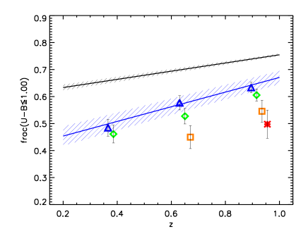
Figure 14: Fraction of blue galaxies ($U-B\leq 1$) for group galaxies (blue empty triangles) in three different redshift bins: $0.2\leq z\leq 0.5$, $0.5\leq z\leq 0.7$ and $0.7\leq z\leq 1.0$. The linear fit of this three points is overplotted as a blue line, while the upper black line is the linear fit for $f_{b}$ computed within the ‘total’ sample. he dashed areas along the two linear fits show the locus where the linear fits could lie considering their 1-$\sigma$ error on both intercept and slope. See text for more details. Other symbols are for group galaxies in groups with increasing corrected richness: $Ncorr\geq 7,14,20$ for green diamonds, orange squares and red stars respectively.

8 Summary and conclusions

We have compiled a homogeneous catalogue of optical groups identified in the VVDS-02 field by means of the VDM algorithm, in the range $0.2\leq z\leq 1.0$.

We used mock catalogues simulating the VVDS survey to optimize the performances of the group-finding algorithm (maximizing the completeness and the purity of the resulting group catalogue) as well as to minimize possible selection effects. Our main results are here summarized.

• Using the mock catalogues, we verified that the VVDS-02h survey sampling rate allows us to recover at least $50$% of the groups (with a virial line of sight velocity dispersion $\sigma_{vir}\geq 350$ km/s) that are potentially present in the parent photometric catalogue up to $z=1$.

• We tested how well $\sigma_{vir}$ of the halo mass particles can be estimated using sparsely sampled galaxy velocities. We verified that with this method, given the characteristics of our survey (flux limit, sampling rate, redshift measurement error) we are able to recover a sensible value of $\sigma_{vir}$ for $\sigma_{vir}\geq 350$ km/s.

• Applying the optimized algorithm to the VVDS real data set, we obtained a catalogue of 318 groups of galaxies (with at least two members) in the range $0.2\leq z\leq 1.0$. Among these groups, 63 have a measured line of sight velocity dispersion greater than 350 km/s. The group catalogue is characterized by an overall completeness of $\sim 60$% and a purity of $\sim 50$%. Nearly $19$% of the total population of galaxies live in these systems.

• the number density distribution as a function of both redshift ($n(z)$) and velocity dispersion ($n(\sigma)$) of the VVDS groups with $\sigma>350$ km/s scales in qualitative agreement with the analogous statistics recovered from the mock catalogues.

• We studied the fraction $f_{b}$ of blue galaxies ($U-B\leq 1$) in the range $0.2\leq z\leq 1$. We used a luminosity-limited subsample of galaxies extracted from our data ($M_{B}\leq-18.9-1.1z$), complete up to $z=1$. We found that $f_{b}$ is significantly lower in groups than in the global galaxy population. Moreover, $f_{b}$ increases as a function of redshift irrespectively of the environment, with marginal evidence for a faster growth rate in groups. We also analysed how $f_{b}$ varies as a function of group richness, finding that, at any redshift explored, $f_{b}$ decreases in systems with increasing richness.

Further explorations of the properties of VVDS groups is left to future works. We only anticipate that the high degree of completeness of the catalogue can be potentially exploited for extracting cosmological information via, for example, cluster counts techniques. The high level of purity makes the VVDS group sample ideal also for astrophysical studies which aim at tracing various physical properties of galaxies as a function of local density and environment. We also mention that the cross-correlation studies of our optically-selected catalogue with samples inferred in the same field with independent techniques will help to gain insights not only on cluster selection biases but also on the physics at work within these extreme environments.