Magnetic impurity resonance states and symmetry of the superconducting order parameter in iron-based superconductors

Abstract

We investigate the effect of magnetic impurities on the local quasiparticle density of states (LDOS) in iron-based superconductors. Employing the two-orbital model where 3$d$ electron and hole conduction bands are hybridizing with the localized $f$-orbital of the impurity spin, we investigate how various symmetries of the superconducting gap and its nodal structure influence the quasiparticle excitations and impurity bound states. We show that the bound states behave qualitatively different for each symmetry. Most importantly we find that the impurity-induced bound states can be used to identify the nodal structure of the extended $s$-wave symmetry ($S^{\pm}$) that is actively discussed in ferropnictides.

I Introduction

The problem of magnetic impurities in a superconductor has been extensively discussed in the literatureShiba68 ; Matsumoto02 ; Sakai93 ; Satori92 ; Balatsky06 . The magnetic impurity and its moment can interact with the conduction electrons of the metal in the normal or superconducting state. In the former case this leads to the Kondo effect and a resonance state at the Fermi level. In the latter case it is well known that a single magnetic impurity doped into a superconductor produces a localized bound state within the quasiparticle excitation gapShiba68 . The spectrum is sensitive to the symmetry of the order parameter and is therefore a powerful tool to probe the pairing symmetry.

The discovery of new Fe-based superconductorsKamihara08 with distinct multi-orbital band structure Bruning08 ; Zhao08 ; Pourovskii08 have opened a new horizon to high temperature superconductivity. One of the most significant questions for these materials is the symmetry of the superconducting gap and the underlying Cooper-pairing mechanism. The latter is believed to arise due to purely electronic mechanism and a variety of models have been investigated with various weak-coupling approaches within random phase approximation RPA Kuroki08 ; Maier09 ; Schmalian09 and renormalization group techniques Chubukov08 ; Zhai09 . It was concluded that the fully gapped extended s-wave state with the $\pi$-shift of the gap between electron and hole Fermi surface sheets is the most natural outcome of these theories. It is believed to be driven by the interband spin fluctuations at the antiferromagnetic wave vector $(\pi,\pi)$ in folded Brillouin zone and it also competes with the spin density wave instability at the same wave vector which leads to the columnar or striped AF state for low doping.

However, despite intensive experimental efforts, the pairing symmetry of this new class of superconducting materials is not completely settled. Some experimental groups have reported the fully gapped behavior Lue09 ; Hashimoto09 ; Malone09 ; Khasanov08 ; Zhang01 , but some measurements, in particular NMR relaxation and penetration depth suggest existence of gap nodes Nakai08 ; Shan08 ; Mu08 . From the theoretical side it has also been realizedvavilov ; Maier09 that the superconducting gap structure may be non-universal in ferropnictides due to the large intraband Coulomb repulsion. Its inclusion may force the superconducting gap to develop a node which crosses one of the Fermi surfaces. At the same time the symmetry of the superconducting gap will, however, still remain extended $s$-wave though higher harmonics are acquired. Moreover, in some scenariosmoreo ; kuroki the superconducting gap even changes from the extended $s$-wave towards either $d_{x^{2}-y^{2}}$- or $d_{xy}$-wave symmetries depending on the slight variation of parameters. Recently it has been found that isoelectronic substitution of As by P in BaFe₂(As_1-xP_x)₂ changes the gap structure in Fe pnictide compounds from nodeless to nodal Hashimoto09 . It seems that whereas electron- and hole doping leads to a fully gapped state, isoelectronic doping (equivalent to chemical pressure) leads to the presence of line nodes in the gap function. Therefore it is desirable to investigate the magnetic impurity effect in Fe pnictide compounds for different candidates of gap symmetries. The resulting characteristics of the LDOS which is sensitive to the nodal structure may provide a clue to distinguish between the various proposed gap symmetries. In previous investigations for FeAs compounds the effect of nonmagnetic impurities on the quasiparticle spectrum in the $S^{\pm}$ state Matsumoto09 ; Zhang09 has been studied. Magnetic impurity effects have so far only been discussed for the single band model with d${}_{x^{2}-y^{2}}$ order parameter Zhang01 , and for the two-band model for a classical local momentTsai09 . At the same time, it is known that the local density of state around the magnetic impurity can provide significant information on the local electronic structure in the unconventional superconductorhudson . Note also that the influence of nonmagnetic Senga08 ; Onari09 and magnetic Li09 impurities on the reduction of superconducting transition temperature has been recently analyzed.

In this paper we investigate the effect of a single magnetic impurity on the local quasiparticle excitations around the impurity site. We use a minimal two-band model for the electronic structure of Fe pnictides which leads to the $\Gamma(0,0)$- centered hole and M $(\pi,\pi)$-centered electron pockets. In section II the Anderson model with a strong Hubbard repulsion for the localized f-electron at the impurity site, and a hybridization between conduction bands and localized state will be introduced. We will treat this model in the infinite U limit where a slave boson representation may be used similar to Ref. Zhang01, where the Anderson impurity in the single band model with d${}_{x^{2}-y^{2}}$ order parameter has been studied. We then calculate the local density of states (LDOS) and discuss the signatures of possible Fe pnictide order parameter symmetry in its spectral and spatial characteristics. This quantity is accessible in STM tunneling spectroscopy Balatsky06 . The numerical results for the various cases will be discussed in section III. Finally in section IV we give a summary of our results and a conclusion.

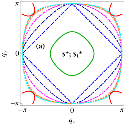
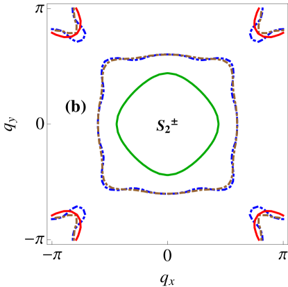
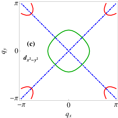
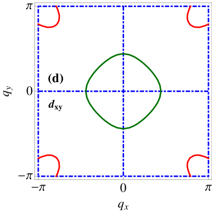
Figure 1: (color online) Fermi surfaces of the two-band model (red and green thick curves) with different symmetry of the superconducting order parameters (nodal lines represented by the dashed lines). (a) extended s-wave symmetry, starting from fully gapped $\Delta_{S^{\pm}}(k_{x},k_{y})$ (or $\Delta_{S_{1}^{\pm}}(k_{x},k_{y})$ with $\alpha=0$). With increase of the higher harmonics, $\alpha=1,3,6,7,8$ in $\Delta_{S_{1}^{\pm}}(k_{x},k_{y})$ this gap becomes more anisotropic and finally has accidental nodes on the electronic pocket around the M-point; (b) refers to the other extended nodal s-wave gap symmetry $\Delta_{S_{2}^{\pm}}(k_{x},k_{y})$ with two separate nodal lines: $\Delta_{S_{2}^{\pm}}(k_{x},k_{y})$ for $\alpha=1.2;\;\alpha^{\prime}=0.15$ and $\alpha=1.17;\;\alpha^{\prime}=0.08$); (c)-(d) show $d_{x^{2}-y^{2}}$ and $d_{xy}$ gap symmetries with symmetry enforced nodes.

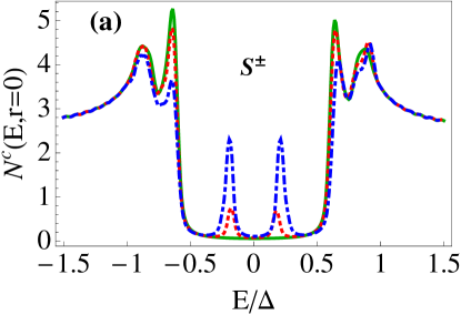
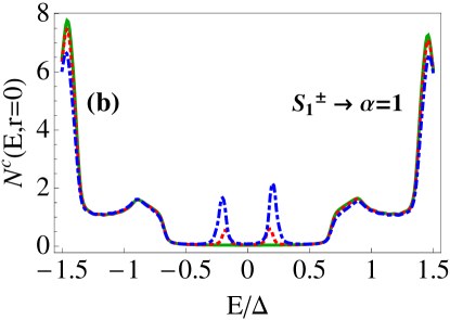
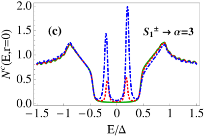
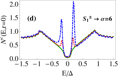
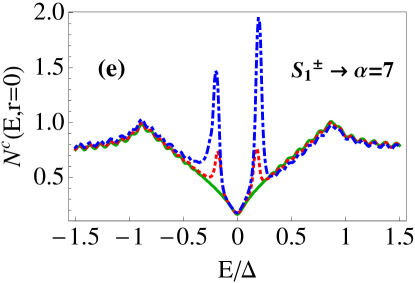
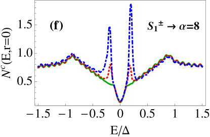
Figure 2: (color online) Calculated local density of states (LDOS) for the superconducting regime with various superconducting order parameters: a) $S^{\pm}$: $\Delta_{S^{\pm}}(k_{x},k_{y})$ and (b)-(f) $S_{1}^{\pm}$: $\Delta_{S_{1}^{\pm}}(k_{x},k_{y})$ (with $\alpha=1,3,6,7,8$ respectively); for $\epsilon_{f}=-\Delta_{0}/3$, $V_{1}=V_{2}=0$ (green), $V_{1}=V_{2}=0.5\Delta_{0}$ (red), and $V_{1}=V_{2}=\Delta_{0}$ (blue).

II Theoretical Model

According to the band structure calculationsLDA as well as numerous ARPES resultsarpes the Fermi surface topology of iron-based superconductors consists of the small size circular hole and elliptic electron Fermi surface pockets centered around the $\Gamma-$ and $(\pi,\pi)$-points of the folded BZ, respectively. The pockets are nearly of the same size which results in the nesting properties of the electron and hole bands at the antiferromagnetic wave vector, ${\bf Q}_{AF}$, ı.e. $\varepsilon_{\bf k}^{e}=-\varepsilon_{\bf k+Q_{AF}}^{h}$. Despite the fact that there are two electron and two hole pockets it has been arguedChubukov08 that it is enough to consider only two of them (one electron and one hole pocket) because the instabilities of the two-band model are the same as in the four-band model. Following this suggestion we consider two bands that are given by diagonalized tight binding expression including hoppings up to the next nearest neighbors:

$${\cal H} = \sum\limits_{{\bf k}\gamma\sigma}\varepsilon_{{\bf k}\gamma}c_{{\bf k}\gamma\sigma}^{\dagger}c_{{\bf k}\gamma\sigma}+\sum\limits_{{\bf k}\gamma}\Delta_{{\bf k}}\left(c_{{\bf k}\gamma\uparrow}^{\dagger}c_{-{\bf k}\gamma\downarrow}^{\dagger}+h.c.\right)$$ (1)

$$+\epsilon_{f}\sum\limits_{\sigma}f_{\sigma}^{\dagger}f_{\sigma}+\sum\limits_{{\bf k}\gamma\sigma}V_{{\bf k}\gamma}\left(c_{{\bf k}\gamma\sigma}^{\dagger}f_{\sigma}+h.c.\right)$$

$$+Uf_{\uparrow}^{\dagger}f_{\uparrow}f_{\downarrow}^{\dagger}f_{\downarrow}\quad,$$

where $c_{{\bf k}\gamma\sigma}^{\dagger}$ creates an electron with spin $\sigma$ in band $\gamma$ ($\gamma=1,2$ refer to the electron and hole band, respectively) with wave vector ${\bf k}=(k_{x},k_{y})$. The dispersion $\varepsilon_{{\bf k}\gamma}$ is then given in the tight-binding formKorshunov08

$$\varepsilon_{{\bf k}1} = -0.18+0.16\left(\cos k_{x}+\cos k_{y}\right)-0.052\cos k_{x}\cos k_{y}$$

$$\varepsilon_{{\bf k}2} = 0.68+0.38\left(\cos k_{x}+\cos k_{y}\right)-0.8\cos\frac{k_{x}}{2}\cos\frac{k_{y}}{2}.$$

Here, $\varepsilon_{{\bf k}1}$ dispersion yields the hole Fermi surface pocket around the $\Gamma$ point and $\varepsilon_{{\bf k}2}$ gives the elliptic electron Fermi surface pocket around the $M=(\pi,\pi)$ point, see Fig.1. The parameters have been chosen from the available fit to the ARPES data Nakayama09 (all in eV) and correspond to the hole doping of about 10$\%$. The $f_{\sigma}^{\dagger}$ operator create the localized electron at the impurity site at the origin and $U$ is its on-site Coulomb repulsion. Finally $\epsilon_{f}$ is the f-band position, $V_{{\bf k}\gamma}$ is the hybridization energy between localized electron and the conduction bands, and $\Delta_{{\bf k}}$ is the singlet superconducting gap function. We choose values for $\epsilon_{f}$, and $V_{{\bf k}\gamma}$ (Fig.2) such that the f-orbital is almost filled ($n_{f}=1$).

Our model assumes the limit $U\rightarrow\infty$ where doubly occupied f-states are excluded. This limit may be represented by introducing the auxiliary boson $b$, with the constraint $\tilde{Q}=b^{\dagger}b+\sum_{\sigma}f^{\dagger}_{\sigma}f_{\sigma}=1$Col84 . In the mean field approximation ($b=\langle b\rangle=\langle b^{\dagger}\rangle$), the total Hamiltonian including the constraint is given by ${\cal H}_{MF}+\lambda(b^{2}-1)$. Here ${\cal H}_{MF}$ is obtained as

$${\cal H}_{MF}=\widehat{\varphi}^{\dagger}\beta_{0}\widehat{\varphi}+\sum\limits_{{\bf k}}\hat{\psi}_{{\bf k}}^{\dagger}\beta_{1}({\bf k})\hat{\psi}_{{\bf k}}+(\hat{\psi}_{{\bf k}}^{\dagger}\beta_{2}\widehat{\varphi}+h.c.),$$ (3)

where $\lambda$ is the Lagrange multiplier for enforcing the constraint. The Nambu spinors are denoted by

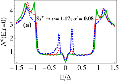
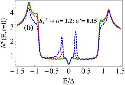
Figure 3: (color online) LDOS for the superconducting state with various order parameters: $\Delta_{S_{2}^{\pm}}(k_{x},k_{y})$ for ($\alpha=1.2;\;\alpha^{\prime}=0.15$) and ($\alpha=1.17;\;\alpha^{\prime}=0.08$); for $\epsilon_{f}=-\Delta_{0}/3$, $V_{1}=V_{2}=0$ (green), $V_{1}=V_{2}=0.5\Delta_{0}$ (red), and $V_{1}=V_{2}=\Delta_{0}$ (blue).

$\hat{\psi}_{{\bf k}}^{\dagger}=(c_{{\bf k}1\uparrow}^{\dagger},c_{-{\bf k}1\downarrow},c_{{\bf k}2\uparrow}^{\dagger},c_{-{\bf k}2\downarrow})$, and likewise $\qquad\widehat{\varphi}^{\dagger}=(f_{\uparrow}^{\dagger},f_{\downarrow},f_{\uparrow}^{\dagger},f_{\downarrow})$, while the matrices $\beta_{i}$ are defined as

$$\beta_{0}={\tilde{\epsilon}_{f}}\varsigma_{0}\otimes\sigma_{z};$$

$$\beta_{1}({\bf k})=\left[\frac{1+\varsigma_{3}}{2}\otimes\left(\varepsilon_{{\bf k}1}\sigma_{z}+\Delta_{{\bf k}}\sigma_{x}\right)\right.+$$

$$\hskip 56.9055pt\left.\frac{1-\varsigma_{3}}{2}\otimes\left(\varepsilon_{{\bf k}2}\sigma_{z}+\Delta_{{\bf k}}\sigma_{x}\right)\right];$$

$$\hskip 14.22636pt\beta_{2}({\bf k})=\left[{\tilde{V}_{{\bf k}1}}\frac{1+\varsigma_{3}}{2}+{\tilde{V}_{{\bf k}2}}\frac{1-\varsigma_{3}}{2}\right]\otimes\sigma_{z}.$$ (4)

Here $\sigma_{i}$ are the Pauli matrices acting in spin space, $\varsigma_{i}$ are the Pauli matrices in the orbital space, and $\varsigma_{i}\otimes\sigma_{j}$ denotes a direct product of the matrices operating on the 4-dimensional Nambu space. Furthermore ${\tilde{\epsilon}_{f}}=(\epsilon_{f}+\lambda)/2$, and $\bar{V}_{{\bf k}\gamma}=bV_{{\bf k}\gamma}$ are effective hybridization and energy position of the impurity $f$-level, respectively.

The local density of states (LDOS) near the magnetic impurity is obtained from analytic continuation $i\omega_{n}\rightarrow E+i0^{+}$ according to

$$N^{c}(E,{\bf r}) = -\frac{1}{\pi}Im\left[G^{c}_{11}({\bf r},{\bf r},\omega_{n})+G^{c}_{33}({\bf r},{\bf r},\omega_{n})\right],$$ (5)

where $\omega_{n}=\pi T(2n+1)$ is the Matsubara frequency, and $G^{c}(r,r^{\prime},\omega_{n})$ is a Fourier transformation of the matrix of the conduction electrons Green’s function.

The matrix Green’s functions are defined as the imaginary-time ordered average

$$G^{c}({\bf k},{\bf k}^{\prime};\tau) = -\langle T_{\tau}\hat{\psi}_{{\bf k}}(\tau)\hat{\psi}_{{\bf k\prime}}^{\dagger}(0)\rangle;$$

$$G^{fc}({\bf k};\tau) = -\langle T_{\tau}\widehat{\varphi}(\tau)\hat{\psi}_{{\bf k}}^{\dagger}(0)\rangle;$$

$$G^{cf}({\bf k},\tau) = -\langle T_{\tau}\hat{\psi}_{{\bf k}}(\tau)\widehat{\varphi}^{\dagger}(0)\rangle;$$

$$G^{f}(\tau) = -\langle T_{\tau}\widehat{\varphi}(\tau)\widehat{\varphi}^{\dagger}(0)\rangle.$$ (6)

Where $G(\tau)=T\sum_{\omega_{n}}G(\omega_{n})e^{-i\omega_{n}\tau}$. At low temperature regime $T\sum_{\omega_{n}}(\ldots)\longrightarrow\frac{-1}{\pi}Im\int_{0}^{D_{\gamma}}d\omega\lim\limits_{i\omega\rightarrow\omega+i0^{+}}(\ldots)$, where $D_{\gamma}$ is bandwidth of conduction band $\gamma$. Using the standard equations of motion method, one can show that

$$(i\omega_{n}-\beta_{1}({\bf k}))G^{c}({\bf k},{\bf k}^{\prime},\omega_{n})=\delta_{{\bf k},{\bf k}^{\prime}}+\beta_{2}({\bf k})G^{fc}({\bf k}^{\prime},\omega_{n});$$

(7)

$$(i\omega_{n}-\beta_{0})G^{fc}({\bf k},\omega_{n})=\sum\limits_{{\bf k}^{\prime}}\beta_{2}({\bf k}^{\prime})G^{c}({\bf k}^{\prime},{\bf k},\omega_{n});$$ (8)

and

$$(i\omega_{n}-\beta_{0})G^{f}(\omega_{n})=1+\sum\limits_{{\bf k}}\beta_{2}({\bf k})G^{cf}({\bf k},\omega_{n});$$ (9)

$$(i\omega_{n}-\beta_{1}({\bf k}))G^{cf}({\bf k},\omega_{n})=\beta_{2}({\bf k})G^{f}(\omega_{n}).$$ (10)

Now using the equations above we find the full $f$-Green’s function

$$G^{f}(\omega_{n})=\frac{1}{(i\omega_{n}-\beta_{0}-\Sigma_{f})},$$ (11)

where the $f$-self energy is given by

$$\Sigma_{f} = \sum\limits_{{\bf k}}\beta_{2}({\bf k})G_{0}^{c}({\bf k},\omega_{n})\beta_{2}({\bf k})$$ (12)

$$= \frac{1+\varsigma_{3}}{2}\otimes\sum\limits_{{\bf k}}{\tilde{V}}_{1{\bf k}}^{2}\left(\frac{-i\omega_{n}-\epsilon_{{\bf k}1}\sigma_{z}+\Delta_{{\bf k}1}\sigma_{x}}{\omega_{n}^{2}+\epsilon_{{\bf k}1}^{2}+\Delta_{{\bf k}1}^{2}}\right)$$

$$+(1\rightarrow 2;\;\;\varsigma_{3}\rightarrow-\varsigma_{3}),$$

and the conduction electrons Green’s function can be obtained byZhang01

$$G^{c}({\bf k},{\bf k}^{\prime},\omega_{n})=G_{0}^{c}({\bf k},\omega_{n})[\delta_{{\bf k},{\bf k}^{\prime}}+t({\bf k},{\bf k^{\prime}};\omega_{n})G_{0}^{c}({\bf k}^{\prime},\omega_{n})].$$

(13)

Here, $G_{0}^{c}({\bf k},\omega_{n})=\left(i\omega_{n}-\beta_{1}({\bf k})\right)^{-1}$ is the unperturbed Green’s function of the conduction electrons, and the $t$-matrix is given by

$$t({\bf k},{\bf k^{\prime}};\omega_{n})=\beta_{2}({\bf k})G^{f}(\omega_{n})\beta_{2}({\bf k^{\prime}}).$$ (14)

In the following, the ${\bf k}$ dependence of the hybridization energy is neglected, i.e., we set $V_{{\bf k}\gamma}=V_{\gamma}$, which yields that $\beta_{2}({\bf k})\rightarrow\beta_{2}$.

Minimization of the ground state energy with respect to $b$ and the Lagrange multiplier $\lambda$ leads to the mean field equations

$$\lambda b^{2}=\sum\limits_{{\bf k}\gamma\sigma}{\tilde{V}}_{{\bf k}\gamma}W^{fc}_{{\bf k}\gamma\sigma},\hskip 28.45274pt\sum\limits_{\sigma}n_{\sigma}^{f}+b^{2}=1,$$ (15)

where the expectation values are defined by $W^{fc}_{{\bf k}\gamma\sigma}=\langle f^{\dagger}_{\gamma}c_{{\bf k}\gamma\sigma}\rangle$, and $n_{\sigma}^{f}=\langle f_{\sigma}^{\dagger}f_{\sigma}\rangle$. Therefore from Eq. (15) we show easily that

$$\lambda b^{2} = \lim\limits_{\tau\longrightarrow 0}\sum\limits_{{\bf k}}\left[{\tilde{V}}_{1}\left(G^{fc}_{11}({\bf k},\tau)-G^{fc}_{22}({\bf k},\tau)\right)\right.$$ (16)

$$\left.+{\tilde{V}}_{2}\left(G^{fc}_{33}({\bf k},\tau)-G^{fc}_{44}({\bf k},\tau)\right)\right],$$

and

$$b^{2}=\frac{1}{2}\lim\limits_{\tau\longrightarrow 0}\left[G^{f}_{11}(\tau)-G^{f}_{22}(\tau)\right.\left.+G^{f}_{33}(\tau)-G^{f}_{44}(\tau)\right].$$ (17)

By solving the set of equations (11)-(17), numerically one can find the values of $\tilde{\epsilon}_{f}$ and $b$ which are used as an input for the $t$-matrix..

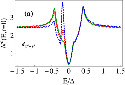
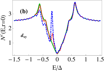
Figure 4: (color online) LDOS for the superconducting regime with order parameters: a) d${}_{x^{2}-y^{2}}$ and b) d_xy; for $\epsilon_{f}=-\Delta_{0}/3$, $V_{1}=V_{2}=0$ (green), $V_{1}=V_{2}=0.5\Delta_{0}$ (red), and $V_{1}=V_{2}=\Delta_{0}$ (blue).

III Numerical results

We now discuss the results of numerical calculations for the central quantity $N^{c}(E,{\bf r})$ based on the previous analysis (obtained from Eqs. 11-17). In this section we focus on the energy and also spatial dependence of the local density of states (LDOS) (Eq. 5) at $T=0$ for various gap symmetries. As the main candidates we include different types of the extended s-wave gaps which are fully gapped on the hole pocket but possibly have accidental nodes on the electron pockets due to higher harmonics contributions. For completeness, we also include d-wave gap functions which have nodes on both electron and hole pockets. The latter however are not supported by ARPES results Ding08 ; Kondo08 ; Lue09 which suggest nodeless gaps on the hole pockets.

We begin our discussion with the anisotropic nodeless extended s-wave pairing function (S^±). The Fermi surface illustration with respective node positions indicated by dashed lines is shown in Fig.1.(a). This gap function is given by

$$\Delta_{S^{\pm}}(k_{x},k_{y})=\frac{\Delta_{0}}{2}(\cos k_{x}+\cos k_{y}),$$ (18)

and we show the result for the LDOS at the origin $(r_{x},r_{y})=(0,0)$ in Fig.2(a) for $\Delta_{0}=6$ meV and $\epsilon_{f}=-\Delta_{0}/3$, with different hybridization energies $V_{1}=V_{2}=0$ (green), $V_{1}=V_{2}=0.5\Delta_{0}$ (red), and $V_{1}=V_{2}=\Delta_{0}$ (blue). While the overall structure of the spectrum stays the same the increased hybridization leads to more pronounced bound state peaks within the gap. We observe that an increase of the hybridization energy, $V_{\gamma}$, causes the position of peaks to move to higher absolute values of $E$, and a corresponding increase of their line width. By increasing the absolute value of the impurity energy level, $\epsilon_{f}$ , the bound state also moves to higher absolute values of $E$. Notice that by restricting to the first order perturbation theory in effective hybridization (Born approximation), we did not find a dramatic change in our results, for the chosen values of $V_{\gamma}$.

Furthermore, due to the different size of electron and hole pockets the onset of the continuum around $|E/\Delta|$ is split into a double peak structure. For $E>0$ the lower and upper peaks correspond to hole and electron pockets, respectively.

The addition of higher harmonics in the S${}_{1}^{\pm}$ gap function allows to tune the modulus of the gaps on hole and electron pockets independently while keeping the basic property of having an opposite signs. As seen from Fig.1(a) this is equivalent to shift of the nodal line position closer to the electron pockets and increasing higher harmonic amplitude continuously one eventually produce an accidental node on this sheet. This gap function is given by

$$\Delta_{S_{1}^{\pm}}(k_{x},k_{y})=$$

$$\Delta_{0}\left[\frac{1}{2}(\cos k_{x}+\cos k_{y})+\alpha\cos\frac{k_{x}}{2}\cos\frac{k_{y}}{2}\right],$$ (19)

and the result for the LDOS is plotted in Fig.(2(b)-(f) for different $\alpha$ parameters. At the symmetry points one has $\Delta_{(0,0)}=\Delta_{0}(1+\alpha)$ and $\Delta_{(\pi,\pi))}=-\Delta_{0}$. Then $|\Delta_{(0,0)}|-|\Delta_{(\pi,\pi))}|=\alpha$ which also means that the difference between the absolute values of the gaps on $\Gamma$-centered hole pockets and M-centered electron pockets increases with $\alpha$. This can be clearly seen in Fig. 2(b) ($\alpha=1$) where the peak at larger $|E/\Delta_{0}|$ originating from the hole pocket is pushed to larger energies and for $\alpha=3$ is no longer visible on the scale of Fig. 2(c). On the other hand the peak due to gap maximum on the electron pocket stays fixed around $|E/\Delta_{0}|\simeq 1$ while $\alpha$ grows. At the same time a deep minimum and finally an accidental node of the gap develops on the electron pocket and leads to the increase of the low energy LDOS in Figs.2(b)-(f). This type of low energy DOS may explain power laws for NMR relaxation rate and penetration depth observed in some pnictidesNakai08 ; Shan08 ; Mu08 . On the other hand the position of bound state peaks caused by the magnetic impurity is apparently insensitive to the variation of $\alpha$ and the change of the underlying quasiparticle spectrum.

However, the S${}_{1}^{\pm}$ gap function is not unique and accidental nodes on the electron pocket may be obtained with a different type of modification with higher harmonics. This leads us to extended S${}_{2}^{\pm}$-wave pairing described by another gap function

$$\Delta_{S_{2}^{\pm}}(k_{x},k_{y})=\Delta_{0}\left[0.5(\cos k_{x}+\cos k_{y})\right.$$

$$\left.+\alpha\cos k_{x}\cos k_{y}+\alpha^{\prime}\cos 4k_{x}\cos 4k_{y}\right].$$ (20)

Its nodal structure is shown in (Fig. 1(b). Now there are two nodal lines, one located between the pockets which leads to an anisotropic but fully gapped order parameter on the hole pockets. The other accidental nodal line centered around the M point cuts the electron pocket and leads to a finite low energy quasiparticle DOS as seen in the results of the Figs.(3(a) and 3(b) for $\alpha=1.2;\;\alpha^{\prime}=0.15$ and $\alpha=1.17;\;\alpha^{\prime}=0.08$ respectively. The bound states due to impurity scattering appear again as pairs at similar energies as for the S${}_{1}^{\pm}$ case.

Finally for completeness we also consider two simple anisotropic d-wave order parameters, namely d${}_{x^{2}-y^{2}}$ (Fig. 1(d)) and d_xy (Fig. 1(e)) which have symmetry enforced gap nodes. This leads to sign change of the gap function on the same FS pocket rather than between them. We consider the two candidates

$$\Delta_{d_{x^{2}-y^{2}}}(k_{x},k_{y}) = \frac{\Delta_{0}}{2}\left(\cos k_{x}-\cos k_{y}\right),$$

$$\Delta_{d_{xy}}(k_{x},k_{y}) = \Delta_{0}\sin k_{x}\sin k_{y}.$$ (21)

In each case the nodal lines cross both Fermi surface pockets in contrast to the extended s-wave model. We note that current ARPES experiments have shown a fully gapped hole pocket Ding08 ; Kondo08 ; Lue09 though no experiments yet are available for $P$-based systems.

The background of the LDOS is given by the typical V-shape of a d-wave order parameter. On top of it a single bound state peak due to the impurity scattering appears below the Fermi level. This is distinctly different from the extended s-wave case where always two bound states below and above the Fermi level appear symmetrically. A partly similar observation for a d${}_{x^{2}-y^{2}}$ order parameter with only a single sheet FS intended for cuprates was made in Ref. Zhang01, . There one bound state peak was found for $(r_{x},r_{y})$ along the anti-nodal direction and two peaks for the nodal direction. In our present d-wave case considered for the two-sheet FS of Fe pnictides the single peak appears for both nodal and anti-nodal directions.

For clarifying of the position dependence of resonance peaks, Fig.5 displays the spatial variation of the LDOS $N_{c}(\omega,r_{x},r_{y})$ around the magnetic impurity at the resonance energies, (a) $\omega=\omega_{r}$ and (b) $\omega=-\omega_{r}$, for S^± gap symmetry with $\Delta_{0}=6$meV; $\epsilon_{f}=-\Delta_{0}/3$, and $V_{1}=V_{2}=\Delta_{0}$. It shows that the maximum amplitude of the LDOS appears close to the impurity site and decays non-monotonically further away from the impurity site. While the LDOS at $\omega_{r}$ is rather isotropic the peak for $-\omega_{r}$ shows a significant anisotropic LDOS in the plane. This anisotropy does not seem to result from special FeAs Fermi surface feature since it is also observed in the single parabolic band case in Ref. Zhang01, .

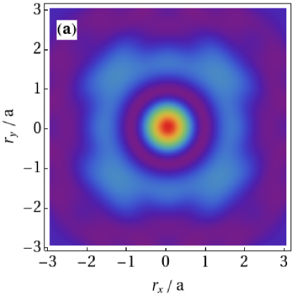
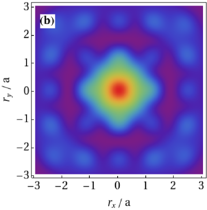
Figure 5: (color online) Density plot of the spatial distribution of the LDOS for the superconducting regime with extended s-wave order parameter, $\Delta_{S^{\pm}}(k_{x},k_{y})$, for $\epsilon_{f}=-\Delta_{0}/3$, $V_{1}=V_{2}=\Delta_{0}$, and a) $\omega=\omega_{r}$, b) $\omega=-\omega_{r}$. (Red color correspond to large LDOS).

IV Summary

We have investigated the effect of magnetic impurity scattering in the FeAs pnictide superconductors. We used a simple two band model Fermi surface and calculated LDOS spectral and spatial dependence close to the impurity site for two types of extended s-wave superconducting order parameters with inter-band sign change and for two d-wave order parameters with intra-band sign change. In the former two impurity bound states appear symmetrically around the Fermi energy at positions $\pm\omega_{r}$. The modulus of the bound state energy increases with hybridization strength $V$ and impurity orbital energy $\epsilon_{f}$ monotonically. In the latter case only the lower bound state pole at $-\omega_{r}$ appears in the LDOS for any direction from the impurity site. The background variation of the LDOS is determined by the characteristics of the superconducting gap on the two FS sheets. The extended S-wave order parameters may be tuned such that fully gapped behavior on the central hole sheet and accidental node structure on the zone boundary hole sheets appear naturally. In this case the spatial dependence of the LDOS for the two bound state peaks shows significant differences in the degree of spatial anisotropy. We conclude that the observation of two bound state peaks in tunneling experiments would be an important support for the extended s-wave gap function with interband sign change. The fine structure of the background continuum LDOS may give more detailed information on the type of the accidental nodal structure.

References

- (1) H. Shiba, Prog. Theor. Phys. 40, 435 (1968).
- (2) M. Matsumoto, and M. Koga, J. Phys. Soc. Jpn. 71S, 231 (2002).
- (3) O. Sakai, Y. Shimizu, K. Satori, and H. Shiba, J. Phys. Soc. Jpn. 62, 3181 (1993).
- (4) K. Satori, H. Shiba, O. Sakai and Y. Shimizu, J. Phys. Soc. Jpn. 61, 3239 (1992).
- (5) A. V. Balatsky, I. Vekhter and J.-X. Zhu, Rev. Mod. Phys. 78, 373 (2006).
- (6) Y. Kamihara, T. Watanabe, M. Hirano and H. Hosono, J. Am. Chem. Soc. 130, 3296 (2008 ).
- (7) E.M. Brüning, C. Krellner, M. Baenitz, A. Jesche, F. Steglich, and C. Geibel, Phy. Rev. Lett. 101, 117206 (2008).
- (8) J. Zhao, Q. Huang, C. de la Cruz, S. Li, J.W. Lynn, Y. Chen, M.A. Green, G.F. Chen, G. Li, Z.C. Li, J.L. Luo, N.L. Wang, and P. Dai, Nat. Mat. 7, 953 (2008).
- (9) L. Pourovskii, V. Vildosola, S. Biermann and A. Georges, Europhys. Lett. 84, 37006 (2008).
- (10) K. Kuroki, S. Onari, R. Arita, H. Usui, Y. Tanaka, H. Kontani and H. Aoki, Phys. Rev. Lett. 101, 087004 (2008).
- (11) T. A. Maier, S. Graser, D.J. Scalapino, and P. J. Hirschfeld, Phys. Rev. B 79, 224510 (2009).
- (12) J. Zhang, R. Sknepnek, R. M. Fernandes and J. Schmalian,Phys. Rev. B 79, 220502(R) (2009).
- (13) A. V. Chubukov, D. V. Efremov and I. Eremin, Phys. Rev. B 78, 134512 (2008).
- (14) H. Zhai, Fa Wang and Dung-Hai Lee, Phys. Rev. B 80, 064517 (2009).
- (15) H. Luetkens, H.-H. Klauss, M. Kraken, F. J. Litterst, T. Dellmann, R. Klingeler, C. Hess, R. Khasanov, A. Amato, C. Baines, M. Kosmala, O. J. Schumann, M. Braden, J. Hamann-Borrero, N. Leps, A. Kondrat, G. Behr, J. Werner and B. Büchner, Nature Materials 8, 305-309 (2009).
- (16) K. Hashimoto, M. Yamashita, S. Kasahara, Y. Senshu, N. Nakata, S. Tonegawa, K. Ikada, A. Serafin, A. Carrington, T. Terashima, H. Ikeda, T. Shibauchi, Y. Matsuda, arXiv:0907.4399(unpublished).
- (17) L. Malone, J.D. Fletcher, A. Serafin, A. Carrington, N.D. Zhigadlo, Z. Bukowski, S. Katrych, J. Karpinski, Phys. Rev. B 79, 140501(R) (2009).
- (18) R. Khasanov, H. Luetkens, A. Amato, H. H. Klauss, Z. A. Ren, J. Yang, W. Lu, Z. X. Zhao, Phys. Rev. B 78, 092506 (2008).
- (19) G. M. Zhang, H. Hu, and L. Yu, Phys. Rev. Lett. 86, 704 (2001).
- (20) Y. Nakai, K. Ishida, Y. Kamihara, M. Hirano and H. Hosono, J. Phys. Soc. Japan, 77, 073701 (2008).
- (21) L. Shan, Y. Wang, X. Zhu, G. Mu, L. Fang, C. Ren, H. Wen, Europhysics Letters, 83, 57004 (2008).
- (22) G. Mu, Z. Xi-Yu, F. Lei, S. Lei, R. Cong and W. Hai-Hu, Chin. Phys. Lett. 25, 2221 (2008).
- (23) A.V. Chubukov, M.G. Vavilov, A.B. Vorontsov, Phys. Rev. B 80, 140515(R) (2009).
- (24) A. Moreo, M. Daghofer, A. Nicholson, E. Dagotto, Phys. Rev. B 80, 104507 (2009).
- (25) K. Kuroki, H. Usui, S. Onari, R. Arita, and H. Aoki, Phys. Rev. B 79, 224511 (2009).
- (26) M. Matsumoto, M. Koga and H. Kusunose, J. Phys. Soc. Jpn. 78, 084718 (2009).
- (27) D. Zhang, T. Zhou and C. S. Ting, arXiv:0904.3708 (unpublished).
- (28) W. F. Tsai, Y. Y. Zhang, C. Fang, and J. Hu, Phys. Rev. B80, 064513 (2009).
- (29) E.W. Hudson, K.M. Lang, V. Madhavan, S.H. Pan, H. Eisaki, S. Uchida, and J.C. Davis, Nature 411, 920 (2001).
- (30) Y. Senga and H. Kontani, J. Phys. Soc. Jpn. 77, 113710 (2008).
- (31) S. Onari and H. Kontani, Phys. Rev. Lett. 103, 177001 (2009).
- (32) J. Li and Y. Wang, Europhysics Letters, 88 17009 (2009).
- (33) D.J. Singh and M.-H. Du, Phys. Rev. Lett. 100, 237003 (2008); L. Boeri, O.V. Dolgov, and A.A. Golubov, Phys. Rev. Lett. 101, 026403 (2008); I.I. Mazin, D.J. Singh, M.D. Johannes, and M.H. Du, Phys. Rev. Lett. 101, 057003 (2008).
- (34) C. Liu, G.D. Samolyuk, Y. Lee, N. Ni, T. Kondo, A.F. Santander-Syro, S.L. Bud’ko, J.L. McChesney, E. Rotenberg, T. Valla, A. V. Fedorov, P.C. Canfield, B.N. Harmon, A. Kaminski, Phys. Rev. Lett. 101, 177005 (2008); D.V. Evtushinsky, D.S. Inosov, V.B. Zabolotnyy, A. Koitzsch, M. Knupfer, B. Büchner, M. S. Viazovska,G.L. Sun, V. Hinkov, A.V. Boris, C.T. Lin, B. Keimer, A. Varykhalov, A.A. Kordyuk, and S.V. Borisenko, Phys. Rev. B 79, 054517 (2009); D. Hsieh, Y. Xia, L. Wray, D. Qian, K. Gomes, A. Yazdani, G.F. Chen, J.L. Luo, N.L. Wang, and M.Z. Hasan, arXiv:0812.2289 (unpublished); H. Ding, K. Nakayama, P. Richard, S. Souma, T. Sato, T. Takahashi, M. Neupane, Y.-M. Xu, Z. H. Pan, A.V. Federov, Z. Wang, X. Dai, Z. Fang, G.F. Chen, J.L. Luo, N.L. Wang, arXiv:0812.0534 (unpublished).
- (35) M.M. Korshunov and I. Eremin, Phys. Rev. B 78, 140509(R) (2008).
- (36) K. Nakayama, T. Sato, P. Richard, T. Kawahara, Y. Sekiba, T. Qian, G. F. Chen, J. L. Luo, N. L. Wang, H. Ding, T. Takahashi, arXiv:0907.0763 (unpublished).
- (37) P. Coleman. Phys. Rev. B 29 3035 (1984).
- (38) H. Ding, P. Richard, K. Nakayama, K. Sugawara, T. Arakane, Y. Sekiba, A. Takayama, S. Souma, T. Sato, T. Takahashi, Z. Wang, X. Dai, Z. Fang, G. F. Chen, J. L. Luo and N. L. Wang, Europhys. Lett. 83, 47001 (2008).
- (39) T. Kondo, A. F. Santander-Syro, O. Copie, C. Liu, M. E. Tillman, E. D. Mun, J. Schmalian, S. L. Budko, M. A. Tanatar, P. C. Canfield, and A. Kaminski, Phys. Rev. Lett. 101, 147003 (2008).