On the nonperturbative solution of Pauli–Villars-regulated light-front QED:
A comparison of the sector-dependent and standard parameterizations

Abstract

We consider quantum electrodynamics quantized on the light front in Feynman gauge and regulated in the ultraviolet by the inclusion of massive, negative-metric Pauli–Villars (PV) particles in the Lagrangian. The eigenstate of the electron is approximated by a Fock-state expansion truncated to include one photon. The Fock-state wave functions are computed from the fundamental Hamiltonian eigenvalue problem and used to calculate the anomalous magnetic moment, as a point of comparison. Two approaches are considered: a sector-dependent parameterization, where the bare parameters of the Lagrangian are allowed to depend on the Fock sectors between which the particular Hamiltonian term acts, and the standard choice, where the bare parameters are the same for all sectors. Both methods are shown to require some care with respect to ultraviolet divergences; neither method can allow all PV masses to be taken to infinity. In addition, the sector-dependent approach suffers from an infrared divergence that requires a nonzero photon mass; due to complications associated with this divergence, the standard parameterization is to be preferred. We also show that the self-energy effects obtained from a two-photon truncation are enough to bring the standard-parameterization result for the anomalous moment into agreement with experiment within numerical errors. This continues the development of a method for the nonperturbative solution of strongly coupled theories, in particular quantum chromodynamics.

1 Introduction

The nonperturbative solution of quantum field theories has proven to be a difficult task. The method that has had the most success to date, lattice gauge theory [1], has attained this success only after a long period of development, with a great number of technical innovations along the way. What is more, the level of success that can be achieved is inherently limited by the lack of direct contact with wave functions for bound-state constituents and by the Euclidean formulation. The limitation of Euclidean formulation is shared by the method of Dyson–Schwinger equations [2], which are coupled equations for the $n$-point Euclidean Green’s functions where bound states appear as poles in the propagators. Solution of the infinite system requires truncation and a model for the highest $n$-point functions.

In order to calculate wave functions directly in a Minkowskian formulation, there has been an effort for a number of years to develop a Hamiltonian approach in light-cone quantization [3]. Although the ultimate objective is to be able to solve for the bound states of QCD, most of the development has been in QED and simpler theories, such as Yukawa theory and $\phi^{4}$ theory. Many two-dimensional theories have been solved; however, success with four-dimensional theories has been limited by the need for a consistent regularization and renormalization scheme and by the large size of the numerical calculation. There is also a related light-front lattice Hamiltonian formulation, known as the transverse lattice method [4], which we do not consider here.

A regularization scheme that has been useful in doing perturbative light-cone calculations is the alternate denominator method of Brodsky, Roskies, and Suaya [5]. Because of its success, one would naturally consider extending this approach to nonperturbative calculations. Unfortunately, application of the method requires explicit identification of light-cone energy denominators, which are only implicit in the coupled equations of the nonperturbative mass eigenvalue problem. One could instead use the alternate denominator method to construct counterterms, and then incorporate the counterterms in the Hamiltonian for the nonperturbative calculation. However, these counterterms would be limited to a particular order in the coupling while the nonperturbative problem sums a partial set of contributions to all orders. Instead, one needs a method that generates counterterms to all orders, but no more than what is needed.

A method for regularization that has proven quite useful is Pauli–Villars (PV) regularization [6], which was developed and tested in a series of calculations [7, 8, 9, 10, 11, 12, 13, 14]. The key idea is to include enough PV fields in the Lagrangian to regulate the theory perturbatively and, where possible, maintain symmetries. The derived light-front Hamiltonian then defines the nonperturbative bound-state problem. As for the eigenstate, it is approximated by a truncated Fock-state expansion. Then the mass eigenvalue problem leads to coupled integral equations for the Fock-state wave functions. The PV particles appear in the Fock states and, through chosen negative metrics, bring about the subtractions necessary to regulate the integral equations. A possible formulation for QCD along these lines has been given by Paston et al. [16].

Two methods of parameterization are in use. One is the standard choice, where the bare parameters are those of the regulated Lagrangian. The other is a sector-dependent parameterization [17], where the bare parameters are allowed to depend on the Fock sector(s) on which the Hamiltonian acts. In either case, the parameters are fixed by constraints from observables and from symmetry restorations. The standard scheme has been used extensively in studies of PV regularization [7, 8, 9, 10, 11, 12, 13, 14]. The sector-dependent scheme was first systematically applied to QED by Hiller and Brodsky [18], though they did not consider a sector-dependent vertex mass. More recently, it was investigated by Karmanov, Mathiot, and Smirnov [19]. In order to better understand how to proceed with the large-scale numerical calculations that need to be done, a comparison of these approaches needs to be made.

Both parameterizations require some care, particularly with respect to uncanceled divergences. In the standard method, an uncanceled divergence appears in the following way [12]. The results for a generic physical quantity, such as the electron’s anomalous moment, will be of the form

$$\lim_{\mu_{\rm PV}\rightarrow\infty}g^{2}\frac{a_{1}\,[+a_{2}g^{2}\ln\mu_{\rm PV}+\cdots]}{1+b_{1}g^{2}+b_{2}g^{2}\ln\mu_{\rm PV}+\cdots}=\left\{\begin{array}[]{ll}0,&\mbox{with truncation}\\ \mbox{finite},&\mbox{without truncation},\end{array}\right.$$ (1)

where $\mu_{\rm PV}$ is a PV mass scale and the contents of the square brackets are absent in the case of truncation. When the limit $\mu_{\rm PV}\rightarrow\infty$ is taken, the result is either zero or a finite value. As the PV mass $\mu_{\rm PV}$ is increased, the divergence in the denominator is not canceled by a divergence in the numerator, if the truncation is made. Therefore, any potentially meaningful calculation must be done at finite $\mu_{\rm PV}$, in a range of scales where the errors due to truncation and PV inclusion are minimized.

The sector-dependent method is also limited to finite PV mass scales by an uncanceled divergence. As shown in [18], the bare coupling can become imaginary if the PV masses become too large. Also, as we will show below, the probabilities for individual Fock sectors are driven outside the range of 0 to 1. The authors of [19] do not consider these limitations and calculate quantities that do not depend directly on this bare coupling; they then have a result at infinite PV masses, but the underlying theory and its wave functions are ill defined.

Instead, the calculation should be done at finite PV masses. Here we do this, for the anomalous magnetic moment of the electron computed in the one-photon truncation of the dressed-electron state, and compare the results of the standard [14] and sector-dependent [19] approaches. In this particular context, the dressed electron can be viewed as a bound state of bare constituents, electron and photon, in QED. The particular truncation is chosen because the eigenvalue problem can be solved analytically and the comparison is not obscured by numerical artifacts. The calculation of the anomalous moment is not intended as competitive with perturbation theory [20]; the weak coupling of QED makes nonperturbative calculations much less accurate. However, the calculation does stand as a test of a method that can be applied where perturbation theory is useless.

Convergence with respect to the Fock-state expansion has been checked in Yukawa theory [9]. There a full discrete light-cone quantization (DLCQ) [21] calculation was possible. The DLCQ approach does truncate the Fock-state expansion but only to the extent required by the numerical resolution; more constituents are allowed as the discrete momentum fraction is reduced. Explicit truncations to fewer constituents can be made and the results compared. For Yukawa theory, the comparison showed that the Fock-state expansion converges quickly.

The analogous results for a cubic scalar theory [22] do not show such rapid convergence. However, this is because the spectrum of the theory is unbounded from below [23], and the lowest eigenstates are dominated by Fock states with large numbers of constituents [24]. In other words, for cubic scalar theories the highest Fock states make the largest contributions. Yukawa theory and QED do not suffer this fate because of the Pauli principle.

In order to have a simple vacuum and a well-defined Fock-state expansion, we use light-cone coordinates [25, 3] $\underline{x}=(x^{-}=t-z,\vec{x}_{\perp}=(x,y))$ and light-cone momenta $\underline{p}=(p^{+}=p^{0}+p^{z},\vec{p}_{\perp})$. The light-cone energy $p^{-}=p^{0}-p^{z}$ is conjugate to the light-cone time $x^{+}=t+z$. Stationary states are obtained as eigenstates of the light-cone Hamiltonian [3] ${\cal P}^{-}$, which defines the mass eigenvalue problem ${\cal P}^{-}|P\rangle=\frac{M^{2}}{P^{+}}|P\rangle$, in a frame where the total transverse momentum $\vec{P}_{\perp}$ is zero. Further details of the coordinate choice can be found in [14] or [3].

To further develop the method in the context of a gauge theory, we consider QED. To regulate QED, we use one PV electron and two PV photons. The second PV photon is needed to restore chiral symmetry in the massless-electron limit [14]. The couplings and metrics of the PV fields are adjusted to accomplish the ultraviolet regularization and the finite chiral-symmetry correction. They also provide for cancellation of instantaneous fermion interactions and allow the constraint equation for the nondynamical fermion fields to be solved exactly without use of light-cone gauge [14].

In Sec. 2 of [12], there is some discussion of the use of three PV fermions to regulate QED. However, this was included only to show that naive PV regularizations in light-cone gauge do not necessarily work. A regularization in light-cone gauge that does work is given in Sec. 4 of that paper, but this requires additional regulators that complicate the theory. The simplest regularization, which uses one PV fermion and one PV boson, is found for Feynman gauge and discussed in Sec. 3. There the chiral limit is correct, but only because the PV electron mass is taken to infinity. If the PV electron mass is kept finite, regularization by one PV photon is insufficient for both standard and sector-dependent parameterizations.

Also, the result in [12] for the anomalous moment of the electron differs from the Schwinger result [26]. The source of the difference is not the uncanceled divergence. Instead, it is contributions from all higher orders in the coupling constant, consistent with the Fock-space truncation to one electron and one photon. The effect of the uncanceled divergence, which appears in the denominators of Fock-state probabilities, is logarithmic and quite mild, and, in any case, can only make the estimate for the anomalous moment smaller than the Schwinger result. The estimate obtained is instead larger, due to sensitivity to the constituent (bare) electron and photon masses and the nonperturbative shift of the constituent electron mass. Here we correct this shift by including the self-energy contribution from the one-electron/two-photon sector and find very good agreement with experiment.

The sector-dependent approach, as used in [19], does no better than lowest-order perturbation theory, which is quite strange, since a nonperturbative calculation should include some physics to all orders. In addition, the calculation in [19] suffers from uncanceled divergences that appear in the numerators of Fock-state probabilities, instead of the denominators, and that push these probabilities outside the physical range of $[0,1]$.

With this as introduction, we continue in Sec. 2 with a comparison of the standard and sector-dependent parameterizations in a one-photon truncation of the Fock expansion for the dressed electron. In Sec. 3, the standard-parameterization results are extended to include self-energy contributions that correspond to intermediate states with two photons. Section 4 contains a summary of the comparison and some general discussion of applications. A provides specifics about light-front QED in Feynman gauge, with further details available in [12] and [14]. B gives details of the solution when self-energy contributions are included.

2 One-Photon Truncation

We work in Feynman-gauge QED quantized on the light-front and regulated with one PV electron and two PV photons. Details are given in A.

2.1 Fock-State Expansion

We seek the solution for the dressed-electron eigenstate truncated to include only the bare-electron and one-electron/one-photon Fock sectors. The Fock-state expansion for the eigenstate with total $J_{z}=\pm\frac{1}{2}$ is then

$$|\psi^{\pm}(\underline{P})\rangle=\sum_{i}z_{i}b_{i\pm}^{\dagger}(\underline{P})|0\rangle+\sum_{ijs\mu}\int d\underline{k}C_{ijs}^{\mu\pm}(\underline{k})b_{is}^{\dagger}(\underline{P}-\underline{k})a_{j\mu}^{\dagger}(\underline{k})|0\rangle.$$ (2)

The amplitudes $z_{i}$ and wave functions $C_{ijs}^{\mu\pm}$ define this state.

The interpretation of the expansion requires projection onto a physical subspace. We apply the same approach as was used in Yukawa theory [11], where a projection onto the physical subspace is accomplished by expressing Fock states in terms of positively normed creation operators and null combinations. Here, the positive-norm operators are $a_{0\mu}^{\dagger}$, $a_{2\mu}^{\dagger}$, and $b_{0s}^{\dagger}$, and the null combinations are $a_{\mu}^{\dagger}=\sum_{i}\sqrt{\xi_{i}}a_{i\mu}^{\dagger}$ and $b_{s}^{\dagger}=b_{0s}^{\dagger}+b_{1s}^{\dagger}$. The $b_{s}^{\dagger}$ particles are annihilated by the generalized electromagnetic current $\bar{\psi}\gamma^{\mu}\psi$; thus, $b_{s}^{\dagger}$ creates unphysical contributions to be dropped, and, by analogy, we also drop contributions created by $a_{\mu}^{\dagger}$. The projected dressed-fermion state is

$$|\psi_{\rm phys}^{\pm}(\underline{P})\rangle=\sum_{i}(-1)^{i}z_{i}b_{0\pm}^{\dagger}(\underline{P})|0\rangle$$

$$+\sum_{s\mu}\int d\underline{k}\sum_{i=0}^{1}\sum_{j=0,2}\sqrt{\xi_{j}}\sum_{k=j/2}^{j/2+1}\frac{(-1)^{i+k}}{\sqrt{\xi_{k}}}C_{iks}^{\mu\pm}(\underline{k})b_{0s}^{\dagger}(\underline{P}-\underline{k})a_{j\mu}^{\dagger}(\underline{k})|0\rangle.$$

The normalization condition

$$\langle\psi_{\rm phys}^{\sigma^{\prime}}(\underline{P}^{\prime})|\psi_{\rm phys}^{\sigma}(\underline{P})\rangle=\delta(\underline{P}^{\prime}-\underline{P})\delta_{\sigma^{\prime}\sigma}$$ (4)

is then applied.

The projection is critical, not only for the removal of negatively normed contributions which could make probabilistic interpretations difficult, but also for the regularization of expectation values. In particular, a calculation of the expectation value of the number of photons in the dressed-electron state will yield infinity for the unprojected Fock expansion, because the spin-flip wave function $C_{ij\mp}^{\mu\pm}(\underline{k})$ falls off inversely with $k_{\perp}$. The projection introduces subtractions that remove this divergent behavior. In [19], such a projection is not made and instead the eigenstate is to be interpreted only as part of a larger process; the associated Fock-state wave functions have no direct utility.

2.2 Coupled Equations

Our Fock-space-truncated eigenstate has to satisfy the mass-squared eigenvalue problem ${\cal P}^{-}|\psi\rangle=\frac{M^{2}}{P^{+}}|\psi\rangle$. Projections onto each Fock sector yield coupled equations for the one-photon amplitudes $z_{i}$ and one-electron/one-photon wave functions $C_{ijs}^{\mu\pm}$. These coupled equations are, with $y=k^{+}/P^{+}$,

$$[M^{2}-m_{i}^{2}]z_{i} = \int(P^{+})^{2}dyd^{2}k_{\perp}\sum_{j,l,\mu}\sqrt{\xi_{l}}(-1)^{j+l}\epsilon^{\mu}$$

$$\times\left[V_{ji\pm}^{\mu*}(\underline{P}-\underline{k},\underline{P})C^{\mu\pm}_{jl\pm}(\underline{k})+U_{ji\pm}^{\mu*}(\underline{P}-\underline{k},\underline{P})C^{\mu\pm}_{jl\mp}(\underline{k})\right],$$

and

$$\left[M^{2}-\frac{m_{j}^{2}+k_{\perp}^{2}}{1-y}-\frac{\mu_{l}^{2}+k_{\perp}^{2}}{y}\right]C^{\mu\pm}_{jl\pm}(\underline{k})=\sqrt{\xi_{l}}\sum_{i^{\prime}}(-1)^{i^{\prime}}z_{i^{\prime}}P^{+}V_{ji^{\prime}\pm}^{\mu}(\underline{P}-\underline{k},\underline{P}),$$ (6)

$$\left[M^{2}-\frac{m_{j}^{2}+k_{\perp}^{2}}{1-y}-\frac{\mu_{l}^{2}+k_{\perp}^{2}}{y}\right]C^{\mu\pm}_{jl\mp}(\underline{k})=\sqrt{\xi_{l}}\sum_{i^{\prime}}(-1)^{i^{\prime}}z_{i^{\prime}}P^{+}U_{ji^{\prime}\pm}^{\mu}(\underline{P}-\underline{k},\underline{P}).$$ (7)

The indices are arranged such that an index of $i$ corresponds to the one-electron sector and $j$ to the one-electron/one-photon sector. Therefore, in the sector-dependent approach, a mass $m_{i}$ in a vertex function is assigned the bare mass, and $m_{j}$ is the physical mass. In the standard parameterization, all are bare masses.

The coupled equations can be solved analytically [12]. The wave functions $C_{ils}^{\mu\pm}$ are

$$C^{\mu\pm}_{il\pm}(\underline{k}) = \sqrt{\xi_{l}}\frac{\sum_{j}(-1)^{j}z_{j}P^{+}V_{ij\pm}^{\mu}(\underline{P}-\underline{k},\underline{P})}{M^{2}-\frac{m_{i}^{2}+k_{\perp}^{2}}{1-y}-\frac{\mu_{l}^{2}+k_{\perp}^{2}}{y}},$$ (8)

$$C^{\mu\pm}_{il\mp}(\underline{k}) = \sqrt{\xi_{l}}\frac{\sum_{j}(-1)^{j}z_{j}P^{+}U_{ij\pm}^{\mu}(\underline{P}-\underline{k},\underline{P})}{M^{2}-\frac{m_{i}^{2}+k_{\perp}^{2}}{1-y}-\frac{\mu_{l}^{2}+k_{\perp}^{2}}{y}},$$ (9)

and the amplitudes satisfy

$$(M^{2}-m_{i}^{2})z_{i}=2e_{0}^{2}\sum_{i^{\prime}}(-1)^{i^{\prime}}z_{i^{\prime}}\left[\bar{J}+m_{i}m_{i^{\prime}}\bar{I}_{0}-2(m_{i}+m_{i^{\prime}})\bar{I}_{1}\right],$$ (10)

with [12]

$$\bar{I}_{n}(M^{2}) = \int\frac{dydk_{\perp}^{2}}{16\pi^{2}}\sum_{jl}\frac{(-1)^{j+l}\xi_{l}}{M^{2}-\frac{m_{j}^{2}+k_{\perp}^{2}}{1-y}-\frac{\mu_{l}^{2}+k_{\perp}^{2}}{y}}\frac{m_{j}^{n}}{y(1-y)^{n}}\,,$$ (11)

$$\bar{J}(M^{2}) = \int\frac{dydk_{\perp}^{2}}{16\pi^{2}}\sum_{jl}\frac{(-1)^{j+l}\xi_{l}}{M^{2}-\frac{m_{j}^{2}+k_{\perp}^{2}}{1-y}-\frac{\mu_{l}^{2}+k_{\perp}^{2}}{y}}\frac{m_{j}^{2}+k_{\perp}^{2}}{y(1-y)^{2}}.$$ (12)

Each integral can be computed analytically. For the sector-dependent parameterization, the convention of $m_{i}$ being a bare mass and $m_{j}$ a physical mass has been maintained, with the extension that $m_{i^{\prime}}$ is also a bare mass. The integrals $\bar{I}_{n}$ and $\bar{J}$ then depend only on the physical mass, and (10) is equivalent to perturbation theory. For the standard parameterization, $\bar{I}_{n}$ and $\bar{J}$ depend on the bare mass, and (10) is nonperturbative.

With use of the identity [14] $\bar{J}=M^{2}\bar{I}_{0}$, $\bar{J}$ can be eliminated from the eigenvalue problem. This allows the solution to the eigenvalue problem (10) to take the simple form [12]

$$\alpha_{0\pm}=\frac{(M\pm m_{0})(M\pm m_{1})}{8\pi(m_{1}-m_{0})(2\bar{I}_{1}\pm M\bar{I}_{0})},\;\;z_{1}=\frac{M\pm m_{0}}{M\pm m_{1}}z_{0},$$ (13)

with $\alpha_{0}=e_{0}^{2}/4\pi$ and $z_{0}$ determined by the normalization (4), which reduces to

$$1 = (z_{0}-z_{1})^{2}$$

$$+\frac{\alpha_{0}}{2\pi}\int ydydk_{\perp}^{2}\sum_{l,l^{\prime}}(-1)^{l+l^{\prime}}z_{l}z_{l^{\prime}}\sum_{i^{\prime}i}(-1)^{i^{\prime}+i}\sum_{j=0,2}\xi_{j}$$

$$\sum_{k^{\prime}=j/2}^{j/2+1}\sum_{k=j/2}^{j/2+1}\frac{(-1)^{k^{\prime}+k}}{[ym_{i^{\prime}}^{2}+(1-y)\mu_{k^{\prime}}^{2}+k_{\perp}^{2}-m_{e}^{2}y(1-y)]}$$

$$\times\frac{m_{i^{\prime}}m_{i}-(m_{i}+m_{i^{\prime}})(m_{l}+m_{l^{\prime}})(1-y)+m_{l}m_{l^{\prime}}(1-y)^{2}+k_{\perp}^{2}}{[ym_{i}^{2}+(1-y)\mu_{k}^{2}+k_{\perp}^{2}-m_{e}^{2}y(1-y)]}.$$

2.3 Discussion of the Solution

Since the PV fermion is needed only to regulate the integral $\bar{J}$, which has been eliminated from the calculation, we can safely take the $m_{1}\rightarrow\infty$ limit, to simplify the remaining steps. In this limit, we have $z_{1}=0$, $m_{1}z_{1}\rightarrow\pm(M-m_{0})z_{0}$, and

$$\alpha_{0\pm}=\pm\frac{M(M\pm m_{0})}{8\pi(2\bar{I}_{1}\pm M\bar{I}_{0})}.$$ (15)

Also, the third constraint (54) is automatically satisfied, and the second PV photon flavor can be discarded.

For the standard parameterization, we cannot solve explicitly for $m_{0}$, because $\bar{I}_{0}$ and $\bar{I}_{1}$ are functions of $m_{0}$. However, $\alpha_{0\pm}$ is just $\alpha_{\pm}$ and the value of $m_{0}$ is determined by requiring $\alpha_{\pm}$ to be equal to the physical value of $\alpha$. This defines a nonlinear equation for $m_{0}$, due to the dependence of $\bar{I}_{n}$ on $m_{0}$. For small values of the PV masses there may be no such solution; however, for reasonable values we do find at least one solution for each branch. The plot in Fig. 1 of [14] shows $\alpha_{\pm}/\alpha$ as functions of $m_{0}$. The $\alpha_{-}$ branch is the physical choice, because the no-interaction limit ($\alpha_{-}=0$) corresponds to the bare mass $m_{0}$ becoming equal to the physical electron mass, $M=m_{e}$. This is consistent with the sector-dependent case, where the lower sign is also chosen.

If the PV electron has a sufficiently large mass, the value of $m_{0}$ that yields $\alpha_{-}=\alpha$ is less than $m_{e}$. In this case, the integrals $\bar{I}_{n}$ and $\bar{J}$ contain poles for $j=l=0$ and are defined by a principal-value prescription [12]. For terms in the normalization sum (2.2) with $i=k=0$ or $i^{\prime}=k^{\prime}=0$, there are simple poles, again defined by a principal-value prescription. For the terms where all four of these indices are zero, there is a double pole, defined by the prescription [12]

$$\int dx\frac{f(x)}{(x-a)^{2}}\equiv\lim_{\eta\rightarrow 0}\frac{1}{2\eta}\left[\mathcal{P}\int dx\frac{f(x)}{x-a-\eta}-\mathcal{P}\int dx\frac{f(x)}{x-a+\eta}\right].$$ (16)

In the sector-dependent approach, $\bar{I}_{1}$ and $\bar{I}_{0}$ are independent of $m_{0}$, and the solution for $\alpha_{0}$ in (15) can be written as an explicit expression for $m_{0}$

$$m_{0}=\mp M+8\pi\frac{\alpha_{0\pm}}{M}(2\bar{I}_{1}\pm M\bar{I}_{0}).$$ (17)

The lower sign is chosen, so that $m_{0}$ reduces to $M=m_{e}$ when the coupling is zero. This expression for $m_{0}$ is equivalent to Eq. (74) of [19], since the $m_{1}\rightarrow\infty$ limits of $\bar{I}_{0}$ and $\bar{I}_{1}$ are equivalent to $B$ and $A$ in [19].

There is, however, the sector dependence of the coupling. For the coupling between the bare-electron and one-electron/one-photon sectors, the bare coupling is given by Eq. (3.20) of [18], which in our notation is written $e_{0}=e/z_{0}$, where $z_{0}$ is the amplitude for the bare-electron Fock state computed without projection onto the physical subspace. This expression arises from the following considerations. In general, the bare coupling would be $e_{0}=Z_{1}e/\sqrt{Z_{2i}Z_{2f}Z_{3}}$; this includes the truncation effect that splits the usual $Z_{2}$ into a product of different $\sqrt{Z_{2}}$ from each fermion leg [27]. Since no fermion-antifermion loop is included, we have $Z_{3}=1$. Since only one photon is included, there is no vertex correction and $Z_{1}=1$. Also, only the fermion leg with no photon spectator will be corrected by $\sqrt{Z_{2}}$ and therefore $\sqrt{Z_{2i}Z_{2f}}=z_{0}$.

In the infinite-$m_{1}$ limit, the bare-electron amplitude without projection is determined by the normalization

$$1=z_{0}^{2}+e_{0}^{2}z_{0}^{2}\tilde{J}_{2},$$ (18)

obtained as a limit of the unprojected form of (2.2), with

$$\tilde{J}_{2}=\frac{1}{8\pi^{2}}\int y\,dydk_{\perp}^{2}\sum_{k=0}^{1}(-1)^{k}\frac{(y^{2}+2y-2)m_{e}^{2}+k_{\perp}^{2}}{[k_{\perp}^{2}+(1-y)\mu_{k}^{2}+y^{2}m_{e}^{2}]^{2}}.$$ (19)

On replacement of $e_{0}$ by $e/z_{0}$, we can solve for $z_{0}$ as

$$z_{0}=\sqrt{1-e^{2}\tilde{J}_{2}}$$ (20)

and also find

$$e_{0}=e/\sqrt{1-e^{2}\tilde{J}_{2}}.$$ (21)

This result matches Eq. (79) of [19], with $\tilde{J}_{2}$ in our Eq. (19) agreeing with Eq. (77) in [19]. However, our interpretation is quite different, in that we do not allow $e_{0}$ to become imaginary, which limits $\tilde{J}_{2}$. Since $\tilde{J}_{2}$ grows logarithmically with $\mu_{1}$, as

$$\tilde{J}_{2}\simeq\frac{1}{8\pi^{2}}\left(\ln\frac{\mu_{1}\mu_{0}^{2}}{m_{e}^{3}}+\frac{9}{8}\right),$$ (22)

this last PV mass cannot be taken to infinity. In [19], this behavior is disregarded, $\mu_{1}$ is taken to infinity, and the eigenstate is re-interpreted in the context of some larger process, where $e_{0}$ is not directly referenced. Unfortunately, an imaginary $e_{0}$ makes the underlying theory unphysical, with opposite charges repelling each other. There would also be strange results for probabilities when the uncanceled divergence is ignored, so that $\tilde{J}_{2}$ grows without limit. The probability for the one-electron sector is $z_{0}^{2}=1-e^{2}\tilde{J}_{2}<0$ and for the one-electron/one-photon sector, $e^{2}\tilde{J}_{2}>1$.

For the standard parameterization, there is also a limit on $\mu_{1}$. The projected normalization condition (2.2) can be written as

$$1=z_{0}^{2}+e^{2}z_{0}^{2}J_{2},$$ (23)

with

$$J_{2} = \frac{1}{8\pi^{2}}\int y\,dydk_{\perp}^{2}[m_{0}^{2}-4m_{0}m_{e}(1-y)+m_{e}^{2}(1-y)^{2}+k_{\perp}^{2}]$$

$$\times\left(\sum_{k=0}^{1}(-1)^{k}\frac{1}{[k_{\perp}^{2}+(1-y)\mu_{k}^{2}+ym_{0}^{2}-y(1-y)m_{e}^{2}]}\right)^{2}.$$

Thus the bare amplitude is

$$z_{0}=1/\sqrt{1+e^{2}J_{2}},$$ (25)

which is driven to zero as $\mu_{1}\rightarrow\infty$ and causes most expectation values also to go to zero. This is again the difficulty of uncanceled divergences [12]. Here the denominator contains a term one order higher in $\alpha$ than the truncation allows in the numerator. Any divergence in this higher-order term is not canceled by a corresponding divergence in the numerator, and the expectation value becomes zero.

To obtain meaningful results for both standard and sector-dependent approaches, one must balance minimization of the truncation error against minimization of the errors associated with having finite-mass, negative-metric PV particles in the basis [12]. We look for a range of PV masses where expectation values are approximately constant, and find that this does occur for the anomalous moment. Since $J_{2}$ and $\tilde{J}_{2}$ grow logarithmically with $\mu_{1}$, the dependence is very mild, and $\mu_{1}$ can be taken quite large.

There is an additional complication of an infrared divergence in the sector-dependent case. The pole in the wave function (8) moves to an endpoint when $\mu_{0}=0$ and the constituent mass $m_{0}$ is set equal to the physical mass $m_{e}$. This happens because the denominator of the wave function at zero transverse momentum is proportional to $m_{e}^{2}-m_{0}^{2}/(1-y)-\mu_{0}^{2}/y$. At the endpoint, a principal-value prescription cannot be used, and the mass of the physical photon $\mu_{0}$ must be nonzero to remove this pole. However, the anomalous moment of the electron is particularly sensitive to this mass, and even a small value for $\mu_{0}$ will cause a noticeable shift [18]. From another side, the integral $\tilde{J}_{2}$ is driven to negative values as $\mu_{0}$ goes to zero, as can be seen from (22), making the probability of the two-particle sector negative and therefore unphysical. Thus, the $\mu_{0}\rightarrow 0$ limit is needed for an accurate result, but the limit cannot be taken. The standard parameterization does not suffer from this infrared problem, because the bare mass is never equal to the physical electron mass.

2.4 Anomalous Magnetic Moment

To compute the anomalous moment, we start from the Brodsky–Drell formula [28] derived from the spin-flip matrix element of the electromagnetic current. In the one-photon truncation, the formula reduces to

$$a_{e} = m_{e}\sum_{s\mu}\int d\underline{k}\epsilon^{\mu}\sum_{j=0,2}\xi_{j}\left(\sum_{i^{\prime}=0}^{1}\sum_{k^{\prime}=j/2}^{j/2+1}\frac{(-1)^{i^{\prime}+k^{\prime}}}{\sqrt{\xi_{k^{\prime}}}}C_{i^{\prime}k^{\prime}s}^{\mu+}(\underline{k})\right)^{*}$$

$$\times y\left(\frac{\partial}{\partial k_{x}}+i\frac{\partial}{\partial k_{y}}\right)\left(\sum_{i=0}^{1}\sum_{k=j/2}^{j/2+1}\frac{(-1)^{i+k}}{\sqrt{\xi_{k}}}C_{iks}^{\mu-}(\underline{k})\right).$$

Given the explicit expressions (8) and (9) for the wave functions $C_{iks}^{\mu\pm}$, the expression for $a_{e}$ simplifies to

$$a_{e} = \frac{\alpha_{0}}{\pi}m_{e}\int y^{2}(1-y)dydk_{\perp}^{2}\sum_{l,l^{\prime}}(-1)^{l+l^{\prime}}z_{l}z_{l^{\prime}}m_{l}\sum_{j=0,2}\xi_{j}$$

$$\times\left(\sum_{i=0}^{1}\sum_{k=j/2}^{j/2+1}\frac{(-1)^{i+k}}{ym_{i}^{2}+(1-y)\mu_{k}^{2}+k_{\perp}^{2}-m_{e}^{2}y(1-y)}\right)^{2}.$$

In the sector-dependent case, $m_{i}$ is a physical mass but $m_{l}$ is a bare mass. The double pole that occurs in the case of the standard parameterization is handled in the same way as for the normalization integrals, as discussed above. The integrals can be done analytically.

In the limit where the PV electron mass $m_{1}$ is infinite, the expression for the anomalous moment is

$$a_{e} = \frac{\alpha_{0}}{\pi}m_{e}^{2}z_{0}^{2}\int y^{2}(1-y)dydk_{\perp}^{2}$$

$$\times\left(\sum_{k=0}^{1}\frac{(-1)^{k}}{ym_{0}^{2}+(1-y)\mu_{k}^{2}+k_{\perp}^{2}-m_{e}^{2}y(1-y)}\right)^{2}.$$

For the sector-dependent parameterization, the product $\alpha_{0}z_{0}^{2}$ is just $\alpha$, and the bare mass $m_{0}$ in the denominator is replaced by the physical mass $m_{e}$. To be consistent with [19], we eliminate the projection, which does not affect the result significantly, and obtain

$$a_{e} = \frac{\alpha}{\pi}m_{e}^{2}\int y^{2}(1-y)dydk_{\perp}^{2}$$

$$\sum_{k=0}^{1}(-1)^{k}\left(\frac{1}{ym_{e}^{2}+(1-y)\mu_{k}^{2}+k_{\perp}^{2}-m_{e}^{2}y(1-y)}\right)^{2}$$

as the sector-dependent form of the anomalous moment in the one-photon truncation. In the $\mu_{1}\rightarrow\infty$, $\mu_{0}\rightarrow 0$ limit, this becomes exactly the Schwinger result [26], written as [28]

$$a_{e}=\frac{\alpha}{\pi}m_{e}^{2}\int\frac{dydq_{\perp}^{2}/(1-y)}{\left[\frac{m_{e}^{2}+q_{\perp}^{2}}{1-y}+\frac{q_{\perp}^{2}}{y}-m_{e}^{2}\right]^{2}}.$$ (30)

The anomalous moment is infrared and ultraviolet safe, and the integral of the $k=0$ term yields $1/2m_{e}^{2}$. Of course, this limit cannot be taken, because the underlying theory would become inconsistent; however, from Fig. 1, we can infer that the $k=1$ term of (2.4) can be small for $\mu_{1}$ sufficiently large and that $\mu_{0}$ can be taken small enough to attain a result near the Schwinger result.

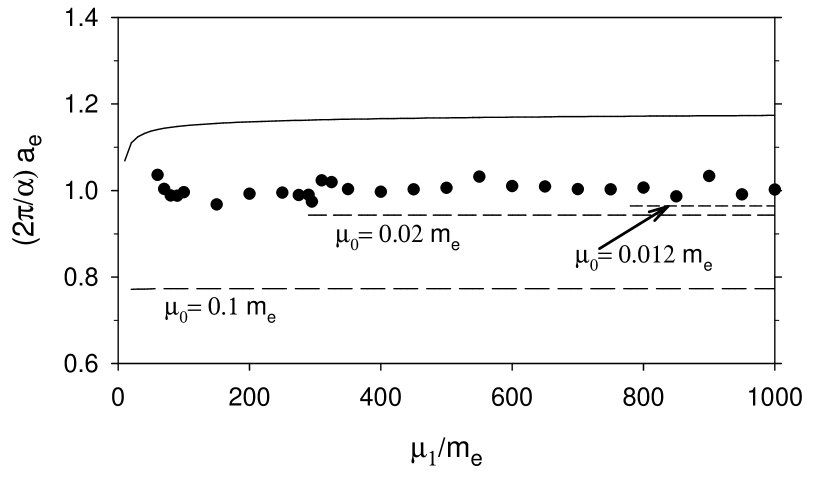
Figure 1: The anomalous moment of the electron in units of the Schwinger term ($\alpha/2\pi$) plotted versus the PV photon mass, $\mu_{1}$. The solid line is the standard-parameterization result for the one-electron/one-photon truncation and the dashed lines are the results for sector-dependent parameterization at three different values of photon mass $\mu_{0}$; both use $m_{1}=\infty$. The results for the sector-dependent parameterization are plotted only for values of $\mu_{1}$ for which the probability of the two-particle sector remains between 0 and 1; for values of $\mu_{0}\leq 0.01m_{e}$, this requires $\mu_{1}>1000m_{e}$, which is beyond the range of the plot. For the case of the standard parameterization, $\mu_{0}$ has its physical value of zero. The filled circles are from a calculation with the standard parameterization that includes the self-energy contribution from the one-electron/two-photon sector. It also includes a second PV photon flavor, with its mass, $\mu_{2}$, set to $\sqrt{2}\mu_{1}$; the PV electron mass $m_{1}$ is equal to $2\cdot 10^{4}\,m_{e}$. The variation is due to errors in numerical quadratures.

For the standard parameterization, $\alpha_{0}=\alpha$, and the normalization is $z_{0}^{2}=1/(1+e^{2}J_{2})$, as given in (25). The anomalous moment is then

$$a_{e} = \frac{\alpha m_{e}^{2}}{\pi(1+e^{2}J_{2})}\int y^{2}(1-y)dydk_{\perp}^{2}$$

$$\times\left(\sum_{k=0}^{1}\frac{(-1)^{k}}{ym_{0}^{2}+(1-y)\mu_{k}^{2}+k_{\perp}^{2}-m_{e}^{2}y(1-y)}\right)^{2}.$$

This is also plotted in Fig. 1. For the plotted range of $\mu_{1}$, the normalization factor is unimportant. The deviation from the Schwinger result is due to the presence of the bare mass in the denominator, and the fact that the anomalous-moment integral is sensitive to constituent masses [18].

Although the sector-dependent approach, which inserts $m_{e}$ for $m_{0}$, would appear to be a simple remedy, the complications already discussed make this choice undesirable. Instead, we can include the physics that does adjust the mass by taking into account the self-energy correction that comes from the one-electron/two-photon truncation [29], which we consider in the next section.

We can also consider the anomalous gravitomagnetic moment, which can be computed from a spin-flip matrix element of the energy-momentum tensor [30]. A result of zero is necessary for any approximation to be deemed faithful to the original symmetries of the field theory [31]. As shown in [30], whenever the initial and final states can be expressed as Fock-state expansions with wave functions that depend on boost-invariant, internal momentum variables, the contributions to the anomalous gravitomagnetic moment are zero, term by term in the Fock expansions. This is precisely the case here, for both the standard and sector-dependent parameterizations, with (2.1) as the Fock expansion to be compared with the expansion used for $|\Psi^{\updownarrow}(P^{+},\vec{P}_{\perp})\rangle$ in Eq. (59) of [30], and the net result for this anomalous moment is therefore zero, as required.

3 Self-Energy Contribution

3.1 Coupled Equations

We extend the equations (6) and (7) for the one-electron/one-photon sector to include coupling to the one-electron/two-photon sector

$$\left[M^{2}-\frac{m_{i}^{2}+q_{\perp}^{2}}{(1-y)}-\frac{\mu_{l}^{2}+q_{\perp}^{2}}{y}\right]C_{ils}^{\mu\pm}(\underline{q})$$

$$= \sqrt{\xi_{l}}\sum_{j}(-1)^{j}z_{j}P^{+}\left[\delta_{s,\pm 1/2}V_{ijs}^{\mu}(\underline{P}-\underline{q},\underline{P})+\delta_{s,\mp 1/2}U_{ij,-s}^{\mu}(\underline{P}-\underline{q},\underline{P})\right]$$

$$+\sum_{ab\nu}(-1)^{a+b}\epsilon^{\nu}\int d\underline{q}^{\prime}\frac{2\sqrt{\xi_{b}}}{\sqrt{1+\delta_{bl}\delta^{\mu\nu}}}\left[V_{ais}^{\nu*}(\underline{P}-\underline{q}^{\prime}-\underline{q},\underline{P}-\underline{q}^{\prime})C_{abls}^{\nu\mu\pm}(\underline{q}^{\prime},\underline{q})\right.$$

$$\rule{144.54pt}{0.0pt}\left.+U_{ais}^{\nu*}(\underline{P}-\underline{q}^{\prime}-\underline{q},\underline{P}-\underline{q}^{\prime})C_{abl,-s}^{\nu\mu\pm}(\underline{q}^{\prime},\underline{q})\right],$$

and add the equation for the new sector

$$\left[M^{2}-\frac{m_{i}^{2}+(\vec{q}_{1\perp}+\vec{q}_{2\perp})^{2}}{(1-y_{1}-y_{2})}-\frac{\mu_{j}^{2}+q_{1\perp}^{2}}{y_{1}}-\frac{\mu_{l}^{2}+q_{2\perp}^{2}}{y_{2}}\right]C_{ijls}^{\mu\nu\pm}(\underline{q}_{1},\underline{q}_{2})$$

$$= \frac{\sqrt{1+\delta_{jl}\delta^{\mu\nu}}}{2}\sum_{a}(-1)^{a}\left\{\sqrt{\xi_{j}}\left[V_{ias}^{\mu}(\underline{P}-\underline{q}_{1}-\underline{q}_{2},\underline{P}-\underline{q}_{2})C_{als}^{\nu\pm}(\underline{q}_{2})\right.\right.$$

$$\rule{144.54pt}{0.0pt}\left.+U_{ia,-s}^{\mu}(\underline{P}-\underline{q}_{1}-\underline{q}_{2},\underline{P}-\underline{q}_{2})C_{al,-s}^{\nu\pm}(\underline{q}_{2})\right]$$

$$\rule{50.58878pt}{0.0pt}+\sqrt{\xi_{l}}\left[V_{ias}^{\nu}(\underline{P}-\underline{q}_{1}-\underline{q}_{2},\underline{P}-\underline{q}_{1})C_{ajs}^{\mu\pm}(\underline{q}_{1})\right.$$

$$\left.\left.\rule{122.85876pt}{0.0pt}+U_{ia,-s}^{\nu}(\underline{P}-\underline{q}_{1}-\underline{q}_{2},\underline{P}-\underline{q}_{1})C_{aj,-s}^{\mu\pm}(\underline{q}_{1})\right]\right\}.$$

This last equation can be solved explicitly for the three-body wave function $C_{ijls}^{\mu\nu\pm}$. Substitution of this into (3.1) and retention of only self-energy contributions for the two-photon intermediate states yields

$$\left[M^{2}-\frac{m_{i}^{2}+q_{\perp}^{2}}{1-y}-\frac{\mu_{l}^{2}+q_{\perp}^{2}}{y}\right]C_{ils}^{\mu\pm}(y,q_{\perp})=S_{ils}^{\mu\pm}+\frac{\alpha}{2\pi}\sum_{i^{\prime}}\frac{I_{ili^{\prime}}(y,q_{\perp})}{1-y}C_{i^{\prime}ls}^{\mu\pm}(y,q_{\perp}),$$ (34)

with $i=0,1$ and $l=0,1,2$. Here the coupling to the bare-electron sector is written as

$$S_{ils}^{\mu\pm}=\sqrt{\xi_{l}}\sum_{j}(-1)^{j}z_{j}P^{+}[\delta_{s,\pm 1/2}V_{ijs}^{\mu}(\underline{P}-\underline{q},\underline{P})+\delta_{s,\mp 1/2}U_{ij,-s}^{\mu}(\underline{P}-\underline{q},\underline{P})],$$ (35)

and the new self-energy contributions are written in terms of the integral

$$I_{ili^{\prime}}(y,q_{\perp}) = (1-y)\frac{2\pi}{\alpha}\sum_{ab\nu}\int\frac{(-1)^{a+b+i^{\prime}}\xi_{b}\epsilon^{\nu}d\underline{q}^{\prime}}{M^{2}-\frac{m_{a}^{2}+(\vec{q}_{\perp}^{\,\prime}+\vec{q}_{\perp})^{2}}{(1-y-y^{\prime})}-\frac{\mu_{b}^{2}+q_{\perp}^{\prime 2}}{y^{\prime}}-\frac{\mu_{l}^{2}+q_{\perp}^{2}}{y}}$$

$$\rule{28.90755pt}{0.0pt}\times\left[V_{ais}^{\nu*}(\underline{P}-\underline{q}^{\prime}-\underline{q},\underline{P}-\underline{q}^{\prime})V_{ai^{\prime}s}^{\nu}(\underline{P}-\underline{q}^{\prime}-\underline{q},\underline{P}-\underline{q})\right.$$

$$\rule{43.36243pt}{0.0pt}\left.+U_{ais}^{\nu*}(\underline{P}-\underline{q}^{\prime}-\underline{q},\underline{P}-\underline{q}^{\prime})U_{ai^{\prime}s}^{\nu}(\underline{P}-\underline{q}^{\prime}-\underline{q},\underline{P}-\underline{q})\right].$$

These, combined with the coupled equation (2.2) for the one-body amplitude, constitute the eigenvalue problem when only the self-energy contributions of the two-photon states are included. A diagrammatic representation is given in Fig. 2.

Figure 2: Diagrammatic representation of the coupled equations (2.2) and (34) of the text. The filled circles and ovals represent wave functions for Fock states; the solid lines represent fermions; and the dashed lines represent photons. The crosses on lines represent the light-cone kinetic energy contributions, which are summed over all particles in the Fock state.

The self-energy integral can be written in simpler form. The change of variables $x=q^{\prime+}/q^{+}=y^{\prime}/(1-y)$ and $\vec{k}_{\perp}=\vec{q}_{\perp}^{\,\prime}+x\vec{q}_{\perp}$ yields

$$I_{ili^{\prime}}(y,q_{\perp})=\sum_{a,b}(-1)^{i^{\prime}+a+b}\xi_{b}\int_{0}^{1}\frac{dx}{x}\frac{d^{2}k_{\perp}}{\pi}\frac{m_{i}m_{i^{\prime}}-2\frac{m_{i}+m_{i^{\prime}}}{1-x}m_{a}+\frac{m_{a}^{2}+k_{\perp}^{2}}{(1-x)^{2}}}{\Lambda_{l}-\frac{m_{a}^{2}+k_{\perp}^{2}}{1-x}-\frac{\mu_{b}^{2}+k_{\perp}^{2}}{x}},$$ (37)

which, on use of $\bar{I}_{0}$, $\bar{I}_{1}$, and $\bar{J}$ defined in Eqs. (11) and (12), can be written as

$$I_{ili^{\prime}}(y,q_{\perp})=16\pi^{2}(-1)^{i^{\prime}}\left[m_{i}m_{i^{\prime}}\bar{I}_{0}(\Lambda_{l})-2(m_{i}+m_{i^{\prime}})\bar{I}_{1}(\Lambda_{l})+\bar{J}(\Lambda_{l})\right],$$ (38)

with

$$\Lambda_{l}\equiv\mu_{l}^{2}+(1-y)M^{2}-\frac{\mu_{l}^{2}+q_{\perp}^{2}}{y}.$$ (39)

For $\bar{J}$ we still have the identity $\bar{J}(\Lambda_{l})=\Lambda_{l}\bar{I}_{0}(\Lambda_{l})$. The integrals can be evaluated analytically, but, for extreme values of the momentum, such as momentum fractions on the order of $(m_{0}/m_{1})^{2}\sim 10^{-10}$, evaluation of the analytic form suffers from round-off error due to the finite precision available in floating-point calculations. The self-energy is then best computed by numerical evaluation of the longitudinal integrals. Notice that $I_{ili^{\prime}}$ includes a flavor changing self-energy, where the index $i^{\prime}$ is different from the index $i$; this is a result of the flavor changing currents used in the interaction Lagrangian (A).

The solution for the coupling constant and the one-electron amplitudes $z_{i}$ is

$$\alpha_{\pm} = \frac{G_{00}+G_{11}\pm\sqrt{(G_{00}-G_{11})^{2}-4G_{10}G_{01}}}{16\pi[G_{00}G_{11}-G_{10}G_{01}]},$$ (40)

$$\frac{z_{1}}{z_{0}} = \frac{[G_{11}-G_{00}]/2\mp\sqrt{(G_{00}-G_{11})^{2}-4G_{10}G_{01}}}{G_{01}},$$ (41)

with

$$G_{il}=\frac{(-1)^{l}}{M^{2}-m_{i}^{2}}[m_{i}m_{l}\tilde{I}_{0}-2(m_{i}+m_{l})\tilde{I}_{1}+\tilde{J}]$$ (42)

and the integrals $\tilde{I}_{n}$ and $\tilde{J}$ defined in (69). Details of the solution are given in B. We again have $\alpha$ as a function of $m_{0}$ and the PV masses, and we seek the value of $m_{0}$ that yields the physical value of $\alpha$. The calculation requires numerical quadrature of the integrals $\tilde{I}_{n}$ and $\tilde{J}$; this can be done with the quadrature schemes discussed in [13] and [29].

3.2 Anomalous Moment

The wave functions $C_{ijs}^{\mu\pm}$ can be used to compute the anomalous moment. Since $\tilde{J}$ does not satisfy any known identity, it cannot be eliminated. Therefore, the calculation must be done at finite $m_{1}$, and the second PV photon flavor must be kept [14]. However, the calculation can still be done [29].

The results are included in Fig. 1. The value of the PV electron mass $m_{1}$ is chosen to be $2\cdot 10^{4}\,m_{e}$, which was found in the case of the one-photon truncation to be sufficiently large [14]. The ratio of PV photon masses $\mu_{2}/\mu_{1}$ is held fixed at $\sqrt{2}$, and $\mu_{1}$ is varied. As for the choice of $m_{1}$, this choice was found sufficient in [14]. The results are consistent with perturbative QED, showing only variations expected from numerical errors of order 1% in calculating the underlying integrals $\tilde{I}_{n}$ and $\tilde{J}$.

That the self-energy contribution brings the result so close to the leading Schwinger contribution is clear from the following. The dominant contribution to the expression (2.4) for the anomalous moment is the $j=0$, $i=i^{\prime}=0$, and $k=k^{\prime}=0$ contribution to the first term; the other terms are suppressed by the large PV masses that appear in the denominators of the wave functions $C_{iks}^{\mu\pm}(\underline{k})$. For the dominant term, the denominator, as determined by (67) and (65), is essentially the square of

$$A_{00}=\frac{m_{0}^{2}+\frac{\alpha}{2\pi}I_{000}+q_{\perp}^{2}}{1-y}+\frac{\mu_{0}^{2}+q_{\perp}^{2}}{y}-m_{e}^{2},$$ (43)

with

$$I_{000}=16\pi^{2}[(m_{0}^{2}+\Lambda_{0})\bar{I}_{0}(\Lambda_{0})-4m_{0}\bar{I}_{1}(\Lambda_{0})]$$ (44)

and

$$\Lambda_{0}=\mu_{0}^{2}+(1-y)m_{e}^{2}-\frac{\mu_{0}^{2}+q_{\perp}^{2}}{y},$$ (45)

from the expressions in (37) and (39). For the physical photon, $\mu_{0}$ is zero, and the two-body wave function is peaked at $q_{\perp}=0$ and $y=0$, so that we can approximate $\Lambda_{0}$ as $m_{e}^{2}$. We then have

$$A_{00}\simeq\frac{m_{0}^{2}+8\pi\alpha[(m_{0}^{2}+m_{e}^{2})\bar{I}_{0}(m_{e}^{2})-4m_{0}\bar{I}_{1}(m_{e}^{2})]+q_{\perp}^{2}}{1-y}+\frac{q_{\perp}^{2}}{y}-m_{e}^{2}$$ (46)

In our formulation, the perturbative one-loop electron self-energy can be read from Eq. (10) for $i=0$, with $z_{1}=0$, $M^{2}=m_{0}^{2}+\delta m^{2}$ on the left, and $M^{2}=m_{0}^{2}$ on the right. This yields

$$\delta m^{2}=m_{0}^{2}-m_{e}^{2}=2e^{2}\left[m_{0}^{2}\bar{I}_{0}(m_{0}^{2})-4m_{0}\bar{I}_{1}(m_{0}^{2})+\bar{J}(m_{0}^{2})\right].$$ (47)

From this mass shift, we have, to leading order in $\alpha=e^{2}/4\pi$, with use of the identity $\bar{J}(m_{0}^{2})=m_{0}^{2}\bar{I}_{0}(m_{0}^{2})$,

$$m_{0}^{2}=m_{e}^{2}-8\pi\alpha[(m_{0}^{2}+m_{e}^{2})\bar{I}_{0}(m_{e}^{2})-4m_{0}\bar{I}_{1}(m_{e}^{2})].$$ (48)

Therefore, the denominator reduces to the square of

$$A_{00}=\frac{m_{e}^{2}+q_{\perp}^{2}}{1-y}+\frac{q_{\perp}^{2}}{y}-m_{e}^{2}+{\cal O}(\alpha^{2}),$$ (49)

which matches the denominator of the integral (30) that yields the Schwinger contribution. Thus, the dominant contribution to the anomalous moment with the self-energy included is essentially the same as the integral that yields the Schwinger result.

4 Summary

In the calculation presented here, we have continued the development of nonperturbative Pauli–Villars regularization and light-front Hamiltonian techniques as a method for the determination of bound-state wave functions in quantum field theories. The new results extend previous work on QED [12, 14] to include some of the effects of one-electron/two-photon Fock states; the previous work was limited to a one-electron/one-photon truncation. To reach agreement with the Schwinger result for the anomalous moment [26] is meant as a test of the method but not as the purpose of the method. Instead, the method is intended for strongly coupled theories, where perturbation theory is not applicable. Applications of the method to a gauge theory are important as precursors to applications to QCD.

We have also shown that use of a sector-dependent parameterization [17, 18, 19] requires great care in the handling of an infrared divergence and an uncanceled ultraviolet divergence. The expression for the anomalous moment is itself safe from these divergences, and one is led to think that regulators can be removed. However, the underlying theory is not safe and quickly enters an unphysical regime, if care is not taken. The bare coupling becomes imaginary, the Fock-state wave functions become ill-defined, and the Fock-sector probabilities fall outside the interval $[0,1]$.

The infrared and ultraviolet divergences are interconnected. The infrared divergence is regulated by the introduction of a nonzero mass for the physical photon, but the result for the anomalous moment of the electron does not agree with experiment unless this mass is quite small. In turn, a small physical photon mass requires a large PV photon mass to keep Fock-sector probabilities within the physical range of zero to one. Unfortunately, a large PV photon mass can lead to great difficulties for a numerical calculation with a higher-order Fock truncation, as was seen in [29].

The standard parameterization does not have an infrared problem and has no particular difficulty with its own uncanceled ultraviolet divergence. The Fock-state wave functions are well defined. The one-electron/one-photon truncation does yield [14] an anomalous moment that is 17% larger than the experimental value; in a sense, it includes too much physics from higher orders in $\alpha$. The discrepancy with experiment, which is unrelated to the uncanceled divergence, is immediately corrected by the self-energy contribution from the one-electron/two-photon sector, which adjusts the constituent electron mass that appears in the anomalous moment integral. The sector-dependent approach, in effect, attempts to incorporate this correction by forcing the constituent mass to be equal to the physical mass, which causes the infrared divergence. Thus, the standard approach is to be preferred, at least for gauge theories.

Appendix A Feynman-gauge QED

The PV-regulated Feynman-gauge QED Lagrangian is

$${\cal L} = \sum_{i=0}^{2}(-1)^{i}\left[-\frac{1}{4}F_{i}^{\mu\nu}F_{i,\mu\nu}+\frac{1}{2}\mu_{i}^{2}A_{i}^{\mu}A_{i\mu}-\frac{1}{2}\left(\partial^{\mu}A_{i\mu}\right)^{2}\right]$$

$$+\sum_{i=0}^{1}(-1)^{i}\bar{\psi_{i}}(i\gamma^{\mu}\partial_{\mu}-m_{i})\psi_{i}-e_{0}\bar{\psi}\gamma^{\mu}\psi A_{\mu},$$

where

$$A_{\mu}=\sum_{i=0}^{2}\sqrt{\xi_{i}}A_{i\mu},\;\;\psi=\sum_{i=0}^{1}\psi_{i},\;\;F_{i\mu\nu}=\partial_{\mu}A_{i\nu}-\partial_{\nu}A_{i\mu}.$$ (51)

The subscript $i=0$ denotes a physical field and $i=1$ or 2 a PV field. Fields with odd index $i$ are chosen to be negatively normed. The constants $\xi_{i}$ satisfy the following constraints [14]:

$$\xi_{0}=1,$$ (52)

$$\sum_{i=0}^{2}(-1)^{i}\xi_{i}=0,$$ (53)

$$\sum_{i=0}^{2}(-1)^{i}\xi_{i}\frac{\mu_{i}^{2}/m_{1}^{2}}{1-\mu_{i}^{2}/m_{1}^{2}}\ln(\mu_{i}^{2}/m_{1}^{2})=0.$$ (54)

The second constraint guarantees the necessary cancellations for ultraviolet regularization; it also implies that $A^{\mu}$ in (51) is a zero-norm field. The third guarantees the correct chiral limit at one loop; for truncations that include higher loops, there are order-$\alpha$ corrections to the constraint. Implementation of the gauge condition $\partial^{\mu}A_{i\mu}=0$ is discussed in [14].

When the PV electron mass is sufficiently large, the third constraint (54) can be approximated by

$$\sum_{l}(-1)^{l}\xi_{l}\mu_{l}^{2}\ln(\mu_{l}/m_{1})=0.$$ (55)

The solution to the set of constraints, (52), (53), and (55), assuming $\mu_{0}=0$, is then

$$\xi_{1}=1+\xi_{2}\;\;\mbox{and}\;\;\xi_{2}=\frac{\mu_{1}^{2}\ln(\mu_{1}/m_{1})}{\mu_{2}^{2}\ln(\mu_{2}/m_{1})-\mu_{1}^{2}\ln(\mu_{1}/m_{1})}.$$ (56)

Without loss of generality, we require $\mu_{2}>\mu_{1}$, so that $\xi_{2}$ is positive.

The dynamical fields are

$$\psi_{i+} = \frac{1}{\sqrt{16\pi^{3}}}\sum_{s}\int d\underline{k}\chi_{s}\left[b_{is}(\underline{k})e^{-i\underline{k}\cdot\underline{x}}+d_{i,-s}^{\dagger}(\underline{k})e^{i\underline{k}\cdot\underline{x}}\right]\,,$$ (57)

$$A_{i\mu} = \frac{1}{\sqrt{16\pi^{3}}}\int\frac{d\underline{k}}{\sqrt{k^{+}}}\left[a_{i\mu}(\underline{k})e^{-i\underline{k}\cdot\underline{x}}+a_{i\mu}^{\dagger}(\underline{k})e^{i\underline{k}\cdot\underline{x}}\right]\,,$$ (58)

with [32] $\chi_{s}$ an eigenspinor of $\Lambda_{+}\equiv\gamma^{0}\gamma^{+}/2$. The creation and annihilation operators satisfy (anti)commutation relations

$$\{b_{is}(\underline{k}),b_{i^{\prime}s^{\prime}}^{\dagger}(\underline{k}^{\prime}\} = (-1)^{i}\delta_{ii^{\prime}}\delta_{ss^{\prime}}\delta(\underline{k}-\underline{k}^{\prime}),$$ (59)

$$\{d_{is}(\underline{k}),d_{i^{\prime}s^{\prime}}^{\dagger}(\underline{k}^{\prime}\} = (-1)^{i}\delta_{ii^{\prime}}\delta_{ss^{\prime}}\delta(\underline{k}-\underline{k}^{\prime}),$$ (60)

$${[}a_{i\mu}(\underline{k}),a_{i^{\prime}\nu}^{\dagger}(\underline{k}^{\prime}] = (-1)^{i}\delta_{ii^{\prime}}\epsilon^{\mu}\delta_{\mu\nu}\delta(\underline{k}-\underline{k}^{\prime}).$$ (61)

Here $\epsilon^{\mu}=(-1,1,1,1)$ is the metric signature for the photon field components in Gupta–Bleuler quantization [33, 34].

Without antifermion terms, the Hamiltonian is

$${\cal P}^{-}=\sum_{i,s}\int d\underline{p}\frac{m_{i}^{2}+p_{\perp}^{2}}{p^{+}}(-1)^{i}b_{i,s}^{\dagger}(\underline{p})b_{i,s}(\underline{p})$$

$$+\sum_{l,\mu}\int d\underline{k}\frac{\mu_{l}^{2}+k_{\perp}^{2}}{k^{+}}(-1)^{l}\epsilon^{\mu}a_{l\mu}^{\dagger}(\underline{k})a_{l\mu}(\underline{k})$$

$$+\sum_{i,j,l,s,\mu}\int d\underline{p}d\underline{q}\left\{b_{i,s}^{\dagger}(\underline{p})\left[b_{j,s}(\underline{q})V^{\mu}_{ij,2s}(\underline{p},\underline{q})\right.\right.$$

$$\left.\left.\rule{36.135pt}{0.0pt}+b_{j,-s}(\underline{q})U^{\mu}_{ij,-2s}(\underline{p},\underline{q})\right]\sqrt{\xi_{l}}a_{l\mu}^{\dagger}(\underline{q}-\underline{p})+H.c.\right\}.$$

The vertex functions are [12]

$$V^{0}_{ij\pm}(\underline{p},\underline{q}) = \frac{e_{0}}{\sqrt{16\pi^{3}}}\frac{\vec{p}_{\perp}\cdot\vec{q}_{\perp}\pm i\vec{p}_{\perp}\times\vec{q}_{\perp}+m_{i}m_{j}+p^{+}q^{+}}{p^{+}q^{+}\sqrt{q^{+}-p^{+}}},$$ (63)

$$V^{3}_{ij\pm}(\underline{p},\underline{q}) = \frac{-e_{0}}{\sqrt{16\pi^{3}}}\frac{\vec{p}_{\perp}\cdot\vec{q}_{\perp}\pm i\vec{p}_{\perp}\times\vec{q}_{\perp}+m_{i}m_{j}-p^{+}q^{+}}{p^{+}q^{+}\sqrt{q^{+}-p^{+}}},$$

$$V^{1}_{ij\pm}(\underline{p},\underline{q}) = \frac{e_{0}}{\sqrt{16\pi^{3}}}\frac{p^{+}(q^{1}\pm iq^{2})+q^{+}(p^{1}\mp ip^{2})}{p^{+}q^{+}\sqrt{q^{+}-p^{+}}},$$

$$V^{2}_{ij\pm}(\underline{p},\underline{q}) = \frac{e_{0}}{\sqrt{16\pi^{3}}}\frac{p^{+}(q^{2}\mp iq^{1})+q^{+}(p^{2}\pm ip^{1})}{p^{+}q^{+}\sqrt{q^{+}-p^{+}}},$$

$$U^{0}_{ij\pm}(\underline{p},\underline{q}) = \frac{\mp e_{0}}{\sqrt{16\pi^{3}}}\frac{m_{j}(p^{1}\pm ip^{2})-m_{i}(q^{1}\pm iq^{2})}{p^{+}q^{+}\sqrt{q^{+}-p^{+}}},$$

$$U^{3}_{ij\pm}(\underline{p},\underline{q}) = \frac{\pm e_{0}}{\sqrt{16\pi^{3}}}\frac{m_{j}(p^{1}\pm ip^{2})-m_{i}(q^{1}\pm iq^{2})}{p^{+}q^{+}\sqrt{q^{+}-p^{+}}},$$

$$U^{1}_{ij\pm}(\underline{p},\underline{q}) = \frac{\pm e_{0}}{\sqrt{16\pi^{3}}}\frac{m_{i}q^{+}-m_{j}p^{+}}{p^{+}q^{+}\sqrt{q^{+}-p^{+}}},$$

$$U^{2}_{ij\pm}(\underline{p},\underline{q}) = \frac{ie_{0}}{\sqrt{16\pi^{3}}}\frac{m_{i}q^{+}-m_{j}p^{+}}{p^{+}q^{+}\sqrt{q^{+}-p^{+}}}.$$

For the standard approach, $m_{0}$ is the same for all sectors and $e_{0}$ is just $e$, there being no fermion-antifermion loops included in the calculation. For the sector-dependent approach, $m_{0}$ and $e_{0}$ depend on the Fock sector where the Hamiltonian is applied. The sector-dependent constants could more generally be functions of momentum [17, 18], but here we follow [19] and use them as constants.

Appendix B Solution for the Self-Energy Contribution

The two-body integral equations (34) can be expressed compactly as

$$A_{0j}C_{0js}^{\mu\pm}-B_{j}C_{1js}^{\mu\pm} = -S_{0js}^{\mu\pm}$$ (64)

$$B_{j}C_{0js}^{\mu\pm}+A_{1j}C_{1js}^{\mu\pm} = -S_{1js}^{\mu\pm}.$$

where $A_{ij}$ and $B_{j}$ are defined by

$$A_{ij}=\frac{m_{i}^{2}+q_{\perp}^{2}}{1-y}+\frac{\mu_{j}^{2}+q_{\perp}^{2}}{y}+\frac{\alpha}{2\pi}\frac{I_{iji}}{1-y}-M^{2}$$ (65)

and

$$B_{j}=\frac{\alpha}{2\pi}\frac{I_{1j0}}{1-y}=-\frac{\alpha}{2\pi}\frac{I_{0j1}}{1-y}.$$ (66)

We solve this 2$\times$2 system for the two-body wave functions

$$C_{ijs}^{\mu\pm}=-\frac{A_{1-i,j}S_{ijs}^{\mu\pm}+(-1)^{i}B_{j}S_{1-i,js}^{\mu\pm}}{A_{0j}A_{1j}+B_{j}^{2}}.$$ (67)

Without the self-energy contributions, we have $B_{j}=0$, and the wave functions reduce to the forms given in (8) and (9), with their line of poles whenever $m_{0}<m_{e}$, as discussed in Sec. 2. Here, however, the self-energy contributions make the denominators more complicated. For values of $m_{0}$ that are smaller than $m_{e}$ by an amount of order $\alpha$, there need not be a line of poles. In fact, we find that, for the solution with self-energy contributions, there is no pole in this two-body Fock sector.

Substitution of (67) into (2.2), and use of the expressions (63) for the vertex functions, yields

$$[M^{2}-m_{i}^{2}]z_{i}=2e^{2}\sum_{j}(-1)^{j}z_{j}[m_{i}m_{j}\tilde{I}_{0}-2(m_{i}+m_{j})\tilde{I}_{1}+\tilde{J}],$$ (68)

where

$$\tilde{I}_{0} = \int\frac{dydq_{\perp}^{2}}{16\pi^{2}}\sum_{j}(-1)^{j}\xi_{j}\frac{A_{0j}-A_{1j}-2B_{j}}{y[A_{0j}A_{1j}+B_{j}^{2}]},$$ (69)

$$\tilde{I}_{1} = \int\frac{dydq_{\perp}^{2}}{16\pi^{2}}\sum_{j}(-1)^{j}\xi_{j}\frac{m_{1}A_{0j}-m_{0}A_{1j}-(m_{0}+m_{1})B_{j}}{y(1-y)[A_{0j}A_{1j}+B_{j}^{2}]},$$

$$\tilde{J} = \int\frac{dydq_{\perp}^{2}}{16\pi^{2}}\sum_{j}(-1)^{j}\xi_{j}$$

$$\times\frac{(m_{1}^{2}+q_{\perp}^{2})A_{0j}-(m_{0}^{2}+q_{\perp}^{2})A_{1j}-2(m_{0}m_{1}+q_{\perp}^{2})B_{j}}{y(1-y)^{2}[A_{0j}A_{1j}+B_{j}^{2}]}.$$

When the self-energy contributions are neglected, these return to the previous expressions Eq. (11) and (12) for $\bar{I}_{0}$, $\bar{I}_{1}$, and $\bar{J}$ in the one-photon truncation. What is more, the eigenvalue equation for $z_{i}$ has nearly the same form as the eigenvalue equation (10) in the one-photon case. The only difference in finding the analytic solution is that $\tilde{I}_{0}$ and $\tilde{J}$ are not connected by any known identity.

References

• [1] For reviews, see M. Creutz, L. Jacobs and C. Rebbi, Phys. Rep. 93 (1983), 201; J.B. Kogut, Rev. Mod. Phys. 55 (1983), 775; I. Montvay, ibid59 (1987), 263; A.S. Kronfeld and P.B. Mackenzie, Ann. Rev. Nucl. Part. Sci. 43 (1993), 793; J.W. Negele, Nucl. Phys. A553 (1993), 47c; K.G. Wilson, Nucl. Phys. B (Proc. Suppl.) 140 (2005), 3; J.M. Zanotti, PoS LAT2008 (2008) 007.
• [2] C.D. Roberts and A.G. Williams, Prog. Part. Nucl. Phys. 33 (1994), 477; P. Maris and C.D. Roberts, Int. J. Mod. Phys. E12 (2003), 297; P.C. Tandy, Nucl. Phys. B (Proc. Suppl.) 141 (2005), 9.
• [3] For reviews, see M. Burkardt, Adv. Nucl. Phys. 23 (2002), 1; S.J. Brodsky, H.-C. Pauli, and S.S. Pinsky, Phys. Rep. 301 (1998), 299.
• [4] M. Burkardt and S. Dalley, Prog. Part. Nucl. Phys.  48 (2002), 317, and references therein; S. Dalley and B. van de Sande, Phys. Rev. D 67 (2003), 114507; D. Chakrabarti, A.K. De, and A. Harindranath, Phys. Rev. D 67 (2003), 076004; M. Harada and S. Pinsky, Phys. Lett. B 567 (2003), 277; S. Dalley and B. van de Sande, Phys. Rev. Lett.  95 (2005), 162001; J. Bratt, S. Dalley, B. van de Sande, and E. M. Watson, Phys. Rev.  D 70 (2004), 114502.
• [5] S.J. Brodsky, R. Roskies, and R. Suaya, Phys. Rev. D 8 (1973), 4574.
• [6] W. Pauli and F. Villars, Rev. Mod. Phys. 21 (1949), 434.
• [7] S.J. Brodsky, J.R. Hiller, and G. McCartor, Phys. Rev. D 58 (1998), 025005.
• [8] S.J. Brodsky, J.R. Hiller, and G. McCartor, Phys. Rev. D 60 (1999), 054506.
• [9] S.J. Brodsky, J.R. Hiller, and G. McCartor, Phys. Rev. D 64 (2001), 114023.
• [10] S.J. Brodsky, J.R. Hiller, and G. McCartor, Ann. Phys. 296 (2002), 406.
• [11] S.J. Brodsky, J.R. Hiller, and G. McCartor, Ann. Phys. 305 (2003), 266.
• [12] S.J. Brodsky, V.A. Franke, J.R. Hiller, G. McCartor, S.A. Paston, and E.V. Prokhvatilov, Nucl. Phys. B 703 (2004), 333.
• [13] S.J. Brodsky, J.R. Hiller, and G. McCartor, Ann. Phys. 321 (2006), 1240.
• [14] S.S. Chabysheva and J.R. Hiller, Phys. Rev. D 79 (2009), 114017.
• [15] B. Grinstein, D. O’Connell, and M.B. Wise, Phys. Rev. D 77 (2008), 025012; C.D. Carone and R.F. Lebed, JHEP 0901 (2009), 43.
• [16] S.A. Paston and V.A. Franke, Theor. Math. Phys.  112 (1997), 1117 [Teor. Mat. Fiz.  112 (1997), 399], [arXiv:hep-th/9901110]; S.A. Paston, V.A. Franke, and E.V. Prokhvatilov, Theor. Math. Phys.  120 (1999), 1164 [Teor. Mat. Fiz.  120 (1999), 417], [arXiv:hep-th/0002062].
• [17] R.J. Perry, A. Harindranath, and K.G. Wilson, Phys. Rev. Lett. 65 (1990), 2959; R.J. Perry and A. Harindranath, Phys. Rev. D 43 (1991), 4051.
• [18] J.R. Hiller and S.J. Brodsky, Phys. Rev. D 59 (1998), 016006.
• [19] V. A. Karmanov, J. F. Mathiot, and A. V. Smirnov, Phys. Rev. D 77 (2008), 085028.
• [20] T. Kinoshita and M. Nio, Phys. Rev.  D 73 (2006), 013003.
• [21] H.-C. Pauli and S.J. Brodsky, Phys. Rev. D 32 (1985), 1993; 32 (1985), 2001.
• [22] V. A. Karmanov and P. Maris, Few Body Syst.  46 (2009), 95.
• [23] G. Baym, Phys. Rev. 117 (1960), 886.
• [24] S.S. Chabysheva and J.R. Hiller, Phys. Rev. D 79 (2009), 096012.
• [25] P.A.M. Dirac, Rev. Mod. Phys. 21 (1949), 392.
• [26] J. Schwinger, Phys. Rev. 73 (1948), 416; 76 (1949), 790.
• [27] D. Mustaki, S. Pinsky, J. Shigemitsu, and K. Wilson, Phys. Rev. D 43 (1991), 3411.
• [28] S.J. Brodsky and S.D. Drell, Phys. Rev. D 22 (1980), 2236.
• [29] S.S. Chabysheva, A nonperturbative calculation of the electron’s anomalous magnetic moment, Ph.D. thesis, Southern Methodist University, ProQuest Dissertations & Theses 3369009 (2009).
• [30] S.J. Brodsky, D.S. Hwang, B.-Q. Ma, and I. Schmidt, Nucl. Phys.  B 593 (2001), 311.
• [31] L. Okun and I.Yu. Kobsarev, JETP 16 (1963), 1343 [ZhETF 43 (1962), 1904]; L. Okun, in the proceedings of the 4th International Conference on Elementary Particles, Heidelberg, Germany (1967), edited by H. Filthuth (North-Holland, Amsterdam, 1968); I.Yu. Kobsarev and V.I. Zakharov, Ann. Phys. (NY) 60 (1970), 448.
• [32] G.P. Lepage and S.J. Brodsky, Phys. Rev. D 22 (1980), 2157.
• [33] S.N. Gupta, Proc. Phys. Soc. (London) A63 (1950), 681; K. Bleuler, Helv. Phys. Acta 23 (1950), 567.
• [34] N.N. Bogoliubov and D.V. Shirkov, Introduction to the Theory of Quantized Fields, (Interscience, New York, 1959); S. Schweber, An Introduction to Relativistic Quantum Field Theory, (Harper & Row, New York, 1961); C. Itzykson and J.-B. Zuber, Quantum Field Theory, (McGraw–Hill, New York, 1980).