Large $N_{c}$ Confinement, Universal Shocks and Random Matrices

Abstract

We study the fluid-like dynamics of eigenvalues of the Wilson operator in the context of the order-disorder (Durhuus-Olesen) transition in large $N_{c}$ Yang-Mills theory. We link the universal behavior at the closure of the gap found by Narayanan and Neuberger to the phenomenon of spectral shock waves in the complex Burgers equation, where the role of viscosity is played by $1/N_{c}$. Next, we explain the relation between the universal behavior of eigenvalues and certain class of random matrix models. Finally, we conlude the discussion of universality by recalling exact analogies between Yang-Mills theories at large $N_{c}$ and the so-called diffraction catastrophes.

PACS numbers come here

1 Introduction

Many efforts continue to be devoted to the study of QCD in the limit of a large number of colors, after the initial suggestion by t’Hooft [1]. This, in part, is due to the general belief that the large $N_{c}$ limit captures the essence of confinement, one of the most elusive of QCD properties. At the same time the theory simplifies considerably in the large $N_{c}$ limit: fluctuations die out and the measure of integration over field configurations in the partition function becomes localized at one particular configuration, making the large $N_{c}$ limit akin to a classical approximation [2].

Many results have been obtained in the simple case of 2 dimensions. Then Yang-Mills theory translates into a large $N_{c}$ matrix model, where the size of the unitary matrix is identified with the number of colors. More specifically, the basic observable that one considers is the Wilson loop along a (simple) curve ${\cal C}$

$$W[A]=P{\rm e}^{i\oint_{\cal C}A_{\mu}dx_{\mu}},$$ (1)

where $A_{\mu}=A_{\mu}^{a}T^{a}$, with $T^{a}$ the generators of SU($N_{c}$) in some representation. In the fundamental representation, $W[A]$ is an $N_{c}\times N_{c}$ unitary matrix with unit determinant. Its eigenvalues are of the form $\lambda=\exp(i\theta)$ and can be associated with points on the unit circle. After averaging over the gauge field configurations, with the usual Yang-Mills measure, one finds that $W=<W[A]>$ depends in fact only on the area ${\cal A}$ enclosed by ${\cal C}$, to within a normalization [3]. It is convenient to measure the area in units of the t’Hooft coupling $g^{2}N_{c}$, i.e., we set $\tau\sim g^{2}N_{c}{\cal A}$. In the limit $N_{c}\to\infty$, the eigenvalues are distributed on the unit circle according to an average density $\rho(\theta,{\tau})$.

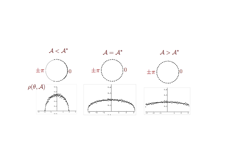
Figure 1: The evolution of the spectral density as a function of the area ${\cal A}$ of the average Wilson loop (d=2). The plots of $\rho(\theta,{\cal A})$ at the bottom are taken from the simulations of Ref. [6].

The typical behavior of the distribution of eigenvalues as a function of the area is displayed in Fig. 1. One observes that for small loops (which probe short distance, perturbative phyics), the spectrum does not cover the whole unit circle, but exhibits a gap; in contrast, for very large loops (which probe long distance, nonperturbative physics) the spectrum covers uniformly the unit circle (gapless phase). This behaviour of the spectrum agrees with the order (gapped)-disorder (gapless) transition, proposed by Durhuus and Olesen [3] and based on the explicit solution of the corresponding Makeenko-Migdal equations [4] in 2 dimensions. Surprisingly, a similar critical behavior has been observed also in $d=3$ dimensions and conjectured to hold in $d=4$ large $N_{c}$ Yang-Mills theory [5], suggesting a universal behavior (see the lectures by Neuberger and Narayanan in these volume, to which we also refer for a discussion of the subtleties of the regularization of the Wilson loops).

This universality conjectured by Narayanan and Neuberger is comforted by simple schematic matrix models, in particular that proposed by Janik and Wieczorek [6], hereafter JW model. The model stems from the general construction of multiplicative free evolution [7], where increments are mutually free in the sense of Voiculescu [8, 9]. The unitary realization in the JW model corresponds to matrix value unitary random walk, where the evolution operator is the ordered string of consecutive multiplications of infinitely large unitary matrices

$$W=\left<\prod_{k}^{K}U_{k}\right>,$$ (2)

where $U_{k}=\exp i\left(\sqrt{t/K}H_{k}\right)$, with $H_{k}$ a hermitian random matrix, drawn from a Gaussian probability distribution $P(H)$ of the form

$$P(H)\sim{\rm e}^{-N{\rm Tr}V(H)}\quad\langle\frac{1}{N}{\rm Tr}H\rangle=0\quad\langle\frac{1}{N}{\rm Tr}H^{2}\rangle=m_{2}.$$ (3)

The model is a random matrix generalization of the multiplicative random walk performed in $K$ steps during “time” $t$. In the continuum limit $K\rightarrow\infty$, the model is exactly solvable. The solution for the spectral density coincides exactly with that of the two-dimensional QCD, provided one identifies $t$ with the area of the Wilson loop, modulo a normalization  [10]. This model offers a neat picture for the multiplicative evolution: at $t=0$, the spectrum of $W$ is localized at $\lambda=1$. As $t$ increases, the spectrum starts to spread symmetrically along the unit circle towards the point $\lambda=-1$, reaching this point and closing the gap at finite time. Further evolution corresponds to further spreading of eigenvalues around the circle, resulting finally in a uniform distribution (see Fig. 1).

Neuberger and Narayanan [5] have observed, that large $N_{c}$ Yang-Mills lattice simulations in $d=2$ and $d=3$ demonstrate the same critical scaling at the closure of the gap as in the JW model and have conjectured that this model establishes a universality class for $d=4$ large $N_{c}$ Yang-Mills theory as well. In their simulations, Narayanan and Neuberger [5] did not calculate the spectral density directly, but rather the average characteristic polynomial

$$Q_{N_{c}}(z,t)\equiv\langle{\rm det}(z-W(t))\rangle.$$ (4)

As we shall see later, this contains the same information as the spectral density when $N_{c}\to\infty$. Narayanan and Neuberger performed simulations at finite $N_{c}$ and obtained evidence that the crossover region between the gapped and gapless regimes is becoming infinitely thin as $N_{c}\rightarrow\infty$.

2 Spectral density and resolvent

The object at the heart of our discussion will be the average density of eigenvalues $\rho(\theta,\tau)$, defined so that the number of eigenvalues of the Wilson operator in the interval $[\theta,\theta+d\theta]$, after averaging over the gauge field configurations loops of a given area ${\cal A}\sim\tau$, is $\rho(\theta,\tau)d\theta$.

2.1 The spectral density and its moments

The spectral density $\rho(\theta,\tau)$ is not available in analytic form, but its moments

$$w_{n}(\tau)\equiv<{\rm tr}\left[W[A]\right]^{n}>_{\tau}=\int_{-\pi}^{+\pi}d\theta\,{\rm e}^{in\theta}\rho(\theta,\tau)$$ (5)

are. An explicit, compact form for these moments is given in Ref. [14] in terms of an integral representation

$$w_{n}(\tau) = \frac{1}{n}\oint\frac{dz}{2\pi i}(1+1/z)^{n}\exp(-n\tau(z+1/2))$$ (6)

$$= \frac{1}{n}L_{(n-1)}^{1}(n\tau)\exp(-n\tau/2)$$

where the representation of Laguerre polynomials, used in the second line, allows connection to results known already 25 years ago [3, 11].

The Durhuus-Olesen transition can be seen by studying the asymptotic behavior of these Laguerre polynomials, using a saddle point analysis of their integral representation  [12, 13]. The result is surprising: for a loop area below the critical value $\tau_{c}=4$, the moments oscillate and decay like $n^{-3/2}$, while for $\tau>\tau_{c}$ the moments decay exponentially with $n$, modulo similar power behavior. Both regimes are separated by a double scaling limit.

Let us quote here the values of the first couple of moments. The normalization of the spectral density is given by

$$w_{0}=\int_{-\pi}^{\pi}d\theta\rho(\theta)=1.$$ (7)

The first moment expresses the area law obeyed by the average of the Wilson operator

$$w_{1} = {\rm e}^{-\tau/2}.$$ (8)

More generally, since $\rho$ is real, $w_{n}^{*}=w_{-n}$, and since the moments, as given by the formula above are real, we have ($n>0$) $w_{-n}=w_{n}$. Thus we can express $\rho$ as follows

$$\rho(\theta) = \frac{1}{2\pi}\sum_{m=-\infty}^{+\infty}w_{m}{\rm e}^{-im\theta}$$ (9)

$$= \frac{1}{2\pi}\left(1+\sum_{n=1}^{+\infty}2w_{n}\cos(n\theta)\right).$$

Note that, for $\tau=0$, $w_{n}=1$ for all $n$, and

$$\rho(\theta,\tau=0) = \frac{1}{2\pi}\sum_{m=-\infty}^{+\infty}{\rm e}^{-im\theta}$$ (10)

$$= \sum_{n=-\infty}^{+\infty}\delta(\theta+2n\pi)$$

$$= \delta(\theta)$$

where we used Poisson summation formula, and in the last line the restriction $-\pi<\theta\leq\pi$.

2.2 The resolvent

To the spectral density one may associate a resolvent, defined as

$$G(z)=\int_{-\pi}^{+\pi}d\theta\,\frac{\rho(\theta)}{z-{\rm e}^{i\theta}}.$$ (11)

For $|z|>1$ we can expand the integrand in a power series of ${\rm e}^{i\theta}/z$ and get

$$zG(z)-1=\sum_{n=1}^{\infty}\frac{w_{n}}{z^{n}}\equiv f(z),$$ (12)

where the function $f$ is the same as that introduced in Ref. [6]. By setting $z={\rm e}^{i\alpha}$, we can also write

$$f(z={\rm e}^{i\alpha})=\sum_{n=1}^{\infty}{w_{n}}{\rm e}^{-in\alpha}$$ (13)

with ${\rm Im}\,\alpha<0$ to guarantee the convergence of the sum.

Now we introduce a new function that will play a central role in our discussion. We set [14]:

$$F(z={\rm e}^{i\alpha}) \equiv i\left(f(z)+\frac{1}{2}\right)=i\left(zG(z)-\frac{1}{2}\right)$$ (14)

$$= i\left(\frac{1}{2}+\sum_{n=1}^{+\infty}w_{n}{\rm e}^{-in\alpha}\right),$$

where in the last line we assume ${\rm Im}\,\alpha<0$. The imaginary part of $F$ yields the spectral density ($\theta$ real)

$$\rho(\theta)=\frac{1}{\pi}{\rm Im}F(z={\rm e}^{i\theta}).$$ (15)

We can also write ($\alpha$ and $\theta$ real)

$$F(z={\rm e}^{i\alpha})=i\int_{-\pi}^{+\pi}d\theta\,\rho(\theta)\left\{\frac{{\rm e}^{i\alpha}}{{\rm e}^{i\alpha}-{\rm e}^{i\theta}}-\frac{1}{2}\right\},$$ (16)

so that

$$F(z={\rm e}^{i\alpha})=\frac{1}{2}\int_{-\pi}^{+\pi}d\theta\,\rho(\theta)\cot\left(\frac{\alpha-\theta}{2}\right).$$ (17)

At this point, we shall make an abuse of notation and write $F(\alpha)$ for $F(z={\rm e}^{i\alpha})$, and furthermore we shall allow $\alpha$ to be complex. One can then write, for real $\alpha$

$$\frac{1}{\pi}F(\alpha)=H\rho(\alpha)+i\rho(\alpha),$$ (18)

where $H\rho(\alpha)$ is the Hilbert transform

$$H\rho(\alpha)=\frac{1}{2\pi}P.V.\int_{-\pi}^{+\pi}d\theta\,\rho(\theta)\cot\left(\frac{\alpha-\theta}{2}\right).$$ (19)

Note that there is a choice of sign for the imaginary part, related on where we decide to view $F$ as analytic (lower or upper plane), that is, on how we take the limit from complex $\alpha$ to real $\alpha$. The present choice corresponds to choosing $F$ to be analytic in the lower half-plane.

The following properties of the Hilbert transform will be useful

$$H{\rm e}^{i\alpha}=\frac{1}{2\pi}P.V.\int_{-\pi}^{+\pi}d\theta\,{\rm e}^{i\theta}\cot\left(\frac{\alpha-\theta}{2}\right)=-i{\rm e}^{i\alpha}.$$ (20)

It follows that

$$H\cos\alpha=\sin\alpha\quad H\sin\alpha=-\cos\alpha$$ (21)

We have also

$$H(H(f)) = -f$$

$$H(fg) = fH(g)+gH(f)+H[H(f)H(g)],$$ (22)

from which it follows in particular that

$$H[H(\rho)\rho]=\frac{1}{2}\left((H(\rho))^{2}-\rho^{2}\right).$$ (23)

3 Complex Burgers equation and its solution with characteristics

The usefulness of the function $F$ that we have introduced comes from the fact that it satisfies a simple equation, the complex Burgers equation[14, 3, 11]:

$$\partial_{\tau}F+F\partial_{\theta}F=0.$$ (24)

This equation is analogous to the real Burgers equation of fluid dynamics [15] (with $\tau$ playing the role of time, $\theta$ that of a coordinate, and $F_{0}$ of a velocity field). The complex Burgers equation is omnipresent in Free Random Variables calculus [8]. It also appears frequently as one dimensional models for quasi-geostrophic equations, describing e.g. the dynamics of the mixture of cold and hot air and the fronts between them [16]. Here, we shall take advantage of the abundant mathematical studies of the complex Burgers equation to analyze the flow of eigenvalues of Wilson loop operators. We shall in particular use the crucial fact that the complex Burgers equation may allow for the formation of shocks.

A simple derivation of the complex Burgers equation will be given in Sect. 5 below. In this section we shall analyze general properties of its solutions, using the method of complex characteristics.

3.1 Characteristics

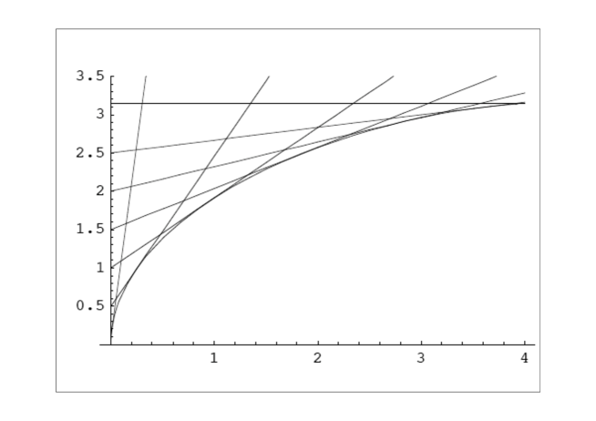
Figure 2: Characteristic lines for $\tau\leq 4$, $\alpha=\xi+\frac{\tau}{2}\cot\frac{\xi}{2}$, with $\alpha=\theta$ real on the vertical axis, and $\tau$ on the horizontal axis. The various straight lines are given by the characteristic equation (33) in which $\xi=x$ is treated as a parameter. The horizontal characteristic corresponds to $x=\pi$, the first one, almost vertical, to $x=0.1$.

The Burgers equation

$$\partial_{\tau}F+F\partial_{\alpha}F=0.$$ (25)

admits the following solution in terms of characteristics

$$F(\tau,\alpha)=F_{0}(\xi(\tau,\alpha)),\qquad F_{0}(\alpha)=F(\tau=0,\alpha),\qquad\alpha=\xi+\tau F_{0}(\xi).$$ (26)

The initial condition $F_{0}$ corresponding to a spectral density peaked at $\theta=0$,

$$\rho_{0}(\theta)=\delta(\theta),$$ (27)

is

$$F_{0}(\alpha)=\frac{1}{2}\cot\frac{\alpha}{2}.$$ (28)

The characteristics are therefore given by

$$\alpha=\xi+\frac{\tau}{2}\cot\frac{\xi}{2},$$ (29)

with $\alpha$ complex. Once $\xi(\alpha,\tau)$ is known, $F(\alpha,\tau)$ can be obtained as $F(\alpha,\tau)=(\alpha-\xi)/\tau$. In particular, for real $\alpha$, we have ${\rm Im}F=-(1/\tau){\rm Im}\xi$, so that $\rho=-y/(\tau\pi)$, with $y={\rm Im}\xi$. Alternatively, one may look for $F$ as the solution of the implicit equation

$$F=\frac{1}{2}\cot\left(\xi+\tau F\right).$$ (30)

We shall set $\xi=x+iy$, and $\alpha=\theta+i\eta$. Then, by taking the real and imaginary parts of the characteristic equation, we get

$$\theta = x+\tau{\rm e}^{y}\,\frac{\sin x}{1-2{\rm e}^{y}\cos x+{\rm e}^{2y}}=x+\frac{\tau}{2}\,\frac{\sin x}{\cosh y-\cos x}$$

$$\eta = y+\frac{\tau}{2}\frac{1-{\rm e}^{2y}}{1-2{\rm e}^{y}\cos x+{\rm e}^{2y}}=y-\frac{\tau}{2}\,\frac{\sinh y}{\cosh y-\cos x}.$$ (31)

The characteristics form a family of straight lines in the $(\theta,\eta)$ plane, $\theta(\tau)$, $\eta(\tau)$, that depend on the paramaters $x$ and $y$ (the values of $\theta$ and $\eta$ at $\tau=0$). Since the functions $\theta(x,y)$ and $\eta(x,y)$ are the real and imaginary parts of an anayltic function, $\alpha(\xi)$ given by Eq. (29), they satisfy the Cauchy Riemann conditions:

$$\frac{\partial\theta}{\partial x}=1+\frac{A}{2}\frac{\cos x\cosh y-1}{(\cosh y-\cos x)^{2}}=\frac{\partial\eta}{\partial y},\qquad\frac{\partial\theta}{\partial y}=-\frac{\sin x\sinh y}{2(\cosh y-\cos x)^{2}}=-\frac{\partial\eta}{\partial x}.$$

An example of characteristic functions $\theta(x,y)$ and $\eta(x,y)$ is displayed in Fig. 3.

Figure 3: The characteristic function $\theta(x,y)$ (left) and $\eta(x,y)$ (right) for $\tau=0.5$, cut by the plane $\theta=1.38$ and $\eta=0$, respectively.

As a simpler illustration, we note that the characteristics that start at $y=0$, and $0\leq x\leq\pi$, remain in the plane $\eta=0$ as $\tau$ varies. They are plotted in Fig. 2. As easily seen from eqs. (3.1), when $y=0$, $\eta=0$, and

$$\theta=x+\frac{\tau}{2}\cot\frac{x}{2}.$$ (33)

The envelope of this family of lines, also drawn in Fig. 2, is given by $\theta_{c}=x_{c}+(\tau/2)\cot(x_{c}/2)$, where $x_{c}$ is obtained from the equation (see eq. (43) below)

$$\partial_{x}\theta=0=1-\frac{\tau}{4\sin^{2}(x/2)}.$$ (34)

Let us emphasize that these characteristics in the plane $\eta=0$ are not enough to construct the solution of the complex Burgers equation. In fact, by restricting the starting coordinate to be real ($y=0$), we have produced a set of characteristics that cross each other. This set of characteristics is “unstable”: As soon as a small imaginary part is present (i.e., $y\neq 0$), the characteristics move away from the plane $\eta=0$.

3.2 Graphical solution

Figure 4: The set of curves represent level lines of constant $\theta$ in the $x,y$ plane. These lines are intersected by the line of constant $\eta=0$ ($\eta<0$ “inside”, and $\eta>0$ “outside”). Each intersection point represents the origin $(x,y)$ of a characteristic arriving at point $(\theta,\eta=0)$ in time $\tau$. Here $\tau=0.5$. The various lines corresponds, from left to right, to $\theta=0.1,0.2,0.3,0.4,0.5,0.6,0.7,0.8,1,1.2,1.3,1.35,1.38,1.384,1.3845$, and the line crossing orthogonally the lines of constant $\theta$ is the line $\eta=0$ for the same value of $\tau$. Note that there is a solution (i.e. an intersection point) only for $x\mathrel{\hbox to0.0pt{\raise 2.20013pt\hbox{$<$}\hss}{\lower 2.20013pt\hbox{$\sim$}}}0.7$. This point is the singular point associated to the edge of the spectrum, given by $\xi_{c}=x_{c}=2{\rm Arcsin}(\sqrt{0.5}/2)\simeq 0.722734$, corresponding to $\theta_{c}=0.7227234+\sqrt{0.5(1-0.5/4)}\simeq 1.38417$. Note that as one approaches this singular point, the landscape becomes completely flat, i.e., $\partial_{x}\theta=\partial_{y}\theta=0$. Note also that the curve of constant $\eta=0$ is essentially the spectral density $\rho(\theta,\tau)$, with $\theta$ determined form the intersection points (this follows from the fact that $\rho=-y/(\pi\tau)$ for negative $y$, and the fact that the set of lines in the figure is the mirror image of the corresponding set for $y<0$).

To obtain the solution of the Burgers equation from the characteristics one needs to identify the characteristic (i.e. determine its origin $\xi$ in the plane $\tau=0$) that goes through the point $(\theta,\eta)$ at time $\tau$. In other word, one needs inverting the relation $\alpha(\xi,\tau)\to\xi(\alpha,\tau)$, and inserting this value of $\xi$ in $F_{0}(\xi)$. This can be done graphically by first drawing the lines of constant $\theta$ and constant $\eta$. We are interested mostly in the values of $F$ for real angles $\alpha$, that is for $\eta=0_{-}$. Fig. 4 provides an example for $\tau=0.5$. This figure could be used as a basis for a “graphical” solution of the Burgers equation: each intersection point in Fig. 4 gives the coordinates $x,y$ of the origin in the plane $\tau=0$ of a characteristic going through the point of coordinates $\theta,\eta=0$ (where $\theta$ can be read on the corresponding level line). We shall examine later the cases where this construction fails.

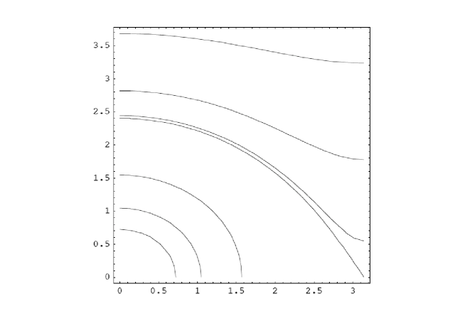
Figure 5: The lines of constant $\eta=0$ in the $x,y$ plane. The different curves correspond to $\tau=0.5,1,2,4,4.1,5,7$. These lines yield also the density $\rho(\tau,x)$. In order to get the density $\rho(\tau,\theta)$ we need the mapping between $x$ and $\theta$, which can be read on a figure like Fig. 4.

3.3 The curves of constant $\eta=0$

Because $\rho\sim y$, it is instructive to analyze the shape of the curves $\eta=0$ in the $(x,y)$ plane. Indeed this shape will be similar to that of the function $\rho(\theta)$, with $\theta$ related to $x$ as described in the caption of Fig. 4. Some curves $\eta=0$ are displayed in Fig. 5. These are determined by the implicit equation

$$y=\frac{\tau}{2}\,\frac{\sinh y}{\cosh y-\cos x}.$$ (35)

It is easy to show that the curves $\eta=0$ intersect the $y$-axis with a vanishing slope. Let us focus on their behavior near the $x$ axis. For small $y$ we have

$$y=\frac{\tau}{2}\frac{y}{1-\cos x},\qquad\cos x_{c}=1-\frac{\tau}{2}.$$ (36)

Thus, as long as $\tau\leq 4$, there is a value $x_{c}$ of $x$ at which the curve $\eta=0$ intersects the $x$-axis. As we shall verify later, this point is the singular point associated with the edge of the spectrum. In the vicinity of this point, the curve $\eta=0$ does not depend on $y$, that is, it has infinite slope in the $(x,y)$ plane.

For $\tau>4$, the curve intersects the axis $x=\pi$ at a point $y_{s}$ solution of

$$y_{s}=\frac{\tau}{2}\tanh\frac{y_{s}}{2}.$$ (37)

$y_{s}$ is a growing function of $\tau$. For large $\tau$, $y_{s}\simeq\pm\tau/2$, and one can easily construct the solution. Indeed we have then $\xi=\pi+iy_{s}\simeq\pi\pm i\tau/2$, so that

$$F_{0}(\xi)=\frac{1}{2}\cot\frac{\pi\mp i\tau/2}{2}=\pm\frac{i}{2}\tanh\frac{\tau}{2},$$ (38)

and the density is

$$\rho(\pi,\tau)=\frac{1}{2\pi}\tanh\frac{\tau}{2}.$$ (39)

For $\tau\to 4+0$, the equation for $y_{s}$ becomes

$$y_{s}=\frac{\tau}{2}\left(\frac{y}{2}-\frac{y^{3}}{24}\right),\qquad y_{s}^{2}\simeq 3(\tau-4),$$ (40)

so that

$$\rho(\pi,\tau)\simeq\frac{1}{4\pi}\sqrt{3(\tau-4)}.$$ (41)

Thus the derivative $\partial\rho/\partial\tau$ is singular at $\tau=4$.

3.4 The caustics

The construction of the solution of the Burgers equation from the characteristics is possible as long as the mapping between $\alpha$ and $\xi$ is one-to-one, that is, as long as $\partial\alpha/\partial\xi\neq 0$. When $\partial\alpha/\partial\xi=0$ a singularity develops. The equation which determines the location of the singularities is also that which determines the envelope of the characteristics, the so-called caustics of optics. Let $\xi_{c}(\tau)$ be the location of the singularity. We have

$$F_{0}^{\prime}(\xi_{c})=-\frac{1}{4\sin^{2}(\xi_{c}/2)}=-\frac{1}{\tau}.$$ (42)

The equation for the caustics is then given by

$$\alpha(\tau)=\xi_{c}(\tau)+\frac{\tau}{2}\cot\frac{\xi_{c}(\tau)}{2}.$$ (43)

By setting $\xi_{c}=x_{c}+iy_{c}$, we transform the singularity condition into two equations for $x_{c}$ and $y_{c}$:

$$\sinh(y_{c}/2)\,\cos(x_{c}/2) = 0$$

$$\cosh(y_{c}/2)\,\sin(x_{c}/2) = \pm\sqrt{\tau}/2.$$ (44)

These equations are equivalent to the equations $\partial_{x}\theta=\partial_{y}\theta=0$ (we used the Cauchy-Riemann conditions). The first equation implies that $y_{c}=0$ unless $x_{c}=\pi$. Consider the first possibility, i.e., $y_{c}=0$. The second equation then yields $\sin(x_{c}/2)=\pm\sqrt{\tau}/2$ which is possible only if $\tau\leq 4$. One concludes therefore that if $\tau>4$, $y_{c}\neq 0$ and $x_{c}=\pi$. Consider now the second possibility, $x_{c}=\pi$. In this case, the second equation yields $\cosh(y_{c}/2)=\pm\sqrt{\tau}/2$, which is possible only if $\tau\geq 4$. Therefore if $\tau<4$, $x_{c}\neq\pi$ and $y_{c}=0$. In summary, for $\tau<4$, the caustic lies in the plane $\eta=0$, while for $\tau>4$ it lies in the plane $\theta=\pi$.

For $\tau<4$, the value of $x_{c}$ is given by

$$x_{c}=2\arcsin({\sqrt{\tau}/2})=\arccos(1-\tau/2).$$ (45)

The equation of the caustics in the $\theta,\eta$ plane, is given by

$$\theta_{c}=2\arcsin({\sqrt{\tau}/2})+\sqrt{\tau(1-\tau/4)},\qquad\eta_{c}=0.$$ (46)

This is the curve plotted in Fig 2. The value $\theta_{c}$ corresponds also to the edge of the spectrum when $\tau\leq 4$. When the gap closes, $\tau\to 4$, $\theta_{c}\to\xi_{c}=\pi$.

For $\tau>4$, $y_{c}$ is given by

$$y_{c}=2{\rm argcosh}{\sqrt{\tau}/2},$$ (47)

and (for $y>0$)

$$\eta_{c}=2\,{\rm argcosh}{\sqrt{\tau}/2}-\sqrt{\tau(\tau/4-1)},$$ (48)

with $-\eta_{c}$ also solution (for $y<0$), describing a symmetric branch of the caustic. Note that as $\tau\to\infty$, $\eta_{c}\simeq-\tau/2$.

3.5 Solution of Burgers equation in the vicinity of the caustics

In the vicinity of the caustics one can construct the solution of the Burgers equation analytically. This is because one can then easily invert the relation between $\xi$ and $\alpha$. One has, quite generally,

$$F_{0}(\xi)=F_{0}(\xi_{c})+(\xi-\xi_{c})F_{0}^{\prime}(\xi_{c})+\frac{1}{2}(\xi-\xi_{c})^{2}F_{0}^{\prime\prime}(\xi_{c})+\frac{1}{6}(\xi-\xi_{c})^{3}F_{0}^{\prime\prime\prime}(\xi_{c})+\cdots,$$

so that

$$\alpha=\alpha_{c}+\frac{\tau}{2}(\xi-\xi_{c})^{2}F_{0}^{\prime\prime}(\xi_{c})+\frac{\tau}{6}(\xi-\xi_{c})^{3}F_{0}^{\prime\prime\prime}(\xi_{c})+\cdots$$ (50)

For $\tau\leq 4$, we have $\xi_{c}=2\arcsin({\sqrt{\tau}/2})$ and

$$\tau F_{0}(\xi_{c}) = \sqrt{\tau(1-\tau/4)},$$

$$\frac{\tau}{2}F^{\prime\prime}_{0}(\xi_{c}) = \sqrt{1/\tau-1/4},$$

$$\frac{\tau}{6}F^{\prime\prime\prime}_{0}(\xi_{c}) = -\frac{1}{3\tau}-\frac{2}{3}(1/\tau-1/4).$$ (51)

For $\tau<4$, one can ignore the cubic term. One gets then

$$\alpha=\alpha_{c}+(\xi-\xi_{c})^{2}\,\sqrt{1/\tau-1/4},$$ (52)

which is easily inverted to yield

$$\xi-\xi_{c}=\frac{\pm 1}{(1/\tau-1/4)^{1/4}}\sqrt{\alpha-\alpha_{c}}.$$ (53)

We have then

$$F(\alpha,\tau)=F_{0}(\xi(\alpha,\tau) \simeq F_{0}(\xi_{c})+(\xi-\xi_{c})F_{0}^{\prime}(\xi_{c})$$ (54)

$$= \sqrt{1/\tau-1/4}-\frac{1}{\tau}\frac{\sqrt{\alpha-\alpha_{c}(\tau)}}{(1/\tau-1/4)^{1/4}}.$$

The spectral density can be deduced from the imaginary part of $F$, or equivalently $F_{0}$.We have

$$\rho(\alpha)=\frac{1}{\pi}{\rm Im}F(\alpha-i0_{+}).$$ (55)

It follows that the spectral density vanishes for $\alpha>\alpha_{c}$ (confirming the interpretation of $\alpha_{c}$ as the edge of the spectrum). For $\alpha\mathrel{\hbox to0.0pt{\raise 2.20013pt\hbox{$<$}\hss}{\lower 2.20013pt\hbox{$\sim$}}}\alpha_{c}$,

$$\rho(\alpha)\simeq\frac{1}{\pi\tau(1/\tau-1/4)^{1/4}}\sqrt{\alpha_{c}-\alpha}\,.$$ (56)

When $\tau=4$, the second derivative vanishes, $\alpha_{c}=\pi=\xi_{c}$, and we have

$$\alpha=\pi-\frac{1}{3\tau}(\xi-\xi_{c})^{3},\qquad\alpha-\pi=-\frac{1}{3\tau}(\xi-\pi)^{3},$$ (57)

so that

$$\xi-\pi\simeq(3\tau)^{1/3}{\rm e}^{i\pi/3}(\alpha-\pi)^{1/3}.$$ (58)

It follows that the spectral density is given by (with $\alpha$ real and $\alpha<\pi$)

$$\rho(\alpha)\simeq\frac{(3\tau)^{1/3}}{\pi\tau}\sin\frac{\pi}{3}(\pi-\alpha)^{1/3}=\frac{1}{4\pi}\left(\frac{9\sqrt{3}}{2}\right)^{1/3}(\pi-\alpha)^{1/3}.$$ (59)

As $\tau$ grows beyond $\tau=4$, the real caustic splits into two complex ones, moving in opposite directions along the $\eta$ axis. At this point we shall not pursue our analysis with complex characteristics, but go through a specific study at $\theta=\pi$ using a different approach.

3.6 Specific study at $\theta=\pi$

In this section, we study the solution for $\theta=\pi$, using an approach which will allow us to make contact with the work of Neuberger [17, 18].

3.6.1 Solution with a real Burgers equation

Starting from the complex Burgers equation, for complex $\alpha$,

$$\partial_{\tau}F+\frac{1}{2}\partial_{\alpha}F^{2}=0,$$ (60)

we restrict $\alpha$ to $\alpha=\pi+i\eta=\pi-iy$ (where $y$ is the variable introduced by Neuberger). Choosing $y>0$, we get $\eta<0$ so that we are in the right domain of analyticity of $F$. In fact, $F$ is analytic except possibly at $y=0$ (where it develops a discontinuity when the gap closes; this discontinuity is proportional to the spectral density at $\alpha=\pi$). To avoid confusion (in all this discussion $x$ and $y$ will not have the same meaning as before in these lectures) we use Neuberger’s notation and set

$$\phi(y)=iF(\alpha=\pi-iy),\qquad\partial_{\tau}\phi(y,\tau)+\frac{1}{2}\partial_{y}\phi^{2}(y,\tau)=0,$$ (61)

with the boundary condition

$$\phi(y,\tau=0)=\phi_{0}(y)=-\frac{1}{2}\tanh\frac{y}{2}.$$ (62)

Note that since $F(\pi\mp i\epsilon)=\pm i\pi(\rho(\pi)$, we have

$$\rho(\pi,\tau)=\frac{1}{2\pi}\left[\phi(0_{-},\tau)-\phi(0_{+},\tau)\right].$$ (63)

3.6.2 Characteristics of the real Burgers equation

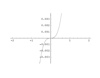
Figure 6: The function $f_{\tau}(x)$ plotted as a function of $x$ for the values $\tau=3,4,5$.

The characteristics are given by

$$y=x+\tau\phi_{0}(x)=x-\frac{\tau}{2}\tanh\frac{x}{2},$$ (64)

and the solution is given in terms of them by

$$\phi(y,\tau)=\phi_{0}(x(y,\tau)),\qquad x(y,\tau)=y-\tau\phi_{0}(x).$$ (65)

The velocity field $\phi(y,\tau)$ will eventually become infinitely steep at some points $y_{c}$. To determine these points we calculate the derivative $\partial_{y}\phi(y,\tau)$:

$$\frac{\partial\phi}{\partial y}=\frac{d\phi_{0}}{dx}\frac{dx}{dy}=\frac{d\phi_{0}}{dx}\frac{1}{dy/dx},$$ (66)

where we use the fact that $y$ and $x$ are related by the characteristic equation. It follows from this equation that

$$\frac{dy}{dx}=1+\tau\frac{d\phi_{0}}{dx}.$$ (67)

Since $d\phi_{0}/dx$ in Eq. (66) is finite for all $x$, an infinite slope in the velocity field will develop when $dy/dx=0$, that is, for values of $x_{c}$ such that

$$1+\tau\left.\frac{d\phi_{0}}{dx}\right|_{x_{c}}=0.$$ (68)

It is convenient to set

$$f_{\tau}(x)=\phi_{0}(x)+\frac{x}{\tau}.$$ (69)

The characteristic equation (64) reads then $y=\tau f_{\tau}(x)=0$, and the location of the singularities is given by $f^{\prime}(x_{c})=0$. The relation between $x$ and $y$ can be inverted if the solution of the equation $f_{\tau}(x)=y/\tau$ is unique. The plot in Fig. 6 indicates that this happens when $\tau<4$. Indeed the derivative of $f_{\tau}(x)$ is given by

$$f_{\tau}^{\prime}(x)=\frac{1}{\tau}-\frac{1}{4\cosh^{2}(x/2)},\qquad f^{\prime}_{\tau}(0)=\frac{1}{\tau}-\frac{1}{4},$$ (70)

so that the derivative in $x=0$ is positive as long as $\tau<4$. In this regime, there is a unique solution $x$ for each $y$. When $\tau=4$, $f^{\prime}(0)=0$, i.e., $x=0=x_{c}$ and the slope at $y=0$ of $\phi(y,4)$ is infinite. This is the preshock corresponding physically to the closure of the gap and the beginning of the build up of the spectral density at $\theta=\pi$. For $\tau>4$ the solution becomes multi-valued (takes an S-shape). The function $\phi$ becomes then discontinuous, its discontinuity giving the density, according to Eq. (63).

3.6.3 Solution of the real Burgers for large $\tau$

For large $\tau$, the solutions of the equation $f_{\tau}(x)=0$ are approximately given by

$$x_{1}=\frac{\tau}{2}\tanh\frac{\tau}{2}\;\;(x>0),\qquad x_{1}=-\frac{\tau}{2}\tanh\frac{\tau}{2}\;\;(x<0).$$ (71)

The solution of the characteristic equation $y=\tau f_{\tau}(x)$ are shifted linearly with respect to these values, when $y$ is small, that is, $\pm x_{1}\to\pm x_{1}+y$. It follows that $\phi(y,\tau)=(y-x_{1})/\tau$ becomes independent of $y$ in the vicinity of $y=0$, except for a jump that depends on the sign of $y$. We have

$$\phi(y<0,\tau)\simeq\frac{1}{2}\tanh\frac{\tau}{2},\qquad\phi(y>0,\tau)\simeq-\frac{1}{2}\tanh\frac{\tau}{2}.$$ (72)

It follows that

$$\rho(\pi,\tau)\simeq\frac{1}{2\pi}\tanh\frac{\tau}{2},$$ (73)

in agreement with Eq. (39).

3.6.4 Introducing a small viscosity

Anticipating on the discussion in the next sections, it is interesting to consider the viscid Burgers equation for $\phi(y,\tau)$

$$\partial_{\tau}\phi+\frac{1}{2}\partial_{y}\phi^{2}=\nu\partial_{y}^{2}\phi,$$ (74)

where $\nu$ plays the role of a viscosity (we shall see later that $\nu=1/2N_{c}$). This equation can be solved with the so-called Cole-Hopf transform

$$\phi(y,\tau)=-2\nu\partial_{y}\ln K(y,\tau),$$ (75)

where $K$ satisfies the diffusion equation

$$\frac{\partial K}{\partial\tau}=\nu\frac{\partial^{2}K}{\partial y^{2}}.$$ (76)

Let $K_{0}(x,\tau)$ be the solution that reduces to $\delta(x)$ at $\tau=0$:

$$K_{0}(x,\tau)=\frac{1}{\sqrt{4\pi\nu\tau}}{\rm e}^{-\frac{x^{2}}{4\nu\tau}}.$$ (77)

Then the solution of the Burgers equation reads

$$K(y,\tau)=\frac{1}{\sqrt{4\pi\nu\tau}}\int_{-\infty}^{+\infty}dx\,{\rm e}^{-\frac{(y-x)^{2}}{4\nu\tau}}{\rm e}^{-\frac{1}{2\nu}\int_{0}^{x}\phi_{0}(u)du}.$$ (78)

We have

$$\int_{0}^{x}du\,\phi_{0}(u)=-\ln\cosh\frac{x}{2},$$ (79)

and we can write

$$K(y,\tau)=\frac{1}{\sqrt{4\pi\nu\tau}}{\rm e}^{-\frac{y^{2}}{4\nu\tau}}\int_{-\infty}^{+\infty}dx\,{\rm e}^{-\frac{1}{2\nu}V(x)},$$ (80)

with

$$V(x)=\frac{x^{2}}{2\tau}-\frac{xy}{\tau}-\ln\cosh\frac{x}{2}\simeq\frac{x^{4}}{192}+\left(\frac{1}{\tau}-\frac{1}{4}\right)\frac{x^{2}}{2}-\frac{xy}{\tau}.$$ (81)

The expansion on the r.h.s. allows us to recover the Pearcey integral and study the vicinity of the critical point (near $\tau=4$) and the scaling with (small) viscosity. We have indeed

$$\int_{-\infty}^{+\infty}dx\,{\rm e}^{-\frac{1}{2\nu}V(x)}=4\left(\frac{3}{2}\right)^{1/4}\nu^{1/4}\int_{-\infty}^{+\infty}du\,{\rm e}^{-u^{4}-\alpha u^{2}+\xi u}$$ (82)

with

$$x=4\left(\frac{3}{2}\right)^{1/4}\nu^{1/4}u,$$ (83)

and the scaling variables related to $\tau$ and $y$ are, respectively

$$\alpha=4\left(\frac{3}{2}\right)^{1/2}\nu^{-1/2}\left(\frac{1}{\tau}-\frac{1}{4}\right),\qquad\xi=2\left(\frac{3}{2}\right)^{1/4}\nu^{-3/4}y.$$ (84)

4 The gapless phase and the inverse spectral cascade

In this section, we shall illustrate a particular feature of the disordered (gapless) phase. Consider the large $\tau$ uniform solution, and a small perturbation of the spectral density of the form

$$\rho(\theta,\tau_{0})=\frac{1}{2\pi}\left(1+2\epsilon\cos\theta\right)$$ (85)

with $\tau_{0}\gg 1$. Note that this form of the density results from truncating the general expansion (9) at the first moment, and set $w_{1}=\epsilon$. We wish to solve the Burgers equation with $\rho(\theta,\tau_{0})$ as the initial condition. The characteristics are given by

$$\theta=\xi+(\tau-\tau_{0})F_{0}(\xi),$$ (86)

and the function $F_{0}(\xi)$ corresponding to the initial condition can be read off Eq. (14):

$$F_{0}(\xi)=\frac{i}{2}\left(1+2\epsilon{\rm e}^{-i\xi}\right).$$ (87)

A singularity occurs for $\xi=\xi_{c}$, with $\xi_{c}$ solution of

$${\rm e}^{i\xi_{c}}=-\epsilon(\tau-\tau_{0}).$$ (88)

At $\xi_{c}$, we have

$$F_{0}(\xi_{c})=\frac{i}{2}-\frac{i}{\tau-\tau_{0}},\>\>F_{0}^{\prime}(\xi_{c})=-\frac{1}{\tau-\tau_{0}},\;\;F_{0}^{\prime\prime}(\xi_{c})=\frac{i}{\tau-\tau_{0}}.$$ (89)

We may now proceed and determine the solution in the vicinity of the singularity, as we did in Sect. 3. In the vicinity of the singularity we have

$$\theta=\theta_{c}+\frac{i}{2}(\xi-\xi_{c})^{2}.$$ (90)

The equation for the singularity, Eq. (88), has two solutions, depending on whether $\tau>\tau_{0}$ or $\tau<\tau_{0}$. Let us consider these solutions in turn.

If $\tau>\tau_{0}$,

$$\xi_{c}=\pi-i\ln\epsilon(\tau-\tau_{0})+2n\pi,$$ (91)

and

$$\theta_{c}=\pi-i\left(1-\frac{\tau-\tau_{0}}{2}+\ln\epsilon(\tau-\tau_{0})\right)$$ (92)

When $\tau$ is near $\tau_{0}$, $\tau\mathrel{\hbox to0.0pt{\raise 2.20013pt\hbox{$>$}\hss}{\lower 2.20013pt\hbox{$\sim$}}}\tau_{0}$, the singularity is at $\theta_{c}\sim\pi+i\infty$. As $\tau$ keeps increasing, $\theta_{c}$ remains complex unless $\epsilon$ is too large (i.e., unless $\epsilon\geq 1/2$). So, for small $\epsilon$, as one propagates forward in time, $\theta_{c}$ remains complex and return to $+i\infty$ as $\tau\to\infty$. Note that at large $\tau$, $F_{0}(\xi_{c})\sim i/2$ and the density $\rho\sim 1/2\pi$.

The situation is different for $\tau<\tau_{0}$. Then

$$\xi_{c}=-i\ln\epsilon(\tau_{0}-\tau)+2n\pi$$ (93)

and

$$\theta_{c}=-i\left(1+\frac{1}{2}(\tau_{0}-\tau)+\ln\epsilon(\tau_{0}-\tau)\right)$$ (94)

Again the singularity is at $+i\infty$ when $\tau=\tau_{0}$, but as $\tau$ decreases, it moves towards the real axis and reaches it in a finite time $\tau^{*}$ given by

$$0=1+\frac{1}{2}(\tau_{0}-\tau^{*})+\ln\epsilon(\tau_{0}-\tau^{*})$$ (95)

At this point we have the usual blow up, and the solution ceases to exist.

This simple calculation shows that while the complex Burgers equation provides a unique solution that connects the singular density at $\tau=0$ ($\rho(\theta)=\delta(\theta)$) and the uniform density at $\tau\to\infty$ ($\rho=1/2\pi$), this solution is “unstable” to backward motion for initial conditions that deviate only slightly form the generic solution of the Burgers equation. It is tempting to speculate that this particular feature is related to turbulent aspects of the disordered phase [19], and indeed the Burgers equation has often been used as a toy model to study such turbulent behavior. As a further remark, note that as one propagates forward in time, the higher moments of the spectral density are damped, leaving eventually only the uniform density at large time. This process is reminiscent of the inverse cascade, a feature of two-dimensional turbulence that can also be studied with the Burgers equation (for a pedagogical illustration of the phenomenon, see [20]).

5 Dyson fluid

In this section we would like to demystify somewhat the omnipresence of inviscid and viscid Burgers equations in the analysis of the closure of the spectral gap of Wilson loops. We will see that these equations originate from either algebraic or geometric random walks, where however the standard independent scalar increment is now replaced by its matrix-valued analogue. Actually, the idea of matrix-valued random walks appears already in pioneering papers on random matrix theories. In a classical paper [21], Dyson showed that the distribution of eigenvalues of a random matrix could be interpreted as the result of a random walk performed independently by each of the matrix elements. The equilibrium distribution yields the so-called “Coulomb gas” picture, with the eigenvalues identified to charged point particles repelling each other according to two-dimensional Coulomb law. For matrices of large sizes, this correctly describes the bulk properties of the spectrum [22]. In his original work, Dyson introduced a restoring force preventing the eigenvalues to spread for ever as time goes. This is what allowed him to find an equilibrium solution corresponding to the random ensemble considered with a chosen variance (related to the restoring force). We do not need to take this force into account here, since the phenomenon we are after is a non-equilibrium phenomenon. In particular, in the picture that we shall develop, and that we may refer to as “Dyson fluid”, the edge of the spectrum appears as the precursor of a shock wave, and its universal properties follow from a simple analysis of the Burgers equation that was developed in other contexts  [23]. This observation allows us to link familiar results of random matrix theory to universal properties of the solution of the Burgers equation in the vicinity of a shock [24].

5.1 Additive random walk of large matrices

We start from the simpler case of additive random walk of $N\times N$ hermitian matrices $H$ with complex entries. The explicit realization of the random walk is provided by the following construction: In the time step $\delta\tau$, $H_{ij}\to H_{ij}+\delta H_{ij}$, with $\langle\delta H_{ij}\rangle=0$, and $\langle(\delta H_{ij})^{2}\rangle=(1+\delta_{ij})\delta t,$ so at each time step, the increment of the matrix elements follows from a Gaussian distribution with a variance proportional to $\delta t$. The initial condition on the random walk is that at time $t=0$, all the matrix elements vanish. The crucial difference between the scalar and matricial random walk is visible when we switch from matrix elements to eigenvalues of $H$, which we denote by $x_{i}$. The random walk of the eigenvalues has the following characteristics [21]

$$\langle\delta x_{i}\rangle=E(x_{i})\,\delta t,\qquad\langle(\delta x_{i})^{2}\rangle=\delta t,$$ (96)

where the “Coulomb force”

$$E(x_{j})=\sum_{i\neq j}\left(\frac{1}{x_{j}-x_{i}}\right)$$ (97)

originates in the Jacobian $\Delta$ of the transformation from the matrix elements to the eigenvalues, $\Delta=\prod_{i<j}(x_{i}-x_{j})^{2}$. Note that now random walkers interact with each other, due to the “electric field” $E(x_{i}-x_{j})$. This interaction may a priori introduce non-linearities in the corresponding Smoluchowski-Fokker-Planck (SFP) equations. Indeed, this is the case, as we demonstrate below.

Using standard arguments, we see that the joint probability $P(x_{1},\cdots,x_{N},t)$ for finding the set of eigenvalues near the values $x_{1},\cdots,x_{N}$ at time $t$, obeys the SFP equation

$$\frac{\partial P}{\partial t}=\frac{1}{2}\sum_{i}\frac{\partial^{2}P}{\partial x_{i}^{2}}-\sum_{i}\frac{\partial}{\partial x_{i}}\left(E(x_{i})P\right).$$ (98)

The average density of eigenvalues, $\tilde{\rho}(x)$, may be obtained from $P$ by integrating over $N-1$ variables. Specifically:

$$\tilde{\rho}(x,t)=\int\prod_{k=1}^{N}dx_{k}\,P(x_{1},\cdots,x_{N},t)\sum_{l=1}^{N}\delta(x-x_{l}),$$ (99)

with normalization $\int dx\,\tilde{\rho}(x)=N.$ Similarly we define the “two-particle” density $\tilde{\rho}(x,y)=\langle\sum_{l=1}^{N}\sum_{j\neq l}\delta(x-x_{l})\delta(y-x_{j})\rangle,$ with $\int dx\,dy\,\tilde{\rho}(x,y)=N(N-1).$ These various densities obey an infinite hierarchy of equations obtained form Eq. (98) for $P$. Thus, the equation relating the one and two particle densities reads

$$\frac{\partial\tilde{\rho}(x,t)}{\partial t}=\frac{1}{2}\frac{\partial^{2}\tilde{\rho}(x,t)}{\partial x^{2}}-\frac{\partial}{\partial x}\fint dy\,\frac{\tilde{\rho}(x,y,t)}{x-y},$$ (100)

where $\fint$ denotes the principal value of the integral.

In the large $N$ limit, this equation becomes a closed equation for the one particle density. To show that, we set

$$\tilde{\rho}(x,y)=\tilde{\rho}(x)\tilde{\rho}(y)+\tilde{\rho}_{con}(x,y),$$ (101)

where $\tilde{\rho}_{con}(x,y)$ is the connected part of the two-point density. Then we change the normalization of the single particle density, defining

$$\tilde{\rho}(x)=N\rho(x),$$ (102)

and similarly $\tilde{\rho}(x,y)=N(N-1)\,\rho(x,y)$. At the same time, we rescale the time so that $\tau=Nt$ [25]. One then obtains

$$\frac{\partial\rho(x)}{\partial\tau}\!+\!\frac{\partial}{\partial x}\rho(x)\!\fint\!dy\,\frac{\rho(y)}{x-y}=\frac{1}{2N}\frac{\partial^{2}\rho(x)}{\partial x^{2}}\!+\!\fint dy\,\frac{\rho_{con}(x,y)}{x-y}.$$

In the large $N$ limit, the right hand side vanishes, leaving as announced a closed equation for $\rho(x,\tau)$. Taking the Hilbert transform of the above equation, and following the procedure from the previous sections, we immediately recognize the complex inviscid Burgers equation for the resolvent

$$G(z,\tau)=\left<\frac{1}{N}{\rm Tr}\frac{1}{z-H(\tau)}\right>=\int dy\,\frac{\rho(y,\tau)}{z-y},$$ (104)

which reads explicitly

$$\partial_{\tau}G(z,\tau)+G(z,\tau)\,\partial_{z}G(z,\tau)=0.$$ (105)

Let us comment the differences between this equation and the standard diffusion: First, the usual Laplace term $(1/2)\Delta$ has vanished, since in the matricial case this term is dwarfed by $1/N$ factor. An additional non-linear term has however appeared, due to the interaction of diffusing eigenvalues, a term which by definition is absent in a one-dimensional random walk. This is how the inviscid (complex) Burgers equation [8, 25] appears in the matrix-valued diffusion process. The resulting nonlinearity can trigger shock waves, as we will see below.

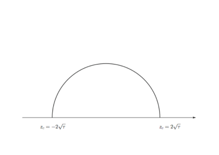
Figure 7: The Wigner semi-circle.

Repeating the method of (complex) characteristics described in Sect. 3, with the characteristics determined by the implicit equation

$$z=\xi+\tau G_{0}(\xi),\qquad G_{0}(z)=G(z,\tau=0)=1/z.$$ (106)

and assuming the solution $\xi(z,\tau)$ to be known, the Burgers equation can be solved parametrically as $G(z,\tau)=G_{0}(\xi(z,\tau))=G_{0}(z-\tau G(z,\tau))$. The solution of this equation that is analytic in the lower half plane is

$$G(z,\tau)=\frac{1}{2\tau}(z-\sqrt{z^{2}-4\tau})\,,$$ (107)

whose imaginary part yields the familiar Wigner’s semicircle for the average density of eigenvalues. This is perhaps the fastest, and quite intuitive, derivation of this seminal result.

In the fluid dynamical picture suggested by the Burgers equation, the edge of the spectrum corresponds to a singularity that is associated with the precursor of a shock wave, sometimes referred to as a “pre-shock”  [23]. As discussed earlier, this singularity occurs when

$$dz/d\xi=0=1+\tau G^{\prime}_{0}(\xi_{c}),$$ (108)

defining $\xi_{c}(\tau)$. Since $G_{0}^{\prime}(\xi_{c})=-1/\xi_{c}^{2}$, $\xi_{c}(\tau)=\pm\sqrt{\tau}$, and

$$z_{c}=\xi_{c}+\tau G_{0}(\xi_{c})=\pm 2\sqrt{\tau}.$$ (109)

That is, the singularity occurs precisely at the edge of the spectrum, traveling with time $\tau$. Furthermore, the resulting singularity is of the square root type. To see that, one expands the characteristic equation around the singular point. One gets

$$z-z_{c}=\frac{\tau}{2}(\xi-\xi_{c})^{2}G_{0}^{\prime\prime}(\xi_{c})=\frac{\tau}{\xi_{c}^{3}}(\xi-\xi_{c})^{2}.$$ (110)

It follows that, in the vicinity of the positive edge of the spectrum $z\simeq z_{c}=2\sqrt{\tau}$,

$$\xi-\xi_{c}=\pm\tau^{1/4}\sqrt{z-z_{c}}.$$ (111)

Thus, as $z$ moves towards $z_{c}$ and is bigger than $z_{c}$, $\xi$ moves to $\xi_{c}$ on the real axis. When $z$ becomes smaller than $z_{c}$, $\xi$ moves away from $\xi_{c}$ along the imaginary axis. The imaginary part therefore exists for $z<z_{c}$ and yields a spectral density $\rho(z)\sim\sqrt{z_{c}-z}$, in agreement with (107). This square root behavior of the spectral density implies that in the vicinity of the edge of the spectrum, the number of eigenvalues in an interval of width $s$ scales as $Ns^{3/2}=(N^{2/3}s)^{3/2}$, implying that the interlevel spacing goes as $N^{-2/3}$.

This scaling of the preshock wave resembles the Airy scaling in random matrix models. Indeed, we can provide a rigorous argument why this is the case [24]. Note that in the case of an additive diffusion we can simply find the solution of Eq. (98)

$$P(x_{1},\cdots,x_{N},t)=C\prod_{i<j}(x_{i}-x_{j})^{2}\,{\rm e}^{-\sum_{i}\frac{x_{i}^{2}}{2t}},$$ (112)

with $C$ a (time-dependent) normalization constant. Indeed, in the random walk described above, the probability distribution retains its form at all instants of time. This means that we can repeat the standard stationary solution in terms of time dependent Hermite polynomials, which now remain orthogonal with respect to the time-dependent measure $\exp\left(-Nx^{2}/(2\tau)\right)$. Explicitly, the monic, time-dependent orthogonal Hermite polynomials read

$$\pi_{k}(x,\tau)=\frac{(-i)^{k}}{k!}\sqrt{\frac{N}{2\pi\tau}}\!\int dqq^{k}e^{-\frac{N}{2\tau}(q-ix)^{2}},$$ (113)

and satisfy

$$\int_{-\infty}^{\infty}{dx}{\rm e}^{-\frac{Nx^{2}}{2\tau}}\pi_{n}(x,\tau)\pi_{m}(x,\tau)=\delta_{nm}c_{n}^{2},$$ (114)

with $c_{n}^{2}=n!\sqrt{2\pi}\tau^{n+1/2}$, where we have used conventions from [26]. Note that the monic character of the $\pi_{n}$’s is not affected by the time dependence.

By using the integral representation (113), it is easy to show that the $\pi_{n}(x,\tau)$’s satisfy the following equation

$$\partial_{\tau}\pi_{n}(x,\tau)=-\nu_{s}\partial_{x}^{2}\pi_{n}(x,\tau),$$ (115)

with $\nu_{s}={1}/{2N}$, for any finite $N$. This is a diffusion equation with, however, a negative diffusion constant, which prevents an immediate physical interpretation. One can however understand intuitively this negative sign: a positive diffusion (viscosity) would smoothen the shock wave. In order to obtain the wildly oscillating pattern of the preshock corresponding to the universal spectral fluctuations in the random matrix theory, we need an opposite mechanism. Note also that $\pi_{n}$ is an analytic function of $x$, and $\pi_{n}(-iy,\tau)$, with $y$ real, satisfies a diffusion equation with a positive constant.

As a last step, to see the emerging viscid Burgers structure, we perform a so-called inverse Cole-Hopf transform, i.e., we define the new function

$$f_{k}(z,\tau)\equiv 2\nu_{s}\partial_{z}\ln\pi_{k}(z,\tau)=\frac{1}{N}\sum_{i=1}^{k}\frac{1}{z-\bar{x}_{i}(\tau)},$$ (116)

with ${\rm Im}z\neq 0$. The resulting equation for $f_{k}$ is the viscid Burgers [15] equation

$$\partial_{\tau}f_{k}(z,\tau)+f_{k}(z,\tau)\partial_{z}f_{k}(z,\tau)=-\nu_{s}\partial_{z}^{2}f_{k}(z,\tau).$$ (117)

The equation (117) is satisfied by all the functions $f_{k}$, for any $k$. We shall focus now on the function $f_{N}$ associated to $\pi_{N}(z,\tau)$, due to the known fact that $\pi_{N}(z,\tau)$ is equal to the average characteristic polynomial [29], i.e

$$\left<\det(z-H(\tau))\right>=\pi_{N}(z,\tau).$$ (118)

Note that in the large $N$ limit, $\partial_{z}\ln\langle\det(z-H(\tau))\rangle\approx\partial_{z}\langle\ln\det(z-H(\tau))\rangle=N\,G(z)$. Thus $f_{N}(z,\tau)$ coincides with the average resolvent $G(z,\tau)$ in the large $N$ limit. In fact the structure of $f_{N}$, as clear from Eq. (116), is very close to that of the resolvent, with its poles given by the zeros of the characteristic polynomial. Eq. (117) for $f_{N}(z,\tau)$ is exact. The initial condition, $f_{N}(z,\tau=0)=1/z$, does not depend on $N$, so that all the finite $N$ corrections are taken into account by the viscous term. This observation allows us to recover celebrated Airy universality in the random matrix models, this time solely from the perspective of the theory of turbulence [27]. Let us recall that in the vicinity of the edge of the spectrum, and in the inviscid limit,

$$f_{N}(z,\tau)\simeq\pm\frac{1}{\sqrt{\tau}}\mp\frac{1}{\tau^{3/4}}\sqrt{z-z_{c}}.$$ (119)

We set

$$x=z_{c}(\tau)+\nu_{s}^{2/3}s,\quad f_{N}(x,\tau)=\dot{z}_{c}(\tau)+\nu_{s}^{1/3}\chi_{N}(s,\tau),$$ (120)

with $\dot{z}_{c}\equiv\partial_{\tau}z_{c}=\pm 1/\sqrt{\tau}$. The particular scaling of the coordinate is motivated by the fact that near the square root singularity the spacing between the eigenvalues scales as $N^{-2/3}$. A simple calculation then yields the following equation for $\chi(s,\tau)$ in the vicinity of $z_{c}(\tau)=2\sqrt{\tau}$:

$$\partial_{\tau}^{2}z_{c}+\nu_{s}^{1/3}\frac{\partial\chi}{\partial\tau}+\chi\frac{\partial\chi}{\partial s}=-\frac{\partial^{2}\chi}{\partial s^{2}},$$ (121)

which, ignoring the small term of order $\nu_{s}^{1/3}$, we can write as

$$\frac{\partial}{\partial s}\left[-\frac{s}{2\tau^{3/2}}+\frac{1}{2}\chi^{2}+\frac{\partial\chi}{\partial s}\right]=0.$$ (122)

Note that the expression in the square brackets represents the Riccati equation, so the particular explicit solution corresponding to characteristic polynomial is

$$\chi(s,\tau)=2\frac{Ai^{\prime}(a^{1/3}(s))}{Ai(a^{1/3}(s))}.$$ (123)

where $Ai$ denotes the Airy function, and $a=1/(4\tau)^{3/2}$.

For completeness we note, that the Cauchy transforms of the monic orthogonal polynomials

$$p_{k}(z,\tau)=\frac{1}{2\pi i}\int_{-\infty}^{\infty}dx\frac{\pi_{k}(x,\tau)e^{-Nx^{2}/2\tau}}{x-z},$$ (124)

which are related to average inverse spectral determinant, generate similar universal preshock phenomena in complex Burgers equations. Their detailed behavior in the vicinity of the preshock is related to the two remaining solutions of the Airy equation (Airy of the second kind, [28]).

5.2 Multiplicative random walk of large matrices

The case of multiplicative (geometric) one dimensional random walk can be easily reduced to the additive one, since $e^{x+y}=e^{x}e^{y}$, so taking the logarithm of the multiplicative random walk reduces this case to the additive random walk of the logarithms of multiplicative increments. Note that this simple prescription does not work in the case of matrices. First, the product of two hermitian matrices is no longer hermitian, second, matrices do not commute, so $e^{X+Y}\neq e^{X}e^{Y}$. This means that the matrix-valued geometric random walk may exhibit new and interesting phenomena. To avoid the nonhermiticity of the product of hermitian matrices, we stick to unitary matrices - their product is unitary and a simple realization is

$$U=\exp\{i\sqrt{\delta t}H\}$$ (125)

where $H$ is hermitian. Note that this procedure is equivalent to Janik-Wieczorek model, described in the first part of these notes. Following Dyson, we recover that the only difference corresponding to the multiplicative case is the modification of the electric force. Since the eigenvalues of the unitary matrices are forced to stay on the unit circle, the electric force has to respect periodicity, i.e. has to gain contributions from all the distances between the interacting charges modulo $2\pi m$, where $m$ is the integer. This infinite resummation modifies the electric force, yielding a SFP equation for Circular Unitary Ensemble [21] and corresponding to the process where

$$\langle\delta y_{i}\rangle=E(y_{i})\,\Delta t,\qquad\langle(\delta y_{i})^{2}\rangle=\Delta t,$$ (126)

where $E(y_{i})=\frac{1}{2}\sum_{i\neq j}\cot(y_{i}-y_{j})/2$, parameterizing the eigenvalues on the unit circle as $z=\exp(iy)$. This particular form of the electric field was already met in the first part of these lectures. Let us make two remarks. First, we note that in the present case, in order to reach the equilibrium solution, corresponding to a uniform distribution of eigenvalues along the unit circle, one does not need the stabilizing external force – due to the compactness of the support of the eigenvalues the mutual repulsion between them is sufficient to reach equilibrium in the infinite time limit. Second, we may expect a new universal phenomenon – due to the compactness of the support of the spectrum, left and right Airy preshocks at the ends of evolving packet of eigenvalues have to meet at some critical time, creating universal generalized Airy function exhibiting novel scaling with large $N$.

In principle, we can follow the route sketched above for the additive case, i.e. find the time-dependent solution of the pertinent SFP equation and construct orthogonal polynomials. This time however the mathematics is more involved – the time dependent solution does not factorize nicely, and depends on the ratio of Vandermonde determinants built from Jacobi theta functions (solutions of diffusion equation with periodic boundary conditions), and the corresponding orthogonal polynomials belong to Schur class. In order to avoid these complications and to make connection with the lectures of H. Neuberger [30] at this School, we make the following observation [31]. Let us define a generic observable

$$\e^{-a\tau}O(z,U)\equiv e^{-a\tau}\sum_{R}\frac{a_{r}(z)}{d_{R}}\chi_{R}(U^{\dagger}),$$ (127)

where the sum is over the representations, $\chi_{R}$ denotes the character of the representation $R$ and $d_{R}$ its dimension. Calculating the expectation value of the above object with respect to the measure [30]

$$P(U)=\sum_{R}d_{R}\,\chi_{R}(U)e^{-\tau C_{2}(R)},$$ (128)

where $C_{2}(R)$ is a Casimir operator for the representation $R$, we get

$$\left<e^{-a\tau}O(z,U)\right>=e^{-a\tau}\sum_{R}a_{R}(z)\,e^{-\tau C_{2}(R)}.$$ (129)

If we act now on this expression with the heat-kernel operator $(z\partial_{z})^{2}+\kappa\partial_{\tau}$, we notice that the heat equation does not mix the coefficients $a_{R}$ corresponding to different representations. This allows us to write down a simple solution

$$a_{R}(z)=z^{\pm\sqrt{\kappa(C_{2}(R)+a)}}.$$ (130)

This expression has to be well defined on the unit circle, which implies that the argument of the square root has to be the square of an integer. This imposes very strong restriction on Young diagrams forming the representation $R$. For antisymmetric representations considered in Ref. [17], the single valued-ness of the solution corresponds to $a=-N/8$, provided the evolution time is identified as $\tau=t(1+{1}/{N})$. Indeed, the combination of Casimir and $a$ reads in this case $\frac{1}{2N}\left(\frac{N}{2}-k\right)^{2}$, for any $k$ running between $0$ and $N$. This gives the whole family of $(N+1)$ heat equations, one for each $k$, in analogy to the family of monic Hermite polynomials fulfilling the heat equation for the case of additive random walk. Since the heat equation is linear, any combination of monomials in $z$ fulfills the same equation. In particular this is the case of the characteristic polynomial considered by Neuberger [17]. As before, the inverse Cole-Hopf transformation yields the viscid Burgers equation. Note that this construction explains naturally the appearance of the somewhat mysterious extra factor $e^{-N\tau/8}$ in the corresponding viscid Burgers equations for the characteristic polynomial. For completeness we note that a similar viscid Burgers structure appears for the inverse characteristic polynomial [18]. Now, the relevant representations are symmetric, which corresponds to “time” $\tau=t(1-\frac{1}{N}),$ and unrestricted $k$ running from zero to infinity, and the argument of the square root is proportional to $(\frac{N}{2}+k)^{2}$, provided that again $a=-N/8$. This gives the infinite hierarchy of heat equations for any $k$. Since $1/\det(z-U)$ can be expanded into infinite series in $1/z$, again the pertinent inverse Cole-Hopf transformation reproduces viscid complex Burgers equation, as noted by Neuberger.

Alike in the additive case, we can now analyze the critical behavior at the closure of the spectral gap, using the tools of the theory of turbulence for the coalescence of two Airy-like universal preshocks merging at $z=-1$ at some critical time. However, instead of going into the beautiful, but involved mathematical construction corresponding to the appearance of the universal Pearcey function at the closure of the gap, we propose to exploit a somewhat unexpected analogy between the spectral properties of the gap in large $N_{c}$ Yang-Mills theory and geometric optics.

6 Diffraction catastrophes and large $N$ universalities in YM theories

The large $N$ limit is very often considered as a “classical” one, since it switches off fluctuations. In the spirit of this analogy we consider classical (geometric) optics, where the wavelength vanishes, $\lambda=0$, and rays of light are straight lines. These rays of light can condense on some surfaces, yielding high intensity (actually, in the $\lambda=0$ limit infinite intensity) hypersurfaces, which are called caustics, from a Greek word denoting “burning”. If we relax the restrictions of geometric optics, i.e., if we allow for some very small $\lambda\neq 0$, wave patterns of light appear. Rays start to interfere, forming wave packets, and intensity is no longer infinite. We may ask now, how the limiting procedure from wave optics to geometric optics takes place. In other words, we ask how the wave packet scales with $\lambda\rightarrow 0$. The answer to this intriguing question has been provided by Berry and Howls [32], and their classification of “color diffraction catastrophes” is a particular, physical realization of the classification of singularities in the so-called catastrophe theory. There are only seven stable caustics, the two lowest, relevant for our analysis, corresponding to so-called fold and cusp singularities, controlled by one and two parameters, respectively . The scaling of the wave packet in these two cases reads [35]

$$\Psi(\vec{r},\lambda)\sim\frac{1}{\lambda^{\beta}}\psi\left(\frac{x}{\lambda^{\sigma_{1}}},\frac{y}{\lambda^{\sigma_{2}}}\right)$$ (131)

where $\vec{r}$ denotes a set of “control parameters” and the universal critical exponents $\sigma_{i}$ and $\beta$ are known respectively as Berry and Arnold indices. The Table 1. summarizes the universal properties of caustics.

Type	$\beta$	$\sigma_{i}$	$\psi$
Fold	$\beta=\frac{1}{6}$	$\sigma=\frac{2}{3}$	$\psi=2\pi Ai(\xi)=\int_{-\infty}^{\infty}dt\exp i(t^{3}/3+\xi t)$
Cusp	$\beta=\frac{1}{4}$	$\sigma_{x}=\frac{1}{2}\,\,\,\,\,\sigma_{y}=\frac{3}{4}$	$\psi=P(\xi,\eta)=\int_{-\infty}^{\infty}dt\exp i(t^{4}/t+\xi t^{2}/2+\eta t)$

Table 1: Classification of two lowest stable singularities

Immediately we see an analogy between the Airy ($Ai(\xi)$) and Pearcey ($P(\xi,\eta)$) universal functions appearing at the fold and cusp ( merging of two folds) and which describe the properties of the characteristic polynomials for critical spectra of Wilson loops in Yang-Mills theory, also for $D>2$. Complex characteristics (straight lines) play the role of rays of line. Singularities (shock waves) correspond to caustics, finite viscosity ($1/2N$) scaling has the same critical indices as finite $\lambda$ scaling for the intensity of the wave packets, see Eqs.(82)-(84). The exact correspondence is summarized in the form of the Table 2.

GEOMETRIC OPTICS	$N=\infty$ YANG-MILLS
wavelength $\lambda=0$	viscosity $\nu_{s}=\frac{1}{2N}=0$
rays of light	rays of characteristics
caustics	singularities of Wilson loop spectra
WAVE OPTICS	FINITE $N$ YANG-MILLS
$\Psi(\vec{r},\lambda)\sim\frac{1}{\lambda^{\beta}}\psi(\frac{x}{\lambda^{\sigma_{1}}},\frac{y}{\lambda^{\sigma_{2}}})$	$<\det(z-W(C))>$
Fold scaling $\sigma=2/3$	$N^{2/3}$ scaling at the edge
Cusp scaling $\sigma_{1}=1/2\,\,\,\sigma_{2}=3/4$	$N^{1/2}$ and $N^{3/4}$ scaling at critical size

Table 2: Morphology of singularities – analogies.

We find it rather intriguing that the beautiful scaling of interference fringes in diffractive optics could belong to the same universality class as the finite $N$ critical scaling of the spectral density of the Wilson operator in non-Abelian gauge theories in nontrivial dimensions.

7 Outlook

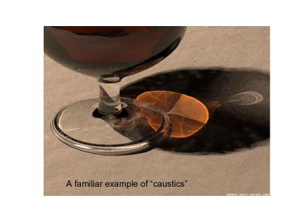
Figure 8: A familiar example of caustics [33]. Note two fold-line caustics merging into the cusp.

In these lectures, we have shown how the study of the complex Burgers equation sheds a new light on universal properties of the the large $N_{c}$ transition in multicolor Yang-Mills, that was first identified by Durhuus and Olesen many years ago. These lectures should be viewed as complementary to those by Neuberger and by Narayanan at this School, and they offer a view of a similar subject from different angles and perspectives. Our observations allow us to link together domains of theoretical physics and mathematics that are rather unrelated at first sight: The spectral flow of eigenvalues of the Wilson operators has features reminiscent of classical turbulence, the universal behavior is locked by multiplicative unitary diffusion considered by Dyson already in 1962, critical exponents belong to a classification of stable singularities (catastrophe theory) and the phenomenon of scaling with finite $N$ at critical size of the Wilson loop has exact counterpart in diffractive optics! The fact the whole dynamics of complicated non-perturbative QCD can be reduced in some spectral regime to a matrix model is not new - a notable case is the universal scaling of the spectral density of the Euclidean Dirac operator for sufficiently small eigenvalues, where the spectrum belongs to the broad universality class of the corresponding chiral models [36]. What we find remarkable is that, in the case of the large $N_{c}$ transition, the analogous universal matrix model seems to be represented by the simplest realization of the multiplicative matrix random walk. In general, one may expect that in a very narrow spectral window around $\lambda=-1$ a universal oscillatory behavior appears as a preparation for the formation of the spectral shock-wave, in qualitative analogy to similar spectral oscillations of quark condensate before spontaneous breakdown of the chiral symmetry based on Banks-Casher relation [37].

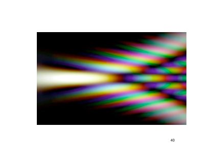
Figure 9: Color diffraction catastrophe [34]. Picture shows modulus of Pearcey function, anisotropic character of interference fringes reflects different scaling exponents $\sigma_{1}$ and $\sigma_{2}$.

Certainly, further generalizations and analogies are possible. We mention here the extension to supersymmetric models, intriguing role of the fermions [38] and the analogies with shock phenomena in mezoscopic systems (universal conductance fluctuations) [39] or growth processes of the Kardar-Parisi-Zhang universality class and statistical properties of the equilibrium shapes of crystals [40]. We hope that these lectures will trigger the need of better understanding of all these relations and analogies.

8 Acknowledgements

We thank R. Narayanan and H. Neuberger for several discussions and private correspondence. We also benefited from illuminated remarks by R.A. Janik and R. Speicher. This work was supported in part by Polish Ministry of Science Grant No. N N202 229137 (2009-2012).

References

- [1] G. ’tHooft, Nucl. Phys. B 72 (1974) 461.
- [2] E. Witten, Nucl. Phys. B 160 (1979) 57.
- [3] B. Durhuus and P. Olesen, Nucl. Phys. B184 (1981) 406; Nucl. Phys. B184 (1981) 461.
- [4] Yu. Makeenko and A.A. Migdal, Phys. Lett 88B (1979) 135.
- [5] R. Narayanan and H. Neuberger, [hep-th] 0711.4551
- [6] R. A. Janik and W. Wieczorek, J. Phys. A: Math. Gen. 37 (2004) 6521.
- [7] E. Gudowska-Nowak, R. A. Janik, J. Jurkiewicz and M. A. Nowak, Nucl. Phys. B670 (2003) 479; New Jour. of Phys. 7 (2005) 54.
- [8] D. V. Voiculescu, K. J. Dykema and A. Nica, Free Random Variables, CRM Monograph Series, Vol.1, Am. Math. Soc., Providence, 1992.
- [9] R. Speicher, Math. Ann. 298 (1994) 611.
- [10] The exact correspondence between JW model and YM2 was observed by M.A. Nowak, P. Olesen and perhaps several others.
- [11] V.A. Kazakov and I.K. Kostov, Nucl. Phys. B176 (1980) 199; P. Rossi, Annals Phys. 132 (1981) 463; A. Basetto, L. Griguolo and F. Vian, Nucl. Phys. 559 (1999) 563.
- [12] D. Gross and A. Matytsin, Nucl. Phys. B429 (1994) 50; Nucl. Phys. B437 (1995) 541.
- [13] P. Olesen, Nucl. Phys. B559 (1999) 197;[hep-th] 0712.0923.
- [14] R. Gopakumar and D. Gross, Nucl. Phys. B 451 (1995) 379 and references therein.
- [15] J.M. Burgers, The Nonlinear diffusion equation, D. Reidel Publishing Company (1974).
- [16] P. Constantin, A. J. Majda and E. Tabak, Nonlinearity 7 (1994) 1495.
- [17] H. Neuberger, Phys. Lett. B666 (2008) 106.
- [18] H. Neuberger, Phys. Lett. B670 (2008) 235.
- [19] J.-P. Blaizot and M.A. Nowak, Phys. Rev. Lett. 101 (2008)100102.
- [20] W. I. Newman, Chaos, vol 10, no2, 393 (2000).
- [21] F.J. Dyson, J. Math. Phys. 3 (1962) 1191.
- [22] For a review, see T. Guhr, A. Mueller-Groeling and H.A. Weidenmueller, Phys. Rept. 299 (1998) 189.
- [23] D. Bessis and J.D. Fournier, J. Physique Lett. 45 (1984) L833.
- [24] J.-P. Blaizot and M.A. Nowak, hep-th/0902.2223.
- [25] P. Biane and R. Speicher, Ann. Inst. H. Poincaré PR 37 (2001) 581.
- [26] Y. V. Fyodorov, e-print math-ph/0412017.
- [27] S.J. Chapman, C.J. Howls, J.R. King and A.B. Olde Daalhuis, Nonlinearity, 20 (2007) 2425.
- [28] O. Vallee and M. Soares, Airy functions and applications to physics, Imperial College Press, 2004.
- [29] E. Brezin and S. Hikami, Commun. Math. Phys. 214 (2000) 111.
- [30] H. Neuberger, hep-th/0906.5299.
- [31] J.-P. Blaizot, R.A. Janik and M.A. Nowak, in preparation.
- [32] M. Berry, Les Houches Lectures Series LII (1989), ed. M.-J. Giannoni, A. Voros and J. Zinn-Justin, North Holland, Amsterdam (1991), pp.251-304 and references therein.
-
[33]
This picture by Henrik Wann Jensen can be found at http://graphics.ucsd.edu/
~henrik/images/caustics.html - [34] This picture of cusp catastrophe comes from gallery of Sir M. V. Berry, http://www.phy.bris.ac.uk/people/berry_ mv/gallery.html
- [35] M.V. Berry and S. Klein, Proc. Natl. Acad. Sci. USA 93 (1996) 261.
- [36] J.J.M. Verbaarschot and I. Zahed, Phys. Rev. Lett. 70 (1993) 3852; J.J.M. Verbaarschot Phys. Rev. Lett. 80 (1998) 1146.
- [37] T. Banks and A. Casher, Nucl. Phys. B169 (1980) 103.
- [38] R. Narayanan and H. Neuberger, hep-th/0909.4066.
- [39] C.W.J. Beenakker, Rev. Mod. Phys. 69 (1997) 731.
- [40] H. Spohn, e-print cond-mat/0512011.