Strongly coupled Skyrme-Faddeev-Niemi hopfions

Abstract

The strongly coupled limit of the Skyrme-Faddeev-Niemi model (i.e., without quadratic kinetic term) with a potential is considered on the spacetime $\mathbb{S}^{3}\times\mathbb{R}$. For one-vacuum potentials two types of exact Hopf solitons are obtained. Depending on the value of the Hopf index, we find compact or non-compact hopfions. The compact hopfions saturate a Bogomolny bound and lead to a fractional energy-charge formula $E\sim|Q|^{1/2}$, whereas the non-compact solitons do not saturate the bound and give $E\sim|Q|$. In the case of potentials with two vacua compact shell-like hopfions are derived.
Some remarks on the influence of the potential on topological solutions in the full Skyrme-Faddeev-Niemi model or in (3+1) Minkowski space are also made.

1 Introduction

The Skyrme-Faddeev-Niemi (SFN) model [1], [2] is a field theory with hopfions as solitonic excitations. The model is given by the following Lagrange density

$$L=\alpha(\partial_{\mu}\vec{n})^{2}-\beta[\partial_{\mu}\vec{n}\times\partial_{\nu}\vec{n}]^{2}-\lambda V(\vec{n}),$$ (1)

where $\vec{n}=(n^{1},n^{2},n^{3})$ is a unit iso-vector living in $(3+1)$ dimensional Minkowski space-time. Additionally, $\alpha,\beta,\lambda$ are positive constants. The second term, referred to as the Skyrme term (strictly speaking the Skyrme term restricted to $\mathbb{S}^{2}$) is obligatory in the case of 3 space dimensions to avoid the Derrick argument for the non-existence of static, finite energy solutions. The requirement of finiteness of the energy for static configurations leads to the asymptotic condition $\vec{n}\rightarrow\vec{n}_{0}$, as $\vec{x}\rightarrow\infty$, where $\vec{n}_{0}$ is a constant vector. Thus, static configurations are maps $\mathbb{R}^{3}\cup\{\infty\}\cong\mathbb{S}^{3}\rightarrow\mathbb{S}^{2}$ and therefore can be classified by the pertinent topological charge, i.e., the Hopf index $Q\in\pi_{3}(\mathbb{S}^{2})\cong\mathbb{Z}$. Moreover, as the pre-image of a fixed $\vec{n}\in\mathbb{S}^{2}$ is isomorphic to $\mathbb{S}^{1}$, the position of the core of a soliton (pre-image of the antipodal point $-\vec{n}_{0}$) forms a closed, in general knotted, loop. For a recent detailed review of the SFN model and related models which support knot solitons we refer to [3].
The physical interest of the SFN model is related to the fact that it may be applied to several important physical systems. In the context of condensed matter physics, it has been used to describe possible knotted solitons for multi-component superconductors [4], [5]. In field theory, its importance originates in the attempts to relate it to the low energy (non-perturbative), pure gluonic sector of QCD [1], [6]. In this picture, relevant particle excitations, i.e., glueballs are identified with knotted topological solitons. This idea is in agreement with the standard picture of mesons, where quarks are connected by a very thin tube of the gauge field. Now, because of the fact that glueballs do not consist of quarks, such a flux-tube cannot end on sources. In order to form a stable object, the ends must be joined, leading to loop-like configurations.
Although the SFN model (or some generalization thereof) might provide the chance for a very elegant description of the physics of glueballs, this proposal has its own problems. First of all, one has to include a symmetry breaking potential term [7], although the potential would not be required for stability reasons. This is necessary in order to avoid the existence of massless excitations, i.e., Goldstone bosons appearing as an effect of the spontaneous global symmetry breaking. Indeed, the Lagrangian without a potential possesses global $O(3)$ symmetry while the vacuum state is only $O(2)$ invariant. Thus, two generators are broken and two massless bosons emerge. This feature of the SFN model has been recently discussed and some modifications have been proposed [7], [8].
Secondly, due to the non-trivial topological as well as geometrical structure of solitons one is left with numerical solutions only. The issue of obtaining the global minimum (and local minima) in a fixed topological sector is a highly complicated, only partially solved problem (see e.g. [9] and [10] for the case without potential). The interaction between hopfions is, of course, even more difficult.
In spite of the huge difficulties, some analytical results have been obtained. One has to underline, however, that they have been found entirely for the potential-less case. Let us mention the famous Vakulenko-Kapitansky energy-charge formula, $E\geq c_{1}|Q|^{3/4}$ [11], [12], [13]. Similar upper bounds $E\leq c_{2}|Q|^{3/4}$ have also been reported [12]. Further, interactions in the charge $Q=2$ sector have been analyzed and attractive channels have been reported [14]. Among analytical approaches which have been applied to the SFN model, one should mention the generalized integrability [15] and the first integration method [16], which were especially helpful in constructing vortex [17] and non-topological solutions [18].
Another approach, which sheds some light on the properties of hopfions and allows for analytical calculations is the substitution of the flat Minkowski space-time by a more symmetric space as, e.g., $\mathbb{S}^{3}\times\mathbb{R}$ [13], [19], where an infinite set of static and time dependent solutions where found.
The main aim of the present paper is to analytically investigate the physically important problem of the role of the potential term in theories supporting hopfions. It is known from other solitonic theories that the inclusion of a potential leads to significant changes of geometric as well as dynamical (stability, interactions) properties of solitons. Indeed, the influence of the potential term on qualitative and quantitative properties of topological solitons has been established in a version of the SFN model in (2+1) dimensions, i.e., in the baby Skyrme model [20], [21], [22]. Further, in the case of the (3+1) dim Skyrme model it has been found that the inclusion of the so-called old potential strongly modifies the geometrical properties of solitons [23]. However, there are almost no results in the case of hopfions. As we would like to attack the issue analytically, leaving numerics for future work, we have to make some simplifications.
Our strategy will be two-fold: we simplify the action and move to a more symmetric base space-time $\mathbb{S}^{3}\times\mathbb{R}$. Specifically, we perform the strong coupling $\alpha\rightarrow 0$ limit [24], that is, we neglect the quadratic part of the action. This assumption, although leading to a rather peculiar Lagrangian, is interesting and quite acceptable because of many reasons. First of all, the obtained model still allows to circumvent the Derrick arguments against the existence of solitonic solutions. The model has also reasonable time-dynamics and Hamiltonian formulation as it contains maximally first time derivatives squared. This opens the possibility for the collective quantization of solitons. Additionally, it explores a class of models having, under certain circumstances, BPS hopfions. The existence of such a BPS limit for higher-dimensional topological solitons is a rather non-trivial feature (see [27], [28] in the context of the Skyrme model or [29] for the SFN model).
Moreover, as we comment in the last section, the solution of the model in the limit $\alpha\rightarrow 0$ probably can be viewed as a zero order approximation to the true soliton of the full theory. In particular, it will be advocated that static properties of hopfions of the SFN model (in the assumed curved space) may be qualitatively and quantitatively described by solitons of its strongly coupling limit. We find that topological and geometrical properties are governed by the strongly coupled model, while the kinetic part of the full SFN model only mildly modifies them.
The second assumption i.e., assuming a non-flat base space, takes us rather far from the standard SFN model but it is the price we have to pay if we want to perform all calculations in an analytical way while preserving the topological properties. Nonetheless, the presented results may give an intuition and hints about what can happen with true SFN knots on $\mathbb{R}^{3}\times\mathbb{R}$ if the potential term is included.

2 The strongly coupled Skyrme-Faddeev-Niemi model

2.1 The model

Let us begin with the limit $\alpha\rightarrow 0$ considered above, leading to the following strongly coupled SFN model

$$L=-\beta[\partial_{\mu}\vec{n}\times\partial_{\nu}\vec{n}]^{2}-\lambda V(\vec{n}),$$ (2)

where the potential is assumed to depend entirely on the third component $n^{3}$.
After the stereographic projection

$$\vec{n}=\frac{1}{1+|u|^{2}}\left(u+\bar{u},-i(u-\bar{u}),1-|u|^{2}\right).$$ (3)

we get

$$L=-8\beta\frac{(u_{\mu}\bar{u}^{\mu})^{2}-u_{\mu}^{2}\bar{u}_{\nu}^{2}}{(1+|u|^{2})^{4}}-\lambda V(|u|^{2})$$ (4)

where $u_{\mu}\equiv\partial_{\mu}u$, etc. The corresponding field equations read

$$\partial_{\mu}\left(\frac{\mathcal{K^{\mu}}}{(1+|u|^{2})^{2}}\right)+\frac{2\bar{u}}{(1+|u|^{2})^{3}}\mathcal{K}_{\mu}\partial^{\mu}u-\frac{\lambda}{4}\bar{u}V^{\prime}=0$$ (5)

and its complex conjugate. Here prime denotes differentiation with respect to $u\bar{u}$ and

$$\mathcal{K}^{\mu}=4\beta\frac{(u_{\nu}\bar{u}^{\nu})\bar{u}^{\mu}-\bar{u}_{\nu}^{2}u^{\mu}}{(1+|u|^{2})^{2}}.$$ (6)

Thus,

$$\partial_{\mu}\mathcal{K^{\mu}}-\frac{\lambda}{4}\bar{u}(1+|u|^{2})^{2}V^{\prime}=0,$$ (7)

where we used the following identity

$$\mathcal{K}^{\mu}\bar{u}_{\mu}=0.$$ (8)

2.2 Integrability and area-preserving diffeomorphisms

Neglecting the standard kinetic part of the SFN action results in an enhancement of the symmetries of the model. Indeed, following previous works one may easily guess the following infinite family of conserved quantities

$$J_{\mu}^{G}=\frac{\delta G}{\delta\bar{u}}\mathcal{K}_{\mu}-\frac{\delta G}{\delta u}\bar{\mathcal{K}}_{\mu},$$ (9)

where $G=G(u\bar{u})$ is an arbitrary, differentiable function depending on the modulus $|u|$. The charges corresponding to the currents are

$$Q^{G}=\int d^{3}xJ_{0}^{G}$$ (10)

and obey the abelian subalgebra of area-preserving diffeomorphisms on the target space $S^{2}$ spanned by the complex field $u$ under the Poisson bracket,

$$\{Q^{G_{1}},Q^{G_{2}}\}=0.$$ (11)

The abelian character of the algebra is enforced by the inclusion of the potential term in the action, as the Skyrme term is invariant under the full nonabelian algebra of the area-preserving diffeomorphisms on the target space $S^{2}$ [31].
The infinite number of the conserved currents leads to the integrability of the model (at least in the sense of the generalized integrability). In fact, such a integrable limit of the SFN model has been suggested in [30]. However, because of the fact that the model discussed there did not contain any potential, this limit gave a theory with unstable solitons.
Further, one can notice that the existence of the conserved currents does not depend on the physical space-time, and therefore is relevant for the curved space $\mathbb{S}^{3}\times\mathbb{R}$ as well as the flat space $\mathbb{R}^{3}\times\mathbb{R}$. However, in the case of the curved space $\mathbb{S}^{3}\times\mathbb{R}$ we will find that the model reveals a very special property. Namely, some of its solutions (the compacton solutions which are different from the vacuum only on a finite fraction of the base space $\mathbb{S}^{3}$) are of BPS type i.e., they saturate the pertinent Bogomolny-like inequality between the energy and the Hopf charge. Consequently, they obey a first order differential equation.
From a geometrical point of view the strongly coupled model is based on the square of the pullback of the volume on the target space. This property is shared with the integrable Skyrme model in (2+1) and (3+1) dimensions. In contrast to the integrable Skyrme models, here, such a term is not the topological charge density squared. Therefore, the relation between the Lagrange density and topological current is rather obscure, which is one of the reasons why we are not able to make more general statements on the conditions for the existence of BPS type hopfions (i.e., for which base spaces and Ansaetze BPS hopfions exist). What we can say, however, is that BPS type hopfions cannot exist in flat Minkowski space. The reason is that for a soliton solution which obeys a BPS equation, the two terms in the lagrangian give equal contributions to the energy, $E_{4}=E_{0}$ (here $E_{4}$ is the energy from the term quartic in derivatives, whereas $E_{0}$ comes from the potential term with no derivatives). On the other hand, it easily follows from a Derrick type scaling argument that in flat space $\mathbb{R}^{3}$ for any static solution the energies must obey the virial condition $E_{4}=3E_{0}$, which is obviously incompatible with the BPS condition on the energies for solutions with finite and non-zero energies.

3 Exact solutions on $\mathbb{S}^{3}\times\mathbb{R}$

3.1 Ansatz and equation of motion

As mentioned in Section 1, in order to present examples of some exact solutions we consider the model on $\mathbb{S}^{3}\times\mathbb{R}$, where coordinates are chosen such that the metric is

$$ds^{2}=dt^{2}-R_{0}^{2}\left(\frac{dz^{2}}{4z(1-z)}+(1-z)d\phi_{1}^{2}+zd\phi_{2}^{2}\right),$$ (12)

where $z\in[0,1]$ and the angles $\phi_{1},\phi_{2}\in[0,2\pi]$, $R_{0}$ denotes the radius of $\mathbb{S}^{3}$.
Moreover, for the moment we choose for the potential

$$V=\frac{1}{2}(1-n^{3}).$$ (13)

In 2+1 dimensional Minkowski space-time, i.e., in the baby Skyrme model, this potential is known as the old baby Skyrme potential. It should be stressed that the fact that the model is solvable does not depend on the particular form of the potential. However, specific quantitative as well as qualitative properties of the topological solutions are strongly connected with the form of the potential.
In the subsequent analysis we assume the standard Ansatz

$$u=e^{i(m_{1}\phi_{1}+m_{2}\phi_{2})}f(z),$$ (14)

where $m_{1},m_{2}\in Z$. This ansatz exploits the base space symmetries of the theory, which for static configurations is equal to the isometry group SO(4) of the base space $\mathbb{S}^{3}$. This group has rank two, so it allows the separation of two angular coordinates $e^{im_{l}\phi_{l}}$, $l=1,2$, see e.g. [19] for details.
The profile function $f$ can be derived from the equation

$$-\partial_{z}\left[\frac{f^{\prime}f^{2}}{(1+f^{2})^{2}}\Omega\right]+\left(\frac{ff^{\prime 2}}{(1+f^{2})^{2}}\Omega\right)+\tilde{\lambda}f=0,$$ (15)

where we introduced

$$\Omega=m_{1}^{2}z+m_{2}^{2}(1-z)$$ (16)

and

$$\tilde{\lambda}=\frac{\lambda R_{0}^{4}}{128\beta}.$$ (17)

In order to get a solution with nontrivial topological Hopf charge one has to impose boundary conditions which guarantee that the configuration covers the whole $\mathbb{S}^{2}$ target space at least once

$$f(z=0)=\infty,\;\;\;\;f(z=1)=0.$$ (18)

The equation for $f$ can be further simplified leading to

$$f\left(\partial_{z}\left[\frac{f^{\prime}f}{(1+f^{2})^{2}}\Omega\right]-\tilde{\lambda}\right)=0.$$ (19)

This expression is obeyed by the trivial, vacuum solution $f=0$ or by a nontrivial configuration satisfying

$$\partial_{z}\left[\frac{f^{\prime}f}{(1+f^{2})^{2}}\Omega\right]=\tilde{\lambda}\;\;\Rightarrow\;\;\frac{f^{\prime}f}{(1+f^{2})^{2}}\Omega=\tilde{\lambda}(z+z_{0}).$$ (20)

This formula may be also integrated giving finally

$$\frac{1}{1+f^{2}}=-\frac{\tilde{\lambda}}{2}\int dz\frac{z+z_{0}}{m_{1}^{2}z+m_{2}^{2}(1-z)}+C,$$ (21)

where $C$ and $z_{0}$ are real integration constants, whose values can be found from the assumed boundary conditions.
One can also easily calculate the energy density

$$\varepsilon=\frac{32\beta}{R_{0}^{4}}\frac{4f^{2}f^{\prime 2}}{(1+f^{2})^{4}}\left(m_{1}^{2}z+m_{2}^{2}(1-z)\right)+\frac{\lambda f^{2}}{1+f^{2}}$$ (22)

and the total energy

$$E=\frac{(2\pi)^{2}R_{0}^{3}}{2}\int_{0}^{1}dz\varepsilon.$$ (23)

3.2 Compact hopfions

It follows from the results of [32], [25], [33], [26] that one should expect the appearance of compactons in the pure SFN model with the old baby Skyrme potential. As suggested by its name, a compacton in flat space is a solution with a finite support, reaching the vacuum value at a finite distance [34]. Thus, compactons do not possess exponential tails but approach the vacuum in a power-like manner. On the base space $\mathbb{S}^{3}$, all solutions are compact (because the base space itself is compact). By analogy with the flat space case, we shall call compactons those solutions which are non-trivial (i.e., different from the vacuum) only on a finite fraction of the base space and join smoothly to the vacuum with smooth first derivative.
An especially simple situation occurs for the $m_{1}=\pm m_{2}\equiv m$ case. Then, the equation of motion for the profile function reduces to

$$\partial_{z}^{2}g=\frac{2\tilde{\lambda}}{m^{2}},$$ (24)

where

$$g=1-\frac{1}{1+f^{2}}.$$ (25)

Observe that $g\geq 0$ by the definition of the function $g$. The pertinent boundary conditions for compact hopfions are $f(0)=\infty$ and $f(z=z_{R})=0$, where $z_{R}\leq 1$ is the radius of the compacton. In addition, as one wants to deal with a globally defined solution, the compact hopfion must be glued with the trivial vacuum configuration at $z_{R}$, i.e., $f^{\prime}(z=z_{R})=0$. In terms of the function $g$ we have $g(0)=1$, $g(z=z_{R})=0$ and $g_{z}(z=z_{R})=0$. Thus, the compacton solution is

$$g(z)=\left\{\begin{array}[]{lc}\left(1-\frac{z\sqrt{\tilde{\lambda}}}{m}\right)^{2}&z\leq z_{R}\\ 0&z\geq z_{R}.\end{array}\right.$$ (26)

We remark that the energy density in terms of the function $g$ and for $m_{1}=m_{2}=m$ may be expressed like

$$\varepsilon=\frac{128\beta}{R_{0}^{4}}\left(\frac{m^{2}}{4}g^{\prime 2}+\tilde{\lambda}g\right)$$ (27)

which makes it obvious that the vacuum configuration $g\equiv 0$ minimizes the energy functional. The size of the compact soliton is

$$z_{R}=\frac{m}{\sqrt{\tilde{\lambda}}}.$$

As the $z$ coordinate is restricted to the interval $[0,1]$, we get a limit for the topological charge for possible compact solitons. Namely

$$m\leq\sqrt{\tilde{\lambda}}=\frac{\sqrt{\lambda}R_{0}^{2}}{\sqrt{128\beta}}.$$ (28)

In other words, one can derive a compact hopfion solution provided that its topological charge does not exceed a maximal value $Q_{max}=\lfloor\tilde{\lambda}\rfloor$, which is fixed once $\lambda,\beta,R_{0}$ are given.
Further, the energy density onshell is

$$\varepsilon=2\lambda g$$ (29)

and the total energy

$$E=(2\pi)^{2}\lambda R_{0}^{3}\int_{0}^{\frac{m}{\sqrt{\tilde{\lambda}}}}dz\left(1-\frac{z\sqrt{\tilde{\lambda}}}{m}\right)^{2}=(2\pi)^{2}\lambda R_{0}^{3}\frac{m}{\sqrt{\tilde{\lambda}}}\frac{1}{3}=\frac{32\sqrt{2}\pi^{2}}{3}\sqrt{\lambda\beta}mR_{0}.$$ (30)

Taking into account the expression for the Hopf index

$$Q=m_{1}m_{2}=m^{2}.$$

we get

$$E=\frac{32\sqrt{2}\pi^{2}}{3}\sqrt{\lambda\beta}R_{0}\;\;|Q|^{\frac{1}{2}},\;\;\;\;|Q|\leq|Q_{max}|.$$ (31)

For a generic situation, when $m_{1}^{2}\neq m_{2}^{2}$, we find the exact solutions

$$g(z)=1+\frac{2\tilde{\lambda}}{m_{1}^{2}-m_{2}^{2}}\left[z-\left(z_{R}+\frac{m_{2}^{2}}{m_{1}^{2}-m_{2}^{2}}\right)\ln\left(1+z\frac{m_{1}^{2}-m_{2}^{2}}{m_{2}^{2}}\right)\right].$$ (32)

In this case, the size of the compacton $z_{R}$ is given by a solution of the non-algebraic equation

$$z_{R}-\left(z_{R}+\frac{m_{2}^{2}}{m_{1}^{2}-m_{2}^{2}}\right)\ln\left(1+z_{R}\frac{m_{1}^{2}-m_{2}^{2}}{m_{2}^{2}}\right)+\frac{m_{1}^{2}-m_{2}^{2}}{2\tilde{\lambda}}=0.$$ (33)

3.3 Non-compact hopfions

Let us again consider the profile function equation for $m_{1}=\pm m_{2}$ (24) but with non-compacton boundary conditions. Namely, $g(0)=1$, $g(z=1)=0$, i.e., the solutions nontrivially cover the whole $\mathbb{S}^{3}$ base space. The pertinent solution reads

$$g(z)=\frac{\tilde{\lambda}}{m^{2}}z^{2}-\left(1+\frac{\tilde{\lambda}}{m^{2}}\right)z+1.$$ (34)

However, this solution makes sense only if the image of $g$ is not negative. This is the case if

$$\frac{\tilde{\lambda}}{m^{2}}\leq 1\;\;\Rightarrow\;\;m\geq\sqrt{\tilde{\lambda}}$$ (35)

and we found a lower limit for the Hopf charge. Thus, such non-compact hopfions occur if their topological charge is larger than a minimal charge $Q_{min}=\lceil\tilde{\lambda}\rceil$.
The corresponding energy is

$$E=\frac{(2\pi)^{2}}{2}\lambda R_{0}^{3}\;\;\left[\frac{32\beta}{R_{0}^{4}}|Q|\left(1-\frac{\lambda R_{0}^{4}}{128\beta|Q|}\right)^{2}+\lambda\left(1-\frac{1}{3}\frac{R_{0}^{4}\lambda}{128\beta|Q|}\right)\right],$$ (36)

for $|Q|\geq|Q_{min}|$.
Finally we are able to write down a formula for the total energy for a soliton solution with a topological charge $Q$

$$E=\left\{\begin{array}[]{lc}\frac{32\sqrt{2}\pi^{2}}{3}\sqrt{\lambda\beta}R_{0}\;\;|Q|^{\frac{1}{2}}&|Q|\leq\lfloor\frac{\lambda R_{0}^{4}}{128\beta}\rfloor\\ &\\ \frac{(2\pi)^{2}}{2}\lambda R_{0}^{3}\;\;\left[\frac{32\beta}{R_{0}^{4}}|Q|\left(1-\frac{\lambda R_{0}^{4}}{128\beta|Q|}\right)^{2}+\lambda\left(1-\frac{1}{3}\frac{R_{0}^{4}\lambda}{128\beta|Q|}\right)\right]&|Q|\geq\lceil\frac{\lambda R_{0}^{4}}{128\beta}\rceil,\end{array}\right.$$ (37)

where the first line describes the compact hopfions and the second one the standard non-compact solitons.

Remark: The pure Skyrme-Faddeev-Niemi model with potential (13) can be mapped, after the dimension reduction, on the signum-Gordon model [32].
Indeed, if we rewrite the energy functional using our Ansatz with $m_{1}=\pm m_{2}$, and take into account the definition of the function $g$, then we get the energy for the real signum-Gordon model

$$E=\frac{(2\pi)^{2}R_{0}^{3}}{2}\int_{0}^{1}dz\left(\frac{32\beta m^{2}}{R_{0}^{4}}g_{z}^{2}+\lambda g\right).$$ (38)

The signum-Gordon model is well-known to support compact solutions, so this map is one simple way to understand their existence. The same is true on two-dimensional Euclidean base space, explaining the existence of compactons in the model of Ref. [25] (to our knowledge, compactons in a relativistic field theory have been first discussed in that reference).

Remark: Compact hopfions saturate the BPS bound, whereas non-compact hopfions do not saturate it.
This follows immediately from the last expression and the fact that all solitons are solutions of a first order ordinary differential equation. Namely,

$$E=\frac{(2\pi)^{2}R_{0}^{3}}{2}\int_{0}^{1}dz\left[\left(\sqrt{\frac{32\beta m^{2}}{R_{0}^{4}}}g_{z}+\sqrt{\lambda}g^{1/2}\right)^{2}-2\sqrt{\frac{32\beta m^{2}}{R_{0}^{4}}}g_{z}\sqrt{\lambda}g^{1/2}\right].$$ (39)

Then,

$$E\geq-2\frac{(2\pi)^{2}R_{0}^{3}}{2}\sqrt{\frac{32\beta\lambda m^{2}}{R_{0}^{4}}}\int_{g(0)}^{g(z_{R})}dzg_{z}g^{1/2}$$ (40)

and

$$E\geq\frac{32\sqrt{2}\pi^{2}}{3}\sqrt{\lambda\beta}R_{0}(g(0)^{3/2}-g(z_{R})^{3/2})=\frac{32\sqrt{2}\pi^{2}}{3}\sqrt{\lambda\beta}R_{0},$$ (41)

as $g(0)=1$ and $g(z_{R})=0$. The inequality is saturated if the first term in Eq. (39) vanishes i.e.,

$$\frac{32\beta m^{2}}{R_{0}^{4}}g_{z}^{2}=\lambda g,$$ (42)

which is exactly the first order equation obeyed by the compact hopfions. On the other hand, the non-compact solitons satisfy

$$\frac{32\beta m^{2}}{R_{0}^{4}}g_{z}^{2}=\lambda g+C,$$ (43)

where $C$ is a non-zero constant

$$C=\left(1-\frac{\tilde{\lambda}}{m^{2}}\right)^{2}.$$

3.4 More general potentials

The generalization to the models with the potentials

$$V_{s}=\lambda\left(\frac{1}{2}(1-n^{3})\right)^{s},$$ (44)

where $s\in(0,2)$ leads to similar compact solutions. Namely,

$$g(z)=\left\{\begin{array}[]{lc}\left(1-\frac{z\sqrt{\tilde{\lambda}}(2-s)}{m}\right)^{\frac{2}{2-s}}&z\leq z_{R}\\ 0&\geq z_{R}.\end{array}\right.$$ (45)

Now, the size of the compacton is

$$z_{R}=\frac{m}{z\sqrt{\tilde{\lambda}}(2-s)},$$ (46)

and the limit for the maximal allowed topological charge (in the $m_{1}=\pm m_{2}$ case) is

$$m\leq\sqrt{\tilde{\lambda}}(2-s).$$ (47)

For a larger value of the Hopf index one gets a non-compact hopfion. The energy-charge relation remains (up to a multiplicative constant) unchanged.
In the limit when $s=2$, i.e.,

$$V_{2}=\lambda\left(\frac{1}{2}(1-n^{3})\right)^{2},$$ (48)

we get only non-compact hopfions

$$g(z)=\cosh\left(\frac{2z\sqrt{\tilde{\lambda}}}{m}\right)-\coth\left(\frac{2\sqrt{\tilde{\lambda}}}{m}\right)\sinh\left(\frac{2z\sqrt{\tilde{\lambda}}}{m}\right).$$ (49)

The total energy is found to be

$$E=\frac{(2\pi)^{2}}{2}\lambda R_{0}^{3}\frac{m}{4\sqrt{\tilde{\lambda}}}\left(\coth\frac{2\sqrt{\tilde{\lambda}}}{m}+\frac{\frac{2\sqrt{\tilde{\lambda}}}{m}}{\sinh^{2}\left(\frac{2\sqrt{\tilde{\lambda}}}{m}\right)}\right).$$ (50)

Asymptotically, for large topological charge $Q=\pm m^{2}$ we get

$$E=\frac{(2\pi)^{2}}{2}\lambda R_{0}^{3}\left(\frac{128\beta}{\lambda R_{0}^{4}}|Q|+\frac{1}{45}\frac{\lambda R_{0}^{4}}{32\beta|Q|}\right).$$ (51)

Finally, let us comment that for $s>2$ there are no finite energy compact hopfions, at least as long as the Ansatz is assumed. Indeed, the Bogomolny equation for $g$ in this case is

$$g_{z}^{2}=\frac{4\tilde{\lambda}}{m^{2}}g^{s}$$

and the power-like approach to the vacuum $g\sim(z-z_{R})^{\alpha}$ leads to

$$\alpha=\frac{2}{2-s}$$

which is negative for $s>2$. There may, however, exist non-compact hopfions. In the case $s=4$, for instance (the so-called holomorphic potential in the baby Skyrme model), the resulting first order equation for $g$ is

$$g_{z}^{2}=\frac{4\tilde{\lambda}}{m^{2}}(g^{4}+g_{0}^{4})$$

the general solution of which is given by the elliptic integral

$$\int_{g=0}^{g=g(z)}\frac{dg}{(g^{4}+g_{0}^{4})^{1/2}}=-\frac{2}{|m|}\sqrt{\tilde{\lambda}}(z-z_{0})$$

(we chose the negative sign of the root because $g$ is a decreasing function of $z$), and we have to impose the boundary conditions

$$g(z=1)=0\quad\Rightarrow z_{0}=1$$

and $g(z=0)=1$ which leads to

$$\int_{0}^{1}\frac{dg}{(g^{4}+g_{0}^{4})^{1/2}}=\frac{2}{|m|}\sqrt{\tilde{\lambda}}.$$

The last condition can always be fulfilled because the l.h.s. becomes arbitrarily large for sufficiently small values of $g_{0}$ and vice versa.

3.5 Double vacuum potential

Another popular potential often considered in the context of the baby skyrmions, and referred to as the new baby Skyrme potential, is given by the following expression

$$V=1-(n^{3})^{2}.$$ (52)

In contrast to the cases considered before, this potential has two vacua at $n^{3}=\pm 1$. After taking into account the Ansatz and the definition of the function $g$, the equation of motion reads

$$\frac{1}{2}\partial_{z}(\Omega g_{z})=\tilde{\lambda}4(1-2g),$$ (53)

leading, for $m_{1}=\pm m_{2}$, to the general solution

$$g(z)=\frac{1}{2}\left(1-\sqrt{1+4C}\sin\left(\frac{4\sqrt{\lambda}(z-z_{0})}{m}\right)\right),$$ (54)

where $C,z_{0}$ are constants.
Here, we start with the non-compact solitons. Then, assuming the relevant boundary conditions we find

$$g(z)=\frac{1}{2}\left[1-\frac{\sin\frac{4\sqrt{\lambda}}{m}(z-\frac{1}{2})}{\sin\frac{2\sqrt{\tilde{\lambda}}}{m}}\right].$$ (55)

This configuration describes a single soliton if $g$ is a monotonous function from 1 to 0. This implies that the sine has to be a single-valued function on the interval $z\in[0,1]$, i.e.,

$$\frac{4\sqrt{\tilde{\lambda}}}{m}\leq\pi\;\;\;\Rightarrow\;\;\;|Q|\geq\frac{16\tilde{\lambda}}{\pi^{2}}.$$ (56)

Exactly as before, the non-compact solutions do not saturate the corresponding Bogomolny bound.
For a sufficiently small value of the topological charge we obtain a one-parameter family of compact hopfions

$$g(z)=\left\{\begin{array}[]{cc}1&0\leq z\leq z_{r}\\ \frac{1}{2}\left[1-\sin\frac{4\sqrt{\lambda}}{m}(z-z_{0})\right]&z_{r}\leq z\leq z_{R}\\ 0&z\geq z_{R}\end{array}\right.,$$ (57)

where the boundary conditions have been specified as $g(z_{r})=1,g(z_{R})=0$ and $g^{\prime}(z_{r})=g^{\prime}(z_{R})=0$. The inner and outer boundaries of the compacton are located at

$$z_{r}=z_{0}+\frac{\pi m}{8\sqrt{\tilde{\lambda}}},\;\;\;z_{R}=z_{0}+\frac{3\pi m}{8\sqrt{\tilde{\lambda}}}$$ (58)

and $z_{0}$ is a free parameter restricted to

$$z_{0}\in[-\frac{\pi m}{8\sqrt{\tilde{\lambda}}},1-\frac{3\pi m}{8\sqrt{\tilde{\lambda}}}].$$ (59)

We remark that in this case the energy density in terms of the function $g$ may be expressed like

$$\varepsilon=\frac{128\beta}{R_{0}^{4}}\left(\frac{1}{4}g^{\prime 2}+\tilde{\lambda}g(1-g)\right)$$ (60)

which makes it obvious again that both vacuum configurations $g=0,1$ minimize the energy functional.
As we see, compact solutions in the model with the new baby Skyrme potential are shell-like objects. In fact, there is a striking qualitative resemblance between the baby skyrmions and the compact hopfions in the pure Skyrme-Faddeev-Niemi model with potentials (13), (52). Namely, it has been observed that the old baby skyrmions are rather standard solitons with or without rotational symmetry, whereas the new baby skyrmions possess a ring-like structure [22]. Here, in the case of the new baby potential, we get a higher dimensional generalization of ring structures, i.e., shells.
The energy-charge relation again takes the form of the square root dependence for compactons,

$$E=\frac{\pi^{3}}{2}R_{0}\sqrt{128\beta\lambda}\;\;|Q|^{1/2},$$ (61)

where we used the fact that the compact solutions saturate the Bogomolny bound.
Remark: Observe that one may construct an onion type structure of non-interacting shell hopfions with a total energy which goes linearly with the total charge. When these hopfions are sufficiently separated they form a meta-stable solution, but the total energy of a single hopfion ring with the same total charge is smaller (it goes like $\sqrt{Q}$). Therefore, one may expect that the onion solution is not stable.

3.6 Free model case

To have a better understanding of the role of the potential let us briefly consider the case without potential, i.e., $\lambda=0$. In this case one can easily find the hopfions [19]

$$g(z)=1-\frac{\ln\left(1+z\frac{m_{1}^{2}-m_{2}^{2}}{m_{2}^{2}}\right)}{\ln\left(1+\frac{m_{1}^{2}-m_{2}^{2}}{m_{2}^{2}}\right)}$$ (62)

for $m_{1}^{2}\neq m_{2}^{2}$ and

$$g(z)=1-z$$ (63)

for $m_{1}=\pm m_{2}$. As we see, all solitons are of the non-compact type, which differs profoundly from the previous situation.
The energy-charge formula reads

$$E=\frac{(2\pi)^{2}\beta}{4R_{0}}\;\frac{m_{1}^{2}-m_{2}^{2}}{\ln m_{1}-\ln m_{2}}$$ (64)

or for $m_{1}^{2}=m_{2}^{2}$

$$E=\frac{(2\pi)^{2}\beta}{2R_{0}}|Q|.$$ (65)

Again, the difference is quite big as we re-derived the standard linear dependence.
Remark: There exists a significant difference between models which have the quartic, pure Skyrme term as the only kinetic term (containing derivatives) on the one hand, and models which have a standard quadratic kinetic term (either in addition to or instead of the quartic Skyrme term), on the other hand. Models with a quadratic kinetic term have the typical vortex type behaviour

$$u\sim r^{m}e^{im\phi}$$

near the zeros of $u$. Here $r$ is a generic radial variable, $\phi$ is a generic angular variable wrapping around the zero, and $m$ is the winding number. In other words, configurations with higher winding about a zero of $u$ are higher powers of the basic $u$ with winding number one, where both the modulus and the phase part of $u$ are taken to a higher power. This behaviour is, in fact, required by the finiteness of the Laplacian $\Delta u$ at $r=0$. Models with only a quartic pure Skyrme kinetic term (both with and without potential), however, show the behaviour

$$u\sim re^{im\phi}$$

i.e., only the phase is taken to a higher power for higher winding. For our concrete model on base space $\mathbb{S}^{3}$, and for the simpler case $m_{1}=m_{2}\equiv m$, we have $u\sim z^{-1/2}e^{im(\phi_{1}+\phi_{2})}$ near $z=0$ (both with and without a potential term), but with the help of the symmetries $u\to(1/u)$ and $u\to\bar{u}$ this may be brought easily to the form

$$u\sim\sqrt{z}e^{im(\phi_{1}+\phi_{2})},$$

as above. As said, the Laplacian acting on this field is singular at $z=0$, so the field has a conical singularity at this point. One may wonder whether this singularity shows up in the field equation and requires the introduction of a delta-like source term. The answer to this question is no. Thanks to the specific form of the quartic kinetic term, the second derivatives in the field equation show up in such a combination that the singularity cancels and the field equation is well-defined at the zero of $u$. As this behaviour is generic and only depends on the Skyrme term and on the existence of topological solutions (and not on the base space) we show it for the simplest case with base space $\mathbb{R}^{2}$ (i.e., the model of Gisiger and Paranjape), where $r$ and $\phi$ are just polar coordinates in this space. A compact soliton centered about the origin behaves like $u\sim re^{im\phi}$ near the origin, and has the singular Laplacian

$$\Delta u=(1-m^{2})r^{-1}e^{-m\phi}.$$

On the other hand, the field equation (7) is finite at $r=0$, because the vector $\vec{\cal K}$ behaves like

$$\vec{\cal K}=8\beta\frac{m^{2}\hat{e}_{r}-im\hat{e}_{\phi}}{(1+r^{2})^{2}}e^{-im\phi}\equiv{\cal K}_{r}\hat{e}_{r}+{\cal K}_{\phi}\hat{e}_{\phi}$$

(here $\hat{e}_{r}$ and $\hat{e}_{\phi}$ are the unit vectors along the corresponding coordinates), and its divergence (which enters into the field equation) is

$$\nabla\cdot\vec{\cal K}\equiv\frac{1}{r}\partial_{r}(r{\cal K}_{r})+\frac{1}{r}\partial_{\phi}{\cal K}_{\phi}=\frac{32\beta r}{(1+r^{2})^{3}}e^{-im\phi}$$

and a potential singular $(1/r)$ contribution cancels between the first and the second term. As said, this behaviour is completely generic for models with the Skyrme term as the only kinetic term. These fields, therefore, solve the field equations also at the singular points $u=0$ and are, consequently, strong solutions of the corresponding variational problem.

Remark: In Section 5 we compare numerical solutions of the full model with the corresponding exact solutions of the strongly coupled model. We shall find that these concrete results precisely confirm the conclusions of the above discussion.

4 Compact strings in Minkowski space

In the (3+1) dimensional standard Minkowski space-time we are not able to find analytic soliton solutions with finite energy, because the symmetries of the model do not allow for a symmetry reduction to an ordinary differential equation in this case. We may, however, derive static and time-dependent solutions with a compact string geometry with the string oriented, e.g. along the $z$ direction. These strings have finite energy per unit length in the $z$ direction. Further, the pertinent topological charge is the winding number $Q=n$. In this section $(x,y,z)$ refer to the standard cartesian coordinates in flat Euclidean space. Further, we use the old baby Skyrme potential of Section 2.1.
The Ansatz we use reads

$$u=f(r)e^{in\phi}e^{i(\omega t+kz)},$$ (66)

where $\omega,k$ are real parameters, $r^{2}\equiv x^{2}+y^{2}$, $\phi=\arctan(y/x)$, and $n$ fixes the topological content of the configuration. It gives the following equation for the profile function $f$

$$f\left(\frac{1}{r}\partial_{r}\left[r\frac{f^{\prime}f}{(1+f^{2})^{2}}\Omega\right]-\tilde{\lambda}\right)=0,$$ (67)

where $\tilde{\lambda}=\lambda/32\beta$ and

$$\Omega=k^{2}-\omega^{2}+\frac{n^{2}}{r^{2}}.$$ (68)

The simplest solutions may be obtained for $\omega^{2}=k^{2}$. Then, after introducing

$$x=\frac{r^{2}}{2},\;\;\;\mbox{and}\;\;\;g=1-\frac{1}{1+f^{2}}$$ (69)

we get

$$g_{xx}=\frac{2\tilde{\lambda}}{n^{2}}.$$ (70)

The compact solution reads

$$g(r)=\left\{\begin{array}[]{lc}\left(1-r^{2}\frac{\sqrt{\tilde{\lambda}}}{n\sqrt{2}}\right)^{2}&r\leq\frac{\sqrt{n}\sqrt[4]{2}}{\sqrt[4]{\tilde{\lambda}}}\\ 0&r\geq\frac{\sqrt{n}\sqrt[4]{2}}{\sqrt[4]{\tilde{\lambda}}}.\end{array}\right.$$ (71)

The total energy (per unit length in $z$-direction) is

$$E=\int d^{2}x\frac{8\beta}{(1+|u|^{2})^{4}}[(\nabla u\nabla\bar{u})^{2}-(\nabla u)^{2}(\nabla\bar{u})^{2}]$$ (72)

$$+\frac{8\beta}{(1+|u|^{2})^{4}}[2u_{0}\bar{u}_{0}(\nabla u\nabla\bar{u})-u_{0}^{2}(\nabla\bar{u})^{2}-\bar{u}_{0}^{2}(\nabla u)^{2}]+\lambda\frac{|u|^{2}}{1+|u|^{2}},$$ (73)

or after inserting our Ansatz

$$E=2\pi\int_{0}^{\infty}rdr\left(\frac{32\beta f^{2}f^{\prime 2}}{(1+f^{2})^{4}}\left(\frac{n^{2}}{r^{2}}+\omega^{2}+k^{2}\right)+\frac{\lambda f^{2}}{1+f^{2}}\right)$$ (74)

and finally

$$E=\frac{2\pi}{3}\left[12\sqrt{\lambda\beta}|Q|+32\beta\omega^{2}\right].$$ (75)

A more complicated case is for $\delta^{2}\equiv k^{2}-\omega^{2}>0$. Then, $\Omega=\delta^{2}+\frac{n^{2}}{r^{2}}$, and the equation for $g$ is

$$\partial_{x}\left(g_{x}(n^{2}+2\delta^{2}x)\right)-2\tilde{\lambda}=0.$$ (76)

The compacton solution (with the compacton boundary conditions) is

$$g(x)=1+\frac{\tilde{\lambda}}{\delta^{2}}\left[x-(\frac{n^{2}}{2\delta^{2}}+x_{R})\ln\left(1+\frac{2\delta^{2}x}{n^{2}}\right)\right],$$ (77)

where $x_{R}$ is given by

$$1+\frac{\tilde{\lambda}}{\delta^{2}}\left[x_{R}-(\frac{n^{2}}{2\delta^{2}}+x_{R})\ln\left(1+\frac{2\delta^{2}x_{R}}{n^{2}}\right)\right]=0.$$ (78)

5 The full Skyrme-Faddeev-Niemi model on $\mathbb{S}^{3}\times\mathbb{R}$

Here, we want to study the relation between solitons of the full SFN model and its strongly coupled version. Concretely, we assume the old baby potential. Then, the full SFN model reads

$$L_{SFN}=4\alpha\frac{u_{\mu}\bar{u}^{\mu}}{(1+|u|^{2})^{2}}-8\beta\frac{(u_{\mu}\bar{u}^{\mu})^{2}-u_{\mu}^{2}\bar{u}_{\nu}^{2}}{(1+|u|^{2})^{4}}-\lambda\frac{|u|^{2}}{1+|u|^{2}}$$ (79)

Firstly, let us remark that the symmetric ansatz (14) works for the full SFN model on $\mathbb{S}^{3}$, although it should be noticed that the energy minima obtained within this ansatz do not have to be global minima of the model in a fixed topological sector. In fact, to get true minima one is forced to solve a 3D numerical problem, which seems to be as complicated as in the case of $\mathbb{R}^{3}$ space. Nonetheless, symmetric configurations give an upper bound for true energies, and this is enough for our purposes, because we mainly want to understand the limiting case $\alpha\to 0$.

The pertinent equation for the profile function reads

$$\frac{4\alpha}{R_{0}^{2}}\left[4\partial_{z}(z(1-z)f^{\prime})-\frac{f\Omega}{z(1-z)}\right]-\frac{8\alpha}{R_{0}^{2}}\frac{f}{1+f^{2}}\left[4z(1-z)f^{\prime 2}-\frac{f^{2}\Omega}{z(1-z)}\right]$$ (80)

$$+\frac{128\beta}{R_{0}^{4}}\left[\partial_{z}\left(\frac{\Omega f^{\prime}f^{2}}{(1+f^{2})^{2}}\right)-\frac{\Omega ff^{\prime 2}}{(1+f^{2})^{2}}\right]-\lambda f=0.$$ (81)

We solve this equation numerically and then determine the resulting energy and energy density (in $z$), which may be read off from the energy expression

$$E=\frac{(2\pi)^{2}R_{0}^{3}}{2}\int_{0}^{1}dz\left(\frac{4\alpha}{R_{0}^{2}}\frac{4z(1-z)f^{\prime 2}+\Omega f^{2}}{(1+f^{2})^{2}}+\frac{32\beta}{R_{0}^{4}}\frac{4\Omega f^{2}f^{\prime 2}}{(1+f^{2})^{4}}+\frac{\lambda f^{2}}{1+f^{2}}\right).$$ (82)

In Figure 1, we plot the ratio of the (numerically calculated) energy of the full model to the (analytically determined) energy of the strongly coupled model, for topological charges $Q=m^{2}=1,4,9,16$. We find that in the limit $\alpha\to 0$, the ratio tends to one, for all values of the topological charge.

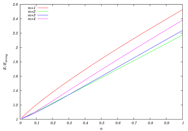
Figure 1: Comparison of the energy in the full and the strongly coupled (BPS) models as a function of the coupling constant $\alpha$, for Hopf charge $Q=m^{2}=1,4,9,16$. The fixed parameter values are $R_{0}=5$, $\beta=0.25$ and $\lambda=1$.

In a next step, we compare the corresponding energy densities. Here, we find a different behaviour for $m=1$, on the one hand, and for $|m|>1$, on the other hand. In Figure 2, we compare the (numerical) energy densities for $m=1$ for different values of $\alpha$ with the (analytical) energy density for $\alpha=0$ (strongly coupled model). We find that the energy density for small $\alpha$ uniformly approaches the $\alpha=0$ curve in the whole interval $z\in[0,1]$.

Figure 2: Energy densities in the full model, for different values of $\alpha$, and in the strongly coupled (BPS) model ($\alpha=0$) for Hopf charge $Q=m^{2}=1$, as a function of $z$. The fixed parameter values are $R_{0}=5$, $\beta=0.25$ and $\lambda=1$.

In Figures 3 - 5, we compare the (numerical) energy densities for $m=2,3,4$ for different values of $\alpha$ with the (analytical) energy density for $\alpha=0$ (strongly coupled model). In this case, we find that the curves for small but nonzero $\alpha$ approach the curve for $\alpha=0$ almost everywhere. There remains, however, a difference near $z=0$, where the curves for non-zero $\alpha$ approach a different value than the energy density for $\alpha=0$. The value at $z=0$ for non-zero $\alpha$ is, in fact, just one-half of the value for the case $\alpha=0$, as follows easily from the following argument. At $z=0$, for $\alpha>0$ only the potential term contributes to the energy density, whereas the gradient terms give no contribution. For $\alpha=0$, instead, the potential and the quartic gradient term give exactly the same contribution, as an immediate consequence of the Bogomolny nature of this solution. In the limit $\alpha\to 0$, this difference, however, is of measure zero and does not influence the value of the energy, as follows already from Figure (1).

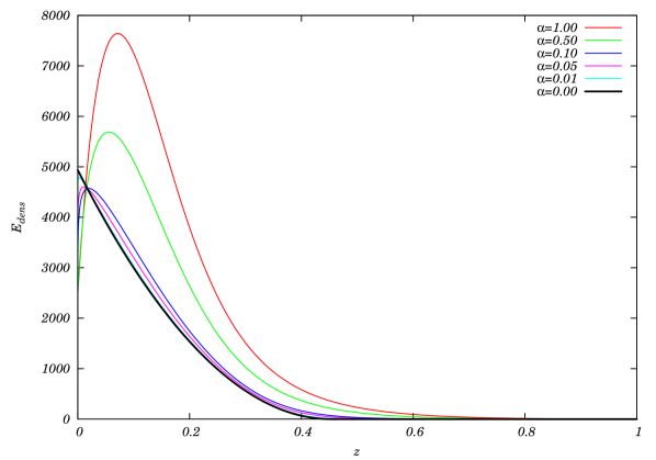
Figure 3: Energy densities in the full model, for different values of $\alpha$, and in the strongly coupled (BPS) model ($\alpha=0$) for Hopf charge $Q=m^{2}=4$, as a function of $z$. The fixed parameter values are $R_{0}=5$, $\beta=0.25$ and $\lambda=1$.

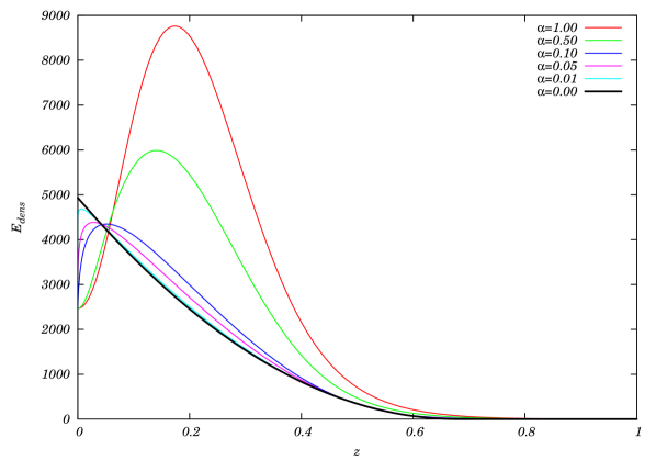
Figure 4: Energy densities in the full model, for different values of $\alpha$, and in the strongly coupled (BPS) model ($\alpha=0$) for Hopf charge $Q=m^{2}=9$, as a function of $z$. The fixed parameter values are $R_{0}=5$, $\beta=0.25$ and $\lambda=1$.

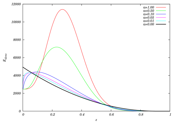
Figure 5: Energy densities in the full model, for different values of $\alpha$, and in the strongly coupled (BPS) model ($\alpha=0$) for Hopf charge $Q=m^{2}=16$, as a function of $z$. The fixed parameter values are $R_{0}=5$, $\beta=0.25$ and $\lambda=1$.

We remark that these findings are in complete agreement with the general discussion at the end of Section 3.

In Figures 6 - 9 we show the corresponding profile functions $g=1-(1/1+f^{2})$, for $m=1,2,3,4$. Again we find that the curves for small $\alpha$ approach the curve for $\alpha=0$ uniformly in the case of $m=1$, whereas there remains a small difference near $z=0$ for $|m|>1$. Indeed, for $\alpha=0$, $g$ behaves linear, i.e., like $g\sim 1-c_{1}z$ near $z=0$ for all $m$, whereas for $\alpha>0$ $g$ behaves like $g\sim 1-c_{m}\,z^{m}$.

Figure 6: Profile function $g$ in the full model, for different values of $\alpha$, and in the strongly coupled (BPS) model ($\alpha=0$) for Hopf charge $Q=m^{2}=1$, as a function of $z$. The fixed parameter values are $R_{0}=5$, $\beta=0.25$ and $\lambda=1$. At $z=0$, the behaviour is linear for all values of $\alpha$.

Figure 7: Profile function $g$ in the full model, for different values of $\alpha$, and in the strongly coupled (BPS) model ($\alpha=0$) for Hopf charge $Q=m^{2}=4$, as a function of $z$. The fixed parameter values are $R_{0}=5$, $\beta=0.25$ and $\lambda=1$. At $z=0$, the behaviour is linear for $\alpha=0$ and quadratic for $\alpha>0$.

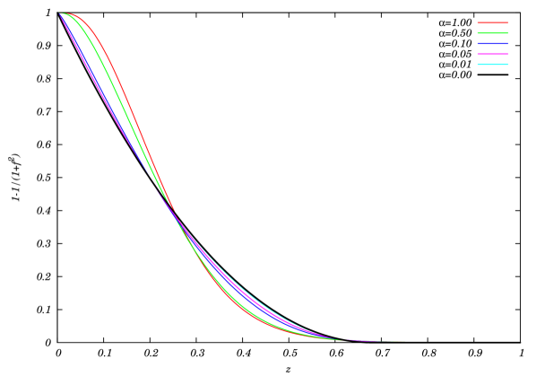
Figure 8: Profile function $g$ in the full model, for different values of $\alpha$, and in the strongly coupled (BPS) model ($\alpha=0$) for Hopf charge $Q=m^{2}=9$ , as a function of $z$. The fixed parameter values are $R_{0}=5$, $\beta=0.25$ and $\lambda=1$. At $z=0$, the behaviour is linear for $\alpha=0$ and cubic for $\alpha>0$.

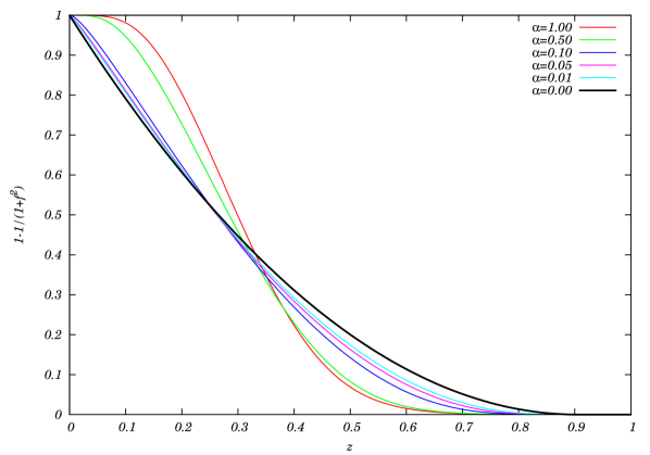
Figure 9: Profile function $g$ in the full model, for different values of $\alpha$, and in the strongly coupled (BPS) model ($\alpha=0$) for Hopf charge $Q=m^{2}=16$ , as a function of $z$. The fixed parameter values are $R_{0}=5$, $\beta=0.25$ and $\lambda=1$. At $z=0$, the behaviour is linear for $\alpha=0$ and quartic for $\alpha>0$.

6 Conclusions

It has been the main purpose of the present paper to investigate by means of analytical methods soliton solutions of the strongly coupled Skyrme–Faddeev–Niemi model (with only a quartic kinetic term) with a potential. We explicitly constructed compact solutions, which are natural generalizations of the compact solutions of the purely quartic baby Skyrme model which have first been reported by Gisiger and Paranjape [25], and further investigated recently [33]. As we wanted to present exact analytical solutions, we chose the base space (spacetime) $\mathbb{S}^{3}\times\mathbb{R}$ for finite energy solutions, because Minkowski spacetime does not offer sufficient symmetries to reduce the field equations to ordinary differential equations. Only in the case of spinning string-like solutions with a finite energy per length unit along the string the symmetry reduction in Minkowski space is possible (Section 4). For the case of $\mathbb{S}^{3}\times\mathbb{R}$ spacetime, we found two rather different classes of finite energy soliton solutions, namely compactons (which cover only a finite fraction of the three-sphere) on the one hand, and non-compact solitons (which cover the full three-sphere) on the other hand. Both classes of solutions are topological, but their energies are quite different. The compacton energies behave like $E_{c}\sim R_{0}|Q|^{1/2}$ (where $R_{0}$ is the radius of the three-sphere, and $Q$ is the topological charge), whereas the energies of the non-compact solitons behave like $E_{s}\sim R_{0}^{3}|Q|$. Further, the compactons only exist up to a certain maximum value of the topological charge, whereas the non-compact solitons start to exist from this value onwards. The different behaviors of the energies in the compact and non-compact case may be easily understood from the observation that the compactons obey a Bogomolny equation, whereas the non-compact solitons obey a “Bogomolny equation up to a constant”. Indeed, if for an energy density of the type ${\cal E}={\cal E}_{4}+{\cal E}_{0}$ (here the subindices refer to the power of first derivatives in each term) a Bogomolny equation holds, then the energy density for solutions may be expressed like ${\cal E}\sim({\cal E}_{4}{\cal E}_{0})^{1/2}$. If we now take into account the scaling dimensions ${\cal E}_{4}\sim R_{0}^{-4}$, ${\cal E}_{0}\sim R_{0}^{0}$ and $\int d^{3}x\sim R_{0}^{3}$, then the behaviour $E_{c}\sim R_{0}$ easily follows. Physically this means that the compacton solutions are localised near the north pole of the three-sphere, and the localisation becomes more pronounced for larger radii $R_{0}$. On the other hand, the energy density of the non-compact solitons remains essentially delocalised and evenly distributed over the whole three-sphere. We remark that the behavior of the compacton energies $E_{c}\sim R_{0}|Q|^{1/2}$ poses an apparent paradox, because it can be proven that already the quartic part of the energy alone can be bound from below by $|Q|$, that is, $E_{4}\equiv\int d^{3}x{\cal E}_{4}\geq\alpha R_{0}^{-1}|Q|$, where $\alpha$ is an unspecified constant. The proof was given in [35] for $R_{0}=1$, but the generalization for arbitrary radius is trivial using the scaling behavior of the corresponding terms. The apparent paradox is of course resolved by the observation that compactons exist only for not too large values of $|Q|$, such that the lower bound is compatible with the energies of the explicit solutions. Finally, if the potential has more than one vacuum, then compactons of the shell type exist, such that the field takes two different vacuum values inside the inner and outside the outer compact shell boundary. Except for their different shape, these compact shells behave quite similarly to the compact balls in the one-vacuum case (e.g. the relation between energy and topological charge or the linear growth of the energy with the three-sphere radius is the same).
Further, we found that the strongly coupled model reproduces the properties of the full model rather faithfully, at least on $\mathbb{S}^{3}$. Not only global properties like the topological charge and the energy, but also issues like the localized character (e.g., near the north pole) of a soliton are common properties of solutions of the strongly coupled and the full model, as we demonstrated in the numerical investigation in Section 5. We also found, however, that there exist some subtle, local differences for solutions with a topological charge $|Q|>1$.
To summarize, the inclusion of the potential term influences rather significantly qualitative as well as quantitative features of solitonic solutions: it modifies the energy-charge relation (especially for small values of the topological charge) and it leads to ball or shell-type solitons for one or two vacua potentials respectively.
One interesting question clearly is whether analogous properties (e.g.t the existence of compacton solutions with finite energy) can be observed in Minskowski space. An exact calculation is probably not possible in this case, but we think that we have found already some indirect evidence for the existence of such solutions. The first argument is, of course, the fact that they exist in one dimension lower (in the baby Skyrme model). The second argument is related to the behaviour of our solutions for large radius $R_{0}$. The compacton solutions are localized and, therefore, their energies grow only moderately with $R_{0}$ (linearly in $R_{0}$). Further, the allowed range of topological charges for compactons grows like the fourth power of $R_{0}$. These are clear indications that compacton solutions might also exist in Minkowski space. Certainly this question requires some further investigation. If these compactons in Minkowski space exist, then an interesting question is which energy-charge relation will result. Will the energies grow like $E_{c}\sim|Q|^{1/2}$, like on the three-sphere, or will they obey the three-quarter law $E_{c}\sim|Q|^{3/4}$, like for the full SFN model without potential in Minkowski space? All we can say at the moment is that an upper bound for the energy in flat space can be derived. The derivation is completely analogous to the cases of the full SFN, Nicole or AFZ models (the choice of trial functions which explicitly saturate the bound), and also the result is the same, $E_{c}\leq\alpha|Q|^{3/4}$, see [12]. The attempt to derive a lower bound, analogous to the Vakulenku-Kapitanski bound for the SFN model, meets the same obstacles as for the Nicole or AFZ models, see Appendix C of the second reference in [12].
Assuming for the moment the existence of compactons in Minkowski space, another interesting proposal is to use the compacton solutions of the pure quartic model (with potential) as a lowest order approximation to soliton solutions of the full SFN model and try to approximate the full solitons by a kind of generalized expansion. If such an approximate solution is possible, it would have several advantages.
$\bullet$ The pure quartic model is much easier than the full theory. In the case of the baby Skyrme model (both with old and new potentials) one gets even solvable models (as long as the rotational symmetry is assumed).
$\bullet$ The lowest order solution is already a non-perturbative configuration, i.e., a compacton, which captures the topological properties of the full solution. Due to the compact nature of the lowest order solution we have a kind of "localization" of the topological properties in a finite volume.
$\bullet$ One can easily construct multi-compacton solutions which, if sufficiently separated, do not interact. They form something which perhaps may be called a fake Bogomolny sector as they are solutions of a first order equation (usually saturating a corresponding energy-charge inequality) and may form multi-soliton noninteracting complexes.
Of course, it remains to be seen whether such an approximate solution is possible at all. What can be said so far is that in the simpler case of a scalar field theory with a potential which is smooth if a certain parameter $\mu$ is non-zero and approaches a V-shaped potential in the $\mu\to 0$ limit, then the compacton is the $\mu\to 0$ limit of the non-compact soliton, see [36]. Similarly, as was shown in the last section, the Hopf compactons of the strongly coupled model approximate the solitons of the full SFN theory, at least on $\mathbb{S}^{3}$ space.

References

- [1] L. Faddeev and A. J. Niemi, Nature 387, 58 (1997); Faddeev L and Niemi A 1999 Phys. Rev. Lett. 82 1624; L. Faddeev and A. J. Niemi, Nucl. Phys. B 776 (2007) 38
- [2] Y. M. Cho, Phys.Rev.D 21, 1080 (1980); Phys.Rev. D 23, 2415 (1981).
- [3] E. Radu, M.S. Volkov, Phys. Rept. 468 (2008) 101.
- [4] E. Babaev, L. Faddeev, A. Niemi, Phys. Rev. B 65, 100512 (2002); E. Babaev, Phys. Rev. Lett. 88, 177002 (2002)
- [5] J. Jaykka, J. Hietarinta, P. Salo, Phys. Rev. B77 (2008) 094509; J. Jaykka, Phys. Rev. D79 (2009) 065006
- [6] L. Faddeev, A. J. Niemi, U. Wiedner, Phys. Rev. D 70 (2004) 114033
- [7] L. Faddeev, A. J. Niemi, Phys. Lett. B 525, 195 (2002)
- [8] L. Dittmann, T. Heinzl and A. Wipf, Nucl. Phys. B (proc. Suppl.) 106 (2002) 649; L. Dittmann, T. Heinzl and A. Wipf, Nucl. Phys. B (proc. Suppl.) 108 (2002) 63.
- [9] Gladikowski J and Hellmund M 1997 Phys. Rev. D 56 5194
- [10] Battye R A and Sutcliffe P M 1998 Phys. Rev. Lett. 81 4798; Battye R A and Sutcliffe P M 1999 Proc.Roy.Soc.Lond. A 455 4305; Hietarinta J and Salo P 1999 Phys. Lett. B 451 60; Hietarinta J and Salo P 2000 Phys. Rev. D 62 81701; Sutcliffe P M 2007 arXiv:0705.1468; J. Jaykka, J. Hietarinta, Phys. Rev. D79 (2009)125027; J. Hietarinta, J. Jaykka, P. Salo, Phys. Lett. A321 (2004) 324.
- [11] A. F. Vakulenko, L. V. Kapitansky, Sov. Phys. Dokl, 24 (1979) 432
- [12] F. Lin and Y. Yang, Comm. Math. Phys. 249 (2004) 273; C. Adam, J. Sánchez-Guillén, R. A. Vazquez, A. Wereszczyński, J. Math. Phys. 47 (2006) 052302; M. Hirayama, H. Yamakoshi, J. Yamashita, Prog. Theor. Phys. 116 (2006) 273
- [13] R.S. Ward, Nonlinearity, 12 (1999) 241
- [14] R.S. Ward, Phys. Lett. B473 (2000) 291
- [15] Alvarez O, Ferreira L A and Sánchez-Guillén J 1998 Nucl. Phys. B 529 689
- [16] Hirayama M and Shi C-G 2007 Phys. Lett. B 652 384; C. Adam, J. Sánchez-Guillén, A. Wereszczyński, Phys. Lett. B661 (2008) 378; C. Adam, J. Sánchez-Guillén, A. Wereszczyński, Phys. Lett. B659 (2008) 761
- [17] L.A. Ferreira, arXiv:0809.4303
- [18] M. Hirayama, C.-G. Shi, J. Yamashita (2003) Phys. Rev. D 67:105009; M. Hirayama, C.-G. Shi (2004) Phys. Rev. D 69:045001
- [19] E. De Carli, L.A. Ferreira, J. Math. Phys. 46 (2005) 012703; C. Adam, J. Sánchez-Guillén, A. Wereszczyński, Eur. Phys. J. C47 (2006) 513; A.C. Riserio do Bonfim, L.A. Ferreira, JHEP 0603:097,2006; L.A. Ferreira, JHEP 0603:075,2006
- [20] Karliner M and Hen I, 2008 Nonlinearity 21 399; Karliner M and Hen I 2009 arXiv:0901.1489
- [21] B. M. A. G. Piette, B. J. Schoers and W J Zakrzewski, Z. Phys. C65 (1995) 165; B. M. A. G. Piette, B. J. Schoers and W J Zakrzewski, Nucl. Phys. B439 (1995) 205; R. A. Leese, M. Peyrard and W. J. Zakrzewski Nonlinearity 3 (1990) 773; B. M. A. G. Piete and W. J. Zakrzewski, Chaos, Solitons and Fractals 5 (1995) 2495; P. M. Sutcliffe, Nonlinearity (1991) 4 1109
- [22] T. Weidig, Nonlinearity 12 (1999) 1489
- [23] R. A. Battye, P. M. Sutcliffe, Nucl. Phys. B705 (2005) 384; R. A. Battye, P. M. Sutcliffe, Phys. Rev. C73 (2006) 055205; R. A. Battye, P. M. Sutcliffe, Phys. Rev. C80 (2009) 034323
- [24] J. M. Speight and M. Svensson, Commun. Math. Phys. 272 (2007) 751; R. Slobodeanu, arXiv:0812.4545
- [25] T. Gisiger and M. B. Paranjape, Phys. Rev. D 55 (1997) 7731
- [26] C. Adam, T. Romanczukiewicz, J. Sanchez-Guillen, A. Wereszczynski, Phys. Rev. D81 (2010) 085007
- [27] P. Sutcliffe, arXiv:1003.0023
- [28] C. Adam, J. Sánchez-Guillén, A. Wereszczyński, arXiv:1001.4544
- [29] L. A. Ferreira, arXiv:0912.3404
- [30] H. Aratyn , L.A. Ferreira, A.H. Zimerman, Phys. Lett. B 456 (1999) 162.
- [31] C. Adam, J. Sanchez-Guillen, A. Wereszczynski, J. Math. Phys. 47, 022303 (2006).
- [32] H. Arodz, J. Lis, Phys. Rev. D77, 107702 (2008); H. Arodz, J. Karkowski, Z. Swierczynski, arXiv:0907.2801
- [33] C. Adam, P. Klimas, J. Sánchez-Guillén, A. Wereszczyński, Phys. Rev. D80, 105013 (2009)
- [34] P. Rosenau, J. H. Hyman, Phys. Rev. Lett. 70 (1993) 564; Arodź H 2002 Acta Phys. Polon. B 33 1241; Arodź H 2004 Acta Phys. Polon. B 35 625
- [35] J. M. Speight, M. Svensson, arXiv:0804.4385
- [36] J. Lis, arXiv:0911.3423