Ejectile Polarization for ${}^{2}H(e,e^{\prime}\vec{p})n$ at GeV energies

Abstract

We perform a fully relativistic calculation of the ${}^{2}H(e,e^{\prime}\vec{p})n$ reaction in the impulse approximation employing the Gross equation to describe the deuteron ground state, and we use the SAID parametrization of the full NN scattering amplitude to describe the final state interactions (FSIs). The formalism for treating the ejectile polarization with a spin projection on an arbitrary axes is discussed. We show results for the six relevant asymmetries and discuss the role of spin-dependent FSI contributions.

I Introduction

Exclusive electron scattering from the deuteron target is very interesting by itself, and it also is a very relevant stepping stone towards understanding exclusive electron scattering from heavier nuclei. The $D(e,e^{\prime}p)n$ reaction at GeV energies allows us - and requires us - to carefully study the reaction mechanism. It is necessary to consider final state interactions (FSIs) between the two nucleons in the final state, two-body currents, and isobar contributions. Of these, the FSIs can be expected to be the most relevant part of the reaction mechanisms at the GeV energy and momentum transfers relevant to the study of the transition from hadronic to quark-gluon degrees of freedom. For some recent reviews on this exciting topic, see e.g. wallyreview ; ronfranz ; sickreview .

The fact that the deuteron is the simplest nucleus enables us to study all facets of the reaction mechanism in great detail. Anything that can be gleaned from the deuteron will be highly useful for heavier nuclei. Exclusive electron scattering from nuclei is one type of reaction where one may observe color transparency cteep , and the deuteron itself provides a laboratory for the study of neutrons, e.g. the neutron magnetic form factor hallbgmn . The short range structures studied in exclusive electron scattering might even reveal information about the properties of neutron stars misakneutstar .

It is important to use all available tools to further our understanding of exclusive scattering from the deuteron. While unpolarized scattering is interesting, polarization observables hold the promise of revealing more detailed information about the reaction mechanism. It is therefore important and interesting to test one’s model for polarized observables, too.

In bigdpaper , we performed a fully relativistic calculation of the $D(e,e^{\prime}p)n$ reaction, using a relativistic wave function wallyfranzwf and $NN$ scattering data said for our calculation of the full, spin-dependent final state interactions (FSIs). The main difference to many other high quality calculations using the generalized eikonal approximation misak ; ciofi ; genteikonal ; misakbrandnew or a diagrammatic approach laget is the inclusion of all the spin-dependent pieces in the nucleon-nucleon amplitude. Full FSIs have recently been included in schiavilla . Several experiments with unpolarized deuterons are currently under analysis or have been published recently, egiyansrc ; halladata ; hallbgmn ; jerrygexp ; blast . There are also new proposals for D(e,e’p) experiments at Jefferson Lab wernernewprop .

In bigdpaper , we focused on observables that are accessible for an unpolarized target and an unpolarized nucleon detected in the final state. The spin-dependent pieces in our FSI calculation were particularly relevant for the fifth response function, an observable that can be measured only with polarized electron beams. The spin-dependent contributions also contributed significantly to the strength in the FSI-dominated regions of the unpolarized cross section. Naturally, experiments with polarization of the target or ejectile are harder to perform than their unpolarized counterparts. However, the extra effort allows one to study otherwise inaccessible observables that are rather sensitive to certain properties of the nuclear ground state and the reaction mechanism. Recently, we investigated the target polarization in $\vec{D}(e,e^{\prime}p)n$ and $\vec{D}(\vec{e},e^{\prime}p)n$ targetpol . In this paper, we study the asymmetries accessible with a polarized ejectile proton, and a polarized or unpolarized electron beam. As before, the focus of our numerical calculations is the kinematic region accessible at GeV energies, i.e. the kinematic range of Jefferson Lab.

Recoil polarization measurement have often been performed for $(e,e^{\prime}\vec{n})$ reactions, to measure the neutron electric form factor via polarization transfer. These measurements typically take place at rather low missing momentum. We can perform $D(e,e^{\prime}\vec{n})$ calculations just as easily as $D(e,e^{\prime}\vec{p})$ calculations. For simplicity, we focus on ejectile proton polarization in our numerical results.

A measurement of two recoil proton polarizations for low missing momentum and various $Q^{2}$, up to $1.6$ GeV², was performed at Jefferson Lab hudata . This was an interesting experiment that used the deuteron as a proton target, and checked if the deuteron is a good proton target - this is relevant for using the deuteron as a neutron target. At much lower $Q^{2}$, there are data from Mainz mainzrecoil and Bates batesdeuteronrecoil for hydrogen and deuteron targets. Recoil polarimetry has been used more often for hydrogen targets than deuteron targets, also at Jefferson Lab protonelasticrecoil_highqsq ; protonelasticrecoil_lowqsq . Recoil polarimetry continues to be an interesting experimental technique fpp_technical , and it has been used also for heavier nuclei batescarbonrecoil , for photodisintegration photodisrecoil and in pion production kellypionprod .

This paper is organized as follows: in the next section, we introduce the necessary formalism to define the relevant observables. In particular, we discuss how to define reduced responses with explicit dependence on the azimuthal angle of the proton, and we discuss the projection of the proton spin on the most suitable coordinate system. We define six relevant asymmetries. Then, we present our numerical results, in a kinematic region relevant to experiments at Jefferson Lab. We show momentum distributions of all six asymmetries, and we discuss the contributions of the various spin-dependent parts of the final state interactions. We conclude with a brief summary.

II Formalism

II.1 Differential Cross Section

The standard coordinate systems used to describe the $D(e,e^{\prime}p)$ reaction are shown in Fig.1. The initial and final electron momenta $\bm{k}$ and $\bm{k^{\prime}}$ define the electron scattering plane and the $xyz$-coordinate system is defined such that the $z$ axis, the quantization axis, lies along the momentum of the virtual photon $q$ with the $x$-axis in the electron scattering plane and the $y$-axis perpendicular to the plane. The momentum $p$ of the outgoing proton is in general not in this plane and is located relative to the $xyz$ system by the polar angle $\theta_{p}$ and the azimuthal angle $\phi_{p}$. A second coordinate system $x^{\prime}y^{\prime}z^{\prime}$, is chosen such that the $z^{\prime}$-axis is parallel to the $z$-axis and the $x^{\prime}$-axis lies in the hadron plane formed by $\bm{p}$ and $\bm{q}$ and the $y^{\prime}$-axis is normal to this plane. The unit vectors in the primed system are defined in terms of the unprimed system as

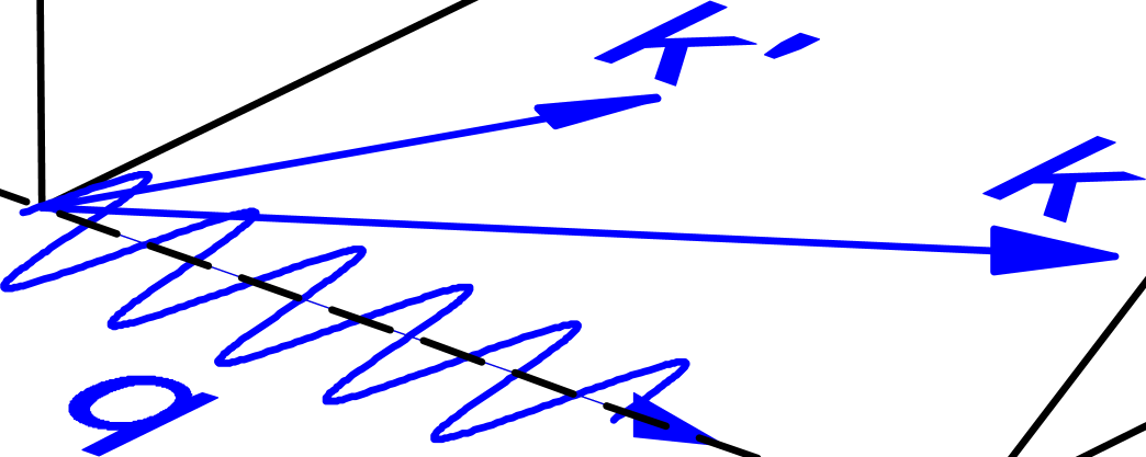
Figure 1: (Color online) Coordinate systems for the $D(e,e^{\prime}p)$ reaction. $k$ and $k^{\prime}$ are the initial and final electron four-momenta, $q$ is the four-momentum of the virtual photon and $p$ is the four-momentum of the final-state proton.

$$\hat{x}^{\prime} = \cos\phi_{p}\,\hat{x}+\sin\phi_{p}\,\hat{y}$$

$$\hat{y}^{\prime} = -\sin\phi_{p}\,\hat{x}+\cos\phi_{p}\,\hat{y}$$

$$\hat{z}^{\prime} = \hat{z}\,.$$ (1)

The general form of the $D(e,e^{\prime}p)$ cross section can be written in the lab frame as raskintwd ; dmtrgross

$$\left(\frac{d\sigma^{5}}{d\epsilon^{\prime}d\Omega_{e}d\Omega_{p}}\right)_{h} = \frac{m_{p}\,m_{n}\,p_{p}}{16\pi^{3}\,M_{d}}\,\sigma_{Mott}\,f_{rec}^{-1}\,\Big{[}v_{L}R_{L}+v_{T}R_{T}+v_{TT}R_{TT}+v_{LT}R_{LT}$$ (2)

$$+h\,v_{LT^{\prime}}R_{LT^{\prime}}+h\,v_{T^{\prime}}R_{T^{\prime}}\Big{]}\,,$$

where $M_{d}$, $m_{p}$ and $m_{n}$ are the masses of the deuteron, proton and neutron, $p_{p}=p_{1}$ and $\Omega_{p}$ are the momentum and solid angle of the ejected proton, $\epsilon^{\prime}$ is the energy of the detected electron and $\Omega_{e}$ is its solid angle, with $h=\pm 1$ for positive and negative electron helicity. The Mott cross section is

$$\sigma_{Mott}=\left(\frac{\alpha\cos(\theta_{e}/2)}{2\varepsilon\sin^{2}(\theta_{e}/2)}\right)^{2}$$ (3)

and the recoil factor is given by

$$f_{rec}=\left|1+\frac{\omega p_{p}-E_{p}q\cos\theta_{p}}{M_{d}\,p_{p}}\right|\,.$$ (4)

The leptonic coefficients $v_{K}$ are

$$v_{L} = \frac{Q^{4}}{q^{4}}$$ (5)

$$v_{T} = \frac{Q^{2}}{2q^{2}}+\tan^{2}\frac{\theta_{e}}{2}$$ (6)

$$v_{TT} = -\frac{Q^{2}}{2q^{2}}$$ (7)

$$v_{LT} = -\frac{Q^{2}}{\sqrt{2}q^{2}}\sqrt{\frac{Q^{2}}{q^{2}}+\tan^{2}\frac{\theta_{e}}{2}}$$ (8)

$$v_{LT^{\prime}} = -\frac{Q^{2}}{\sqrt{2}q^{2}}\tan\frac{\theta_{e}}{2}$$ (9)

$$v_{T^{\prime}} = \tan\frac{\theta_{e}}{2}\sqrt{\frac{Q^{2}}{q^{2}}+\tan^{2}\frac{\theta_{e}}{2}}$$ (10)

Within this general framework, we have two options for evaluating the response functions: first, we will give expressions for the response functions in terms of matrix elements that are defined with respect to the electron plane, i.e. the $xyz$ plane. These matrix elements are implicitly dependent on $\phi_{p}$, the angle between hadron plane and electron plane, and these are the responses used e.g. in raskintwd . Second, we give expressions for the responses in the $x^{\prime}y^{\prime}z^{\prime}$ plane. All quantities given relative to the $x^{\prime}y^{\prime}z^{\prime}$ coordinate system are denoted by a line over the quantity. The current matrix elements, and therefore the response functions, in the $x^{\prime}y^{\prime}z^{\prime}$ coordinate system do not have any $\phi_{p}$ dependence. It is much more practical to evaluate the responses in the $x^{\prime}y^{\prime}z^{\prime}$ coordinate system. The commonly used responses in the $xyz$ system can then easily be obtained by accounting for the $\phi_{p}$ dependence explicitly, see eq.(17) below, instead of newly evaluating matrix elements for each value of $\phi_{p}$. Note that both coordinate systems use the same quantization axis: the $z$ axis and the $z^{\prime}$ axis are parallel.

The hadronic tensor for production of polarized protons is defined as

$$w_{\lambda^{\prime}_{\gamma},\lambda_{\gamma}}(\hat{{\cal S}})=\frac{2}{3}\sum_{s_{1},s^{\prime}_{1},s_{2},\lambda_{d}}\left<\bm{p}_{1}s^{\prime}_{1};\bm{p}_{2}s_{2};(-)\right|J_{\lambda^{\prime}_{\gamma}}\left|\bm{P}\lambda_{d}\right>^{*}\left<\bm{p}_{1}s_{1};\bm{p}_{2}s_{2};(-)\right|J_{\lambda_{\gamma}}\left|\bm{P}\lambda_{d}\right>{\cal P}_{s^{\prime}_{1}s_{1}}(\hat{{\cal S}})$$ (11)

where

$$J_{\pm 1}=\mp\frac{1}{\sqrt{2}}(J^{1}\pm J^{2})$$ (12)

and

$$J_{0}=J^{0}$$ (13)

is the charge operator. The notation $(-)$ in the final state indicates that the state satisfies the boundary conditions appropriate for an “out” state. The operator

$$\bm{{\cal P}}(\hat{{\cal S}})=\frac{1}{2}\left(\bm{1}+\bm{\sigma}\cdot\hat{{\cal S}}\right)$$ (14)

is a spin projection operator that projects the proton spin onto unit vector $\hat{{\cal S}}$ which corresponds to the direction of the proton spin in its rest frame relative to the $xyz$-system.

The response functions in the $xyz$-frame are given by

$$R_{L}(\hat{{\cal S}}) = w_{00}(\hat{{\cal S}})$$

$$R_{T}(\hat{{\cal S}}) = w_{11}(\hat{{\cal S}})+w_{-1-1}(\hat{{\cal S}})$$

$$R_{TT}(\hat{{\cal S}}) = 2\mbox{Re}(w_{1-1}(\hat{{\cal S}}))$$

$$R_{LT}(\hat{{\cal S}}) = -2\mbox{Re}(w_{01}(\hat{{\cal S}})-w_{0-1}(\hat{{\cal S}}))$$

$$R_{LT^{\prime}}(\hat{{\cal S}}) = -2\mbox{Re}(w_{01}(\hat{{\cal S}})+w_{0-1}(\hat{{\cal S}}))$$

$$R_{T^{\prime}}(\hat{{\cal S}}) = w_{11}(\hat{{\cal S}})-w_{-1-1}(\hat{{\cal S}})\,.$$ (15)

Now we proceed to write down expressions for the responses in the $x^{\prime}y^{\prime}z^{\prime}$ coordinate system. Calculating the responses in this system offers a faster alternative to the above calculation, which requires a new evaluation of the current matrix elements for each $\phi_{p}$ value. The response functions defined above are implicitly dependent upon the angle $\phi_{p}$ between the electron plane and the hadron plane containing the proton and neutron in the final state. This dependence can be made explicit by noting that

$$\left<\bm{p}_{1}s_{1};\bm{p}_{2}s_{2};(-)\right|J_{\lambda_{\gamma}}\left|\bm{P}\lambda_{d}\right>=e^{i(\lambda_{d}+\lambda_{\gamma}-s_{1}-s_{2})\phi_{p}}\overline{\left<\bm{p}_{1}s_{1};\bm{p}_{2}s_{2};(-)\right|J_{\lambda_{\gamma}}\left|\bm{P}\lambda_{d}\right>}$$ (16)

where the line over the matrix elements is used to indicate that they are quantized relative to the $x^{\prime}y^{\prime}z^{\prime}$ coordinate system. The hadronic tensor can then be written as

$$w_{\lambda^{\prime}_{\gamma},\lambda_{\gamma}}(\hat{{\cal S}})=e^{-i(\lambda^{\prime}_{\gamma}-\lambda_{\gamma})\phi_{p}}\overline{w}_{\lambda^{\prime}_{\gamma},\lambda_{\gamma}}(\overline{\hat{{\cal S}}})$$ (17)

where

$$\overline{w}_{\lambda^{\prime}_{\gamma},\lambda_{\gamma}}(\overline{\hat{{\cal S}}})=\frac{2}{3}\sum_{s_{1},s^{\prime}_{1}s_{2},\lambda_{d}}\overline{\left<\bm{p}_{1}s^{\prime}_{1};\bm{p}_{2}s_{2};(-)\right|J_{\lambda^{\prime}_{\gamma}}\left|\bm{P}\lambda^{\prime}_{d}\right>}^{*}\overline{\left<\bm{p}_{1}s_{1};\bm{p}_{2}s_{2};(-)\right|J_{\lambda_{\gamma}}\left|\bm{P}\lambda_{d}\right>}{\cal P}_{s^{\prime}_{1}s_{1}}(\overline{\hat{{\cal S}}})$$ (18)

and

$${\cal P}_{s^{\prime}_{1}s_{1}}(\hat{\overline{{\cal S}}})=e^{i(s^{\prime}_{1}-s_{1})\phi_{p}}{\cal P}_{s^{\prime}_{1}s_{1}}(\hat{{\cal S}})=\frac{1}{2}\left(\bm{1}+\bm{\sigma}\cdot\hat{\overline{{\cal S}}}\right)_{s^{\prime}_{1}s_{1}}$$ (19)

is the spin projection operator defined relative to the $x^{\prime}y^{\prime}z^{\prime}$ coordinate system. Note that this can be obtained by simply decomposing the unit vector $\hat{{\cal S}}$ in terms of the $x^{\prime}y^{\prime}z^{\prime}$ basis.

Using eq. (17) and the definition of the responses in the $xyz$ system, eq. (15), the response functions in the $x^{\prime}y^{\prime}z^{\prime}$ system then become

$$R_{L}(\hat{\overline{{\cal S}}}) = \overline{R}_{L}^{(I)}(\hat{\overline{{\cal S}}})$$

$$R_{T}(\hat{\overline{{\cal S}}}) = \overline{R}_{T}^{(I)}(\hat{\overline{{\cal S}}})$$

$$R_{TT}(\hat{\overline{{\cal S}}}) = \overline{R}_{TT}^{(I)}(\hat{\overline{{\cal S}}})\cos 2\phi_{p}+\overline{R}_{TT}^{(II)}(\hat{\overline{{\cal S}}})\sin 2\phi_{p}$$

$$R_{LT}(\hat{\overline{{\cal S}}}) = \overline{R}_{LT}^{(I)}(\hat{\overline{{\cal S}}})\cos\phi_{p}+\overline{R}_{LT}^{(II)}(\hat{\overline{{\cal S}}})\sin\phi_{p}$$

$$R_{LT^{\prime}}(\hat{\overline{{\cal S}}}) = \overline{R}_{LT^{\prime}}^{(I)}(\hat{\overline{{\cal S}}})\sin\phi_{p}+\overline{R}_{LT^{\prime}}^{(II)}(\hat{\overline{{\cal S}}})\cos\phi_{p}$$

$$R_{T^{\prime}}(\hat{\overline{{\cal S}}}) = \overline{R}_{T^{\prime}}^{(II)}(\hat{\overline{{\cal S}}})$$ (20)

where the reduced response functions for the two classes I and II are defined in terms of the hadronic tensors as

$$\overline{R}^{(I)}_{L}(\hat{\overline{{\cal S}}}) = \overline{w}_{00}(\hat{\overline{{\cal S}}})$$

$$\overline{R}^{(I)}_{T}(\hat{\overline{{\cal S}}}) = \overline{w}_{1,1}(\hat{\overline{{\cal S}}})+\overline{w}_{-1,-1}(\hat{\overline{{\cal S}}})$$

$$\overline{R}^{(I)}_{TT}(\hat{\overline{{\cal S}}}) = 2\mbox{Re}(\overline{w}_{1,-1}(\hat{\overline{{\cal S}}}))$$

$$\overline{R}^{(II)}_{TT}(\hat{\overline{{\cal S}}}) = 2\mbox{Im}(\overline{w}_{1,-1}(\hat{\overline{{\cal S}}}))$$

$$\overline{R}^{(I)}_{LT}(\hat{\overline{{\cal S}}}) = -2\mbox{Re}(\overline{w}_{01}(\hat{\overline{{\cal S}}})-\overline{w}_{0-1}(\hat{\overline{{\cal S}}}))$$

$$\overline{R}^{(II)}_{LT}(\hat{\overline{{\cal S}}}) = 2\mbox{Im}(\overline{w}_{01}(\hat{\overline{{\cal S}}})+\overline{w}_{0-1}(\hat{\overline{{\cal S}}}))$$

$$\overline{R}^{(I)}_{LT^{\prime}}(\hat{\overline{{\cal S}}}) = 2\mbox{Im}(\overline{w}_{01}(\hat{\overline{{\cal S}}})-\overline{w}_{0-1}(\hat{\overline{{\cal S}}}))$$

$$R^{(II)}_{LT^{\prime}}(\hat{\overline{{\cal S}}}) = -2\mbox{Re}(\overline{w}_{01}(\hat{\overline{{\cal S}}})+\overline{w}_{0-1}(\hat{\overline{{\cal S}}}))$$

$$\overline{R}^{(II)}_{T^{\prime}}(\hat{\overline{{\cal S}}}) = \overline{w}_{1,1}(\hat{\overline{{\cal S}}})-\overline{w}_{-1,-1}(\hat{\overline{{\cal S}}})\,.$$ (21)

The reduced response functions still retain some implicit $\phi$ dependence associated with the choice of the arbitrary direction of $\hat{{\cal S}}$ which is fixed relative to the $xyz$ system. This can be made explicit by defining a new set of unit vectors, usually referred to as normal, longitudinal, and sideways,

$$\hat{n} = \hat{y}^{\prime}$$ (22)

$$\hat{l} = \sin\theta_{p}\,\hat{x}^{\prime}+\cos\theta_{p}\,\hat{z}^{\prime}$$ (23)

$$\hat{s} = \cos\theta_{p}\,\hat{x}^{\prime}-\sin\theta_{p}\,\hat{z}^{\prime}$$ (24)

fixed relative to the $x^{\prime}y^{\prime}z^{\prime}$ system such that $\hat{l}$ lies along the proton direction with $\hat{s}$ is in the hadron plane and $\hat{n}$ is normal to it. We decompose the spin-dependent part of the projection operator as

$$\bm{\sigma}\cdot\hat{\overline{{\cal S}}}=\bm{\sigma}\cdot\hat{n}\ \hat{n}\cdot\hat{\overline{{\cal S}}}+\bm{\sigma}\cdot\hat{l}\ \hat{l}\cdot\hat{\overline{{\cal S}}}+\bm{\sigma}\cdot\hat{s}\ \hat{s}\cdot\hat{\overline{{\cal S}}}$$ (25)

The response functions can be further expanded as

$$\overline{R}^{(I)}_{K}(\hat{\overline{{\cal S}}})=\overline{R}_{K}(\bm{1})+\overline{R}_{K}(\bm{\sigma}\cdot\hat{n})\hat{n}\cdot\hat{\overline{{\cal S}}}$$ (26)

and

$$\overline{R}^{(II)}_{K}(\hat{\overline{{\cal S}}})=\overline{R}_{K}(\bm{\sigma}\cdot\hat{l})\hat{l}\cdot\hat{\overline{{\cal S}}}+\overline{R}_{K}(\bm{\sigma}\cdot\hat{s})\hat{s}\cdot\hat{\overline{{\cal S}}}$$ (27)

where the response functions $\overline{R}_{K}(\cal{O})$, ${\cal O}\in\left\{\bm{1},\bm{\sigma}\cdot\hat{n},\bm{\sigma}\cdot\hat{l},\bm{\sigma}\cdot\hat{s}\right\}$, can be obtained from (21) using the response tensors

$$\overline{w}_{\lambda^{\prime}_{\gamma},\lambda_{\gamma}}({\cal O})=\frac{1}{3}\sum_{s_{1},s^{\prime}_{1},s_{2},\lambda_{d}}\overline{\left<\bm{p}_{1}s^{\prime}_{1};\bm{p}_{2}s_{2};(-)\right|J_{\lambda^{\prime}_{\gamma}}\left|\bm{P}\lambda^{\prime}_{d}\right>}^{*}\overline{\left<\bm{p}_{1}s_{1};\bm{p}_{2}s_{2};(-)\right|J_{\lambda_{\gamma}}\left|\bm{P}\lambda_{d}\right>}{\cal O}_{s^{\prime}_{1}s_{1}}\,,$$ (28)

The new response functions are now independent of $\phi_{p}$ with any residual dependence on $\phi_{p}$ now contained in the inner products $\hat{n}\cdot\hat{\overline{{\cal S}}}$, $\hat{l}\cdot\hat{\overline{{\cal S}}}$ and $\hat{s}\cdot\hat{\overline{{\cal S}}}$.

It is often convenient to use a simplified notation for these new response functions where

$$\overline{R}_{K} = \overline{R}_{K}(\bm{1})$$

$$\overline{R}^{n}_{K} = \overline{R}_{K}(\bm{\sigma}\cdot\hat{n})$$

$$\overline{R}^{l}_{K} = \overline{R}_{K}(\bm{\sigma}\cdot\hat{l})$$

$$\overline{R}^{s}_{K} = \overline{R}_{K}(\bm{\sigma}\cdot\hat{s})\,,$$ (29)

and $\overline{R}_{K}$ corresponds to the unpolarized response.

Note that when $\theta_{p}$ is either $0$ or $\pi$, the hadron plane, and therefore the angle $\phi_{p}$, is no longer defined. As a result the cross section at these angles must be independent of the azimuthal angle $\phi_{p}$. This imposes constraints on the reduced response functions. The constraints can be obtained by writing the response functions $R_{K}(\hat{\overline{{\cal S}}})$ of (20) for arbitrary $\hat{{\cal S}}$ in terms of the $\overline{R}^{I}_{K}$ with the inner products given explicitly as functions of $\theta_{p}$ and $\phi_{p}$. Each of the $R_{K}(\hat{\overline{{\cal S}}})$ can be expanded to lowest order about $\theta_{p}=0(\pi)$. The result can then be written as a Fourier series in $\phi_{p}$. In order for the cross section to be independent of $\phi_{p}$ at forward and backward angles all of the coefficients of non-constant terms in the Fourier series must vanish in the limit $\theta_{p}\rightarrow 0(\pi)$. The resulting equations result in constraints on the $\overline{R}^{I}_{K}$. From this analysis, the response functions $\overline{R}_{L}$, $\overline{R}_{T}$, $\overline{R}^{n}_{LT}$, $\overline{R}^{n}_{LT^{\prime}}$ and $\overline{R}^{l}_{T^{\prime}}$ are unconstrained at these angles while $\overline{R}^{s}_{LT}=\pm\overline{R}^{n}_{LT}$ and $\overline{R}^{s}_{LT^{\prime}}=\mp\overline{R}^{n}_{LT^{\prime}}$ for $\theta_{p}=0,\pi$. All other response functions must vanish at forward and backward angles.

II.2 Asymmetries

The definition of asymmetries for polarized protons must be done carefully. Experiments to date have been done for the case where $\phi_{p}=0$. In this case the asymmetries have been determined relative to the unit vectors $\hat{n}$, $\hat{l}$ and $\hat{s}$. However, the use of this approach for out-of-plane measurements results in asymmetries that depend on $\phi_{p}$ when $\theta_{p}=0,\pi$. Therefore, our goal is to define a coordinate system that will be defined unambiguously even if $\theta_{p}=0,\pi$. It turns out that a reference frame suggested by the experimental set-up fulfills this requirement.

Another approach can be defined by noting that if a magnetic spectrometer is used to detect the proton, out-of-plane angles are most conveniently reached by tilting the spectrometer relative to the lab floor with the horizontal direction in the spectrometer remaining fixed. As a result, a new set of coordinates can be chosen such that the longitudinal axis lies along the direction of the proton and the sideways direction remains parallel to the electron scattering plane. The unit vectors defining this system are then given by

$$\hat{l}^{\prime} = \hat{l}$$ (30)

$$\hat{s}^{\prime} = \frac{\hat{y}\times\hat{l}}{|\hat{y}\times\hat{l}|}$$ (31)

$$\hat{n}^{\prime} = \hat{l}^{\prime}\times\hat{s}^{\prime}\,.$$ (32)

Choosing $\hat{\overline{{\cal S}}}=\hat{n}^{\prime}$, the unpolarized part of the cross section, which is independent of $\hat{n}^{\prime}$ can be written as

$$\sigma(0)+h\sigma_{h}(0)$$ (33)

and the part of the cross section proportional to $\hat{n}^{\prime}$ can be written as

$$\sigma(n^{\prime})+h\sigma_{h}(n^{\prime})$$ (34)

and choosing $\hat{\overline{{\cal S}}}=\hat{l}^{\prime}$ or $\hat{\overline{{\cal S}}}=\hat{s}^{\prime}$ can be used to obtain the contributions

$$\sigma(l^{\prime})+h\sigma_{h}(l^{\prime})$$ (35)

and

$$\sigma(s^{\prime})+h\sigma_{h}(s^{\prime})$$ (36)

The single and double asymmetries are now defined as

$$A^{\xi}_{p}=\frac{\sigma(\xi)}{\sigma(0)}$$ (37)

and

$$A^{\xi}_{ep}=\frac{\sigma_{h}(\xi)}{\sigma(0)}$$ (38)

where $\xi=n^{\prime},l^{\prime},s^{\prime}$. These asymmetries can be shown to be independent of $\phi_{p}$ for $\theta_{p}=0,\pi$.

II.3 Current Matrix Elements

A detailed description of the impulse approximation current matrix elements used here is presented in bigdpaper . These matrix elements are constructed based on the covariant spectator approximation grosseqn . A relativistic wave function wallyfranzwf and $NN$ scattering data said are used for our calculation of the full, spin-dependent final state interactions. The main difference to many other high quality calculations using the generalized eikonal approximation misak ; misakbrandnew ; ciofi ; genteikonal or a diagrammatic approach laget is the inclusion of all the spin-dependent pieces in the nucleon-nucleon amplitude. Full FSIs have recently been included in schiavilla .

To construct the scattering amplitudes needed for the calculation of the FSIs we start with $np$ helicity matrices extracted from SAID said . The on-shell scattering amplitudes can be given in terms of five Fermi invariants as

$$M_{ab;cd} = \mathcal{F}_{S}(s,t)\delta_{ac}\delta_{bd}+\mathcal{F}_{V}(s,t)\gamma_{ac}\cdot\gamma_{bd}+\mathcal{F}_{T}(s,t)\sigma^{\mu\nu}_{ac}(\sigma_{\mu\nu})_{bd}$$ (39)

$$+\mathcal{F}_{P}(s,t)\gamma^{5}_{ac}\gamma^{5}_{bd}+\mathcal{F}_{A}(s,t)(\gamma^{5}\gamma)_{ac}\cdot(\gamma^{5}\gamma)_{bd}$$

where $s$ and $t$ are the usual Mandelstam variables. The Fermi invariants are then determined using the helicity amplitudes. A table of the invariant functions is constructed in terms of $s$ and the center of momentum angle $\theta$. The table is then interpolated to obtain the invariant functions at the values required by the integration.

In order to estimate the possible effects of this contribution to the current matrix elements, we use a simple prescription for the off-shell behavior of the amplitude. Although additional invariants are possible when the nucleon is allowed to go off shell, we keep only the forms in (39). The center-of-momentum angle is calculated using

$${\cos\theta=\frac{t-u}{\sqrt{s-4m^{2}}\sqrt{\frac{(4m^{2}-t-u)^{2}}{s}-4m^{2}}}}$$ (40)

The invariants are then replaced by

$$\mathcal{F}_{i}(s,t)\rightarrow\mathcal{F}_{i}(s,t,u)F_{N}(s+t+u-3m^{2})$$ (41)

where

$$F_{N}(p^{2})=\frac{(\Lambda_{N}^{2}-m^{2})^{2}}{(p^{2}-m^{2})^{2}+(\Lambda_{N}^{2}-m^{2})^{2}}$$ (42)

and the $\mathcal{F}_{i}(s,t,u)$ are obtained from interpolation of the on-shell invariant functions with the center-of-momentum angle obtained from (40). The form factor (42) is used as a cutoff to limit contributions where the nucleon is highly off shell. We use a value of $\Lambda_{N}=1$ GeV in this paper. The numerical effects of variations in the cut-off parameter have been studied in bigdpaper .

III Results

III.1 Momentum Distributions

In order to give a general overview of the properties of all six asymmetries, we show them in Fig. 2 as three-dimensional plots versus the missing momentum and the azimuthal angle of the proton, $\phi_{p}$. From these plots, it becomes obvious that any statements about the relative size of the asymmetries are highly dependent on the independent variables, and none of the asymmetries can be singled out as “the largest” or “the smallest” in general. If one restricts one’s interest to in-plane measurements, i.e. to $\phi_{p}\approx 0^{o}$, one will observe that $A^{l^{\prime}}_{ep}$ is larger than the other observables, and $A^{n^{\prime}}_{p}$ and $A^{l^{\prime}}_{p}$ are medium-sized, but this is a $\phi_{p}$ dependent statement.

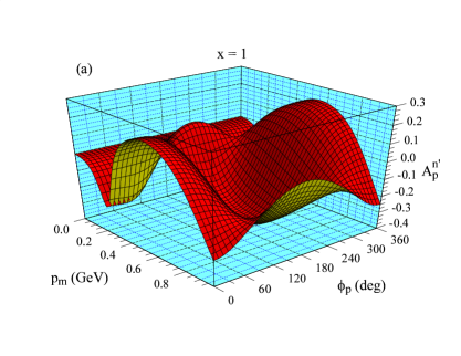
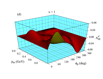
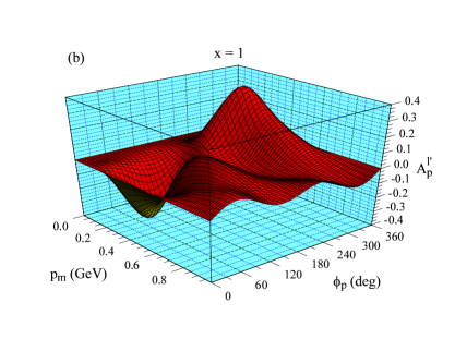
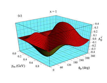
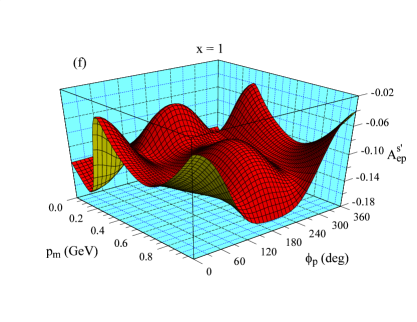
Figure 2: (Color online) The six panels show the six asymmetries plotted versus the missing momentum $p_{m}$ and versus the azimuthal angle of the proton, $\phi_{p}$, for a beam energy of $5.5$ GeV, a transferred four-momentum of $Q^{2}=2$ GeV², and $x=1$. We show $A^{n^{\prime}}_{p}$ (panel a)), $A^{l^{\prime}}_{p}$ (panel b)), $A^{s^{\prime}}_{p}$ (panel c)), $A^{n^{\prime}}_{ep}$ (panel d)), $A^{l^{\prime}}_{ep}$ (panel e)), and $A^{s^{\prime}}_{ep}$ (panel f)). The curves shown have been calculated including on-shell FSIs.

Two of the asymmetries, $A^{s^{\prime}}_{p}$ and $A^{n^{\prime}}_{ep}$, appear to be antisymmetric around $\phi_{p}=180^{o}$, while the other four asymmetries are symmetric around $\phi_{p}=180^{o}$.

One of the most interesting questions is how large the influence of final state interactions is, both of the on-shell and off-shell contributions. Three of the asymmetries are zero in PWIA, and so the FSI influence in these cases - for $A^{n^{\prime}}_{p}$, $A^{l^{\prime}}_{p}$, and $A^{s^{\prime}}_{p}$ - is obviously large. All three asymmetries take medium-size or large values somewhere in the kinematics plane shown in Fig. 2.

In Fig. 3, we show three-dimensional plots of the three asymmetries that are non-zero in PWIA, i.e. the asymmetries that need a polarized electron beam. The left column shows the PWIA results, the right column shows the corresponding results obtained with on-shell FSIs included. Again, it is obvious that the influence of the FSIs is large. FSIs change the shape and the magnitude of the asymmetries. While any asymmetry can be either drastically increased or decreased at any point of the covered kinematics, one can see that the overall effect of FSIs is to reduce the asymmetries somewhat.

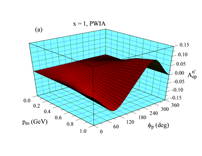
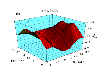
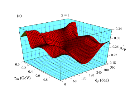
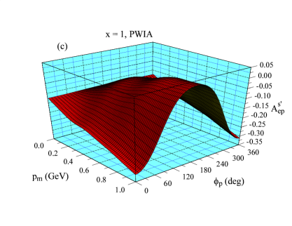
Figure 3: (Color online) The six panels show the three asymmetries that are non-zero in PWIA plotted versus the missing momentum $p_{m}$ and versus the azimuthal angle of the proton, $\phi_{p}$, for a beam energy of $5.5$ GeV, a transferred four-momentum of $Q^{2}=2$ GeV², and $x=1$. We show the PWIA results in the left column (panels a), b), and c)), and the on-shell FSI results in the right column (panels d), e), and f)). The top row shows $A^{n^{\prime}}_{ep}$, the middle row shows $A^{l^{\prime}}_{ep}$, and the bottom row shows $A^{s^{\prime}}_{ep}$. The kinematics are the same as in the previous figure.

We will now turn to the discussion of the off-shell contribution to the FSIs. For $x=1$, the quasi-elastic region, they turn out to be fairly small. This is what we expect, and what we have observed earlier, for the unpolarized case bigdpaper and for a polarized deuteron target targetpol . Therefore, we do not display results for $x=1$, but we move away from the quasi-elastic region, to $x=1.3$, where the off-shell contributions to the FSIs should be a bit larger. In Fig. 4, we show two-dimensional plots of the six asymmetries. The PWIA contribution is shown as the dotted line, the on-shell FSIs are shown by the solid line, and the calculation including the off-shell FSIs is shown by the dashed line. It is again easy to see that FSIs are very important. It also turns out that the off-shell FSIs lead only to modest corrections, and they never lead to qualitative changes in the shape of an asymmetry. The largest effects can be seen in $A^{s^{\prime}}_{p}$, where the value of the asymmetry is reduced significantly for large missing momenta around $p_{m}=0.7$ GeV. For $A^{n^{\prime}}_{ep}$, there is a noticeable increase due to the off-shell FSIs.

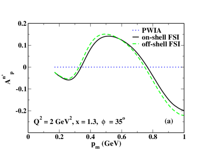
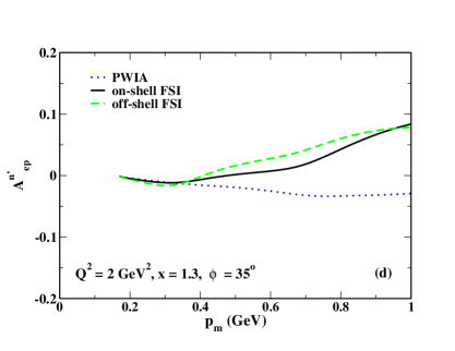
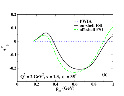
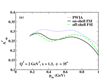
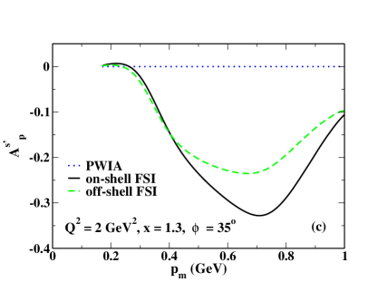
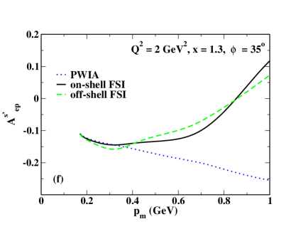
Figure 4: (Color online) The six panels show the six asymmetries plotted versus the missing momentum $p_{m}$ for a beam energy of $5.5$ GeV, a transferred four-momentum of $Q^{2}=2$ GeV², $\phi_{p}=35^{o}$, and $x=1.3$. We show $A^{n^{\prime}}_{p}$ (panel a)), $A^{l^{\prime}}_{p}$ (panel b)), $A^{s^{\prime}}_{p}$ (panel c)), $A^{n^{\prime}}_{ep}$ (panel d)), $A^{l^{\prime}}_{ep}$ (panel e)), and $A^{s^{\prime}}_{ep}$ (panel f)). The curves shown have been calculated in PWIA (dotted), with on-shell FSIs (solid), and including off-shell and on-shell FSIs (dashed).

III.2 Contributions from Individual Parts of the $pn$ scattering amplitude to the FSIs

In our calculation of the final state interactions, we use the full nucleon-nucleon scattering amplitude. There are several ways to decompose and parametrize the $NN$ scattering amplitude. It can be parametrized with five terms: a central, spin-independent term, a spin-orbit term, and three double-spin flip contributions. It can also be given in terms of invariants, using a scalar, vector, tensor, pseudoscalar, and axial term. Some of these parametrizations may be more or less useful and enlightening in trying to understand what is happening. As we are interested in the ejectile polarization, investigating the effects of spin-dependent terms in the FSIs is a logical and interesting step. We separate the NN amplitudes into a central term, a single spin-flip (i.e. spin-orbit) term, and three double spin-flip terms, for details on these Saclay amplitude conventions, see bigdpaper .

In Fig. 5, we show the contributions of the central, central and single spin-flip, and full FSIs to the six asymmetries at $Q^{2}=2$ GeV², $x=1$, and $\phi_{p}=35^{o}$. The clear message from this figure is that a calculation including only central FSIs will fail completely for missing momenta beyond $p_{m}=0.2$ GeV. For the three asymmetries accessible with an unpolarized beam, the central FSI on its own leads to a mostly zero asymmetry, whereas spin dependent FSIs lead to large structures in these observables. For the asymmetries accessible with a polarized electron beam only, the purely central FSI leads to non-zero results for the asymmetries, but the inclusion of spin-dependent FSIs leads to huge changes, both of the shape and size. The differences between the full FSIs and the FSIs without the three double spin-flip terms is largest for $A^{n^{\prime}}_{p}$, where the double spin-flip contribution leads to a broad bump for missing momenta from $p_{m}\approx 0.3$ GeV to $p_{m}\approx 0.8$ GeV. The double spin-flip contributions to $A^{l^{\prime}}_{p}$ are significant as well, leading to an increase in the magnitude of the asymmetry for medium missing momenta. The double spin effects for $A^{s^{\prime}}_{p}$, are smaller, leading to a reduction in magnitude of a small peak at $p_{m}\approx 0.2$ GeV and for large missing momenta, $p_{m}>0.8$ GeV. For the asymmetries that require a polarized beam, the influence of the double spin-flip terms is smaller. There are no huge modifications, and the largest corrections appear for the peak structures around $p_{m}\approx 0.2$ GeV, and for very large missing momenta. This figure gives the impression that an additional polarization, i.e. the beam polarization, may play a similar role as an additional spin-dependence in the FSI, and that at least one of them - either a spin-dependent FSI or a polarized beam - needs to be present to generate an approximately correct ejectile polarization asymmetry. Once the beam is polarized, it seems that introducing the additional double spin-flip terms does not really change the results too much. A very similar picture emerges for $x=1.3$, away from the quasi-elastic peak. The only difference is that the role of the double spin-flip terms becomes even more important for the asymmetries with an unpolarized beam.

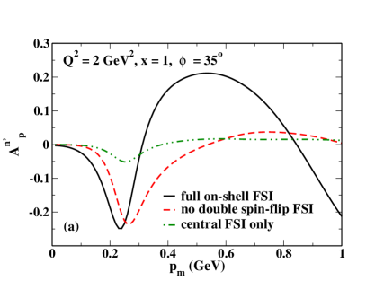
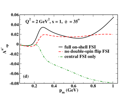
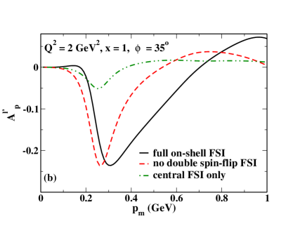
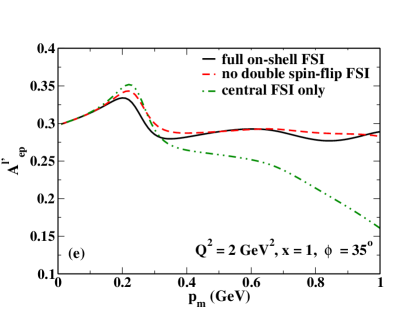
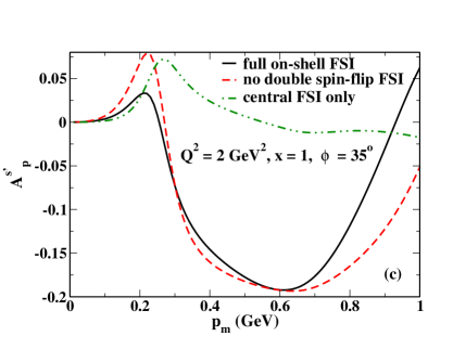
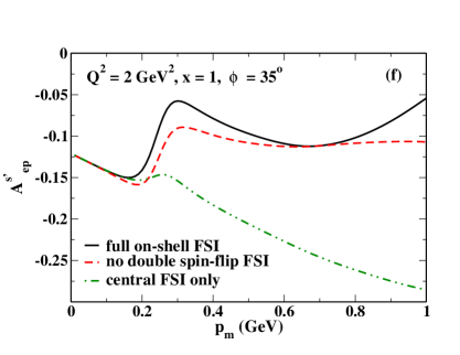
Figure 5: (Color online) The six panels show the six asymmetries plotted versus the missing momentum $p_{m}$ for a beam energy of $5.5$ GeV, a transferred four-momentum of $Q^{2}=2$ GeV², $\phi_{p}=35^{o}$, and $x=1$. We show $A^{n^{\prime}}_{p}$ (panel a)), $A^{l^{\prime}}_{p}$ (panel b)), $A^{s^{\prime}}_{p}$ (panel c)), $A^{n^{\prime}}_{ep}$ (panel d)), $A^{l^{\prime}}_{ep}$ (panel e)), and $A^{s^{\prime}}_{ep}$ (panel f)). The curves shown have been calculated with the full on-shell FSIs (solid), with central and single spin-flip FSIs (dashed), and with central FSI only (dash-dotted).

IV Summary and Outlook

In this paper, we have introduced a formalism for the calculation of asymmetries relevant to a polarized ejectile proton in various frames. In particular, we have presented calculations in a frame relevant to the actual experimental set-up, and avoided any issues with the definition of projection directions in the case that $\theta_{p}=0,\pi$. We have employed a fully relativistic $D(e,e^{\prime}p)$ calculation in impulse approximation. We have used a parametrization of experimental $NN$ data from SAID to describe the full $pn$ scattering amplitude for the final state interaction. This leads to certain limits in the kinematics we can access, as these parametrizations are available only for lab kinetic energies of $1.3$ GeV or less. In our calculations, we have investigated the effects of the different contributions to the NN scattering amplitude: the central, spin-orbit, and double-spin-flip parts.

The asymmetries accessible with an unpolarized beam are zero in PWIA. The influence of the FSIs is very large for all six asymmetries. For the three asymmetries where the PWIA results are non-zero, the FSIs seem to reduce the asymmetries in general, although increases in asymmetries can also be observed for specific kinematics. We have investigated the role played by off-shell FSIs, and they turn out to be fairly small in most situations, with the exception of $A^{s^{\prime}}_{p}$. This is interesting, as the contributions from off-shell FSIs in unpolarized deuteron scattering and for a polarized target were occasionally quite significant. In practice, it is good news that the off-shell FSIs are small, as any remaining theoretical uncertainty is connected to these terms. So, the comparison of our theory to data will be very clean.

We have investigated the role played by different parts of the spin-dependent proton - neutron scattering amplitude in the final state interactions. Using only a central FSI is completely inadequate for all asymmetries. Spin-dependent terms need to be included, and even the double spin-flip contributions are large, in particular for the asymmetries accessible with an unpolarized beam.

Currently, there are no $D(e,e^{\prime}\vec{p})n$ data at high $Q^{2}$ available, but an experiment could easily be performed at Jefferson Lab. In view of the high sensitivity to double spin-flip terms, we feel that one of the most interesting measurements would be to take data for $A^{n^{\prime}}_{p}$ for $x=1.3$, or even for $x=1$. Besides this, measuring ejectile polarization asymmetries for kinematics where unpolarized data or target polarization data are available would allow one to perform a systematic investigation of the reaction mechanism.

Our description of FSIs is complete, but we are still missing the contributions from $\Delta$ isobars and other meson exchange currents. Work on these is in progress.

Acknowledgments: We thank Douglas Higinbotham for discussions on experimental aspects, and for providing us with experimental references. This work was supported in part by funds provided by the U.S. Department of Energy (DOE) under cooperative research agreement under No. DE-AC05-84ER40150 and by the National Science Foundation under grant No. PHY-0653312.

References

- (1) M. Garcon and J. W. Van Orden, Adv. Nucl. Phys. 26, 293 (2001).
- (2) R. A. Gilman and F. Gross, J. Phys. G 28, R37 (2002).
- (3) I. Sick, Prog. Part. Nucl. Phys. 47, 245 (2001).
- (4) J. Ryckebusch, W. Cosyn, B. Van Overmeire and C. Martinez, Eur. Phys. J. A 31, 585 (2007); J. Ryckebusch, P. Lava, M. C. Martinez, J. M. Udias and J. A. Caballero, Nucl. Phys. A 755, 511 (2005); P. Lava, M. C. Martinez, J. Ryckebusch, J. A. Caballero and J. M. Udias, Phys. Lett. B 595, 177 (2004); L. L. Frankfurt, W. R. Greenberg, G. A. Miller, M. M. Sargsian and M. I. Strikman, Z. Phys. A 352, 97 (1995).
- (5) J. Lachniet et al. [CLAS Collaboration], Phys. Rev. Lett. 102, 192001 (2009).
- (6) L. Frankfurt, M. Sargsian and M. Strikman, Int. J. Mod. Phys. A 23, 2991 (2008).
- (7) S. Jeschonnek and J. W. Van Orden, Phys. Rev. C 78, 014007 (2008).
- (8) F. Gross, J. W. Van Orden and K. Holinde, Phys. Rev. C 41, R1909 (1990); F. Gross, J. W. Van Orden and K. Holinde, Phys. Rev. C 45, 2094 (1992).
- (9) R. A. Arndt, W. J. Briscoe, I. I. Strakovsky and R. L. Workman, Phys. Rev. C 76, 025209 (2007); data available through SAID, http://gwdac.phys.gwu.edu/
- (10) M. M. Sargsian, Int. J. Mod. Phys. E 10, 405 (2001); M. M. Sargsian, T. V. Abrahamyan, M. I. Strikman and L. L. Frankfurt, Phys. Rev. C 71, 044614 (2005); L. L. Frankfurt, M. M. Sargsian and M. I. Strikman, Phys. Rev. C 56, 1124 (1997).
- (11) M. M. Sargsian, arXiv:0910.2016 [nucl-th].
- (12) J. Ryckebusch, D. Debruyne, P. Lava, S. Janssen, B. Van Overmeire and T. Van Cauteren, Nucl. Phys. A 728, 226 (2003); D. Debruyne, J. Ryckebusch, W. Van Nespen and S. Janssen, Phys. Rev. C 62, 024611 (2000); B. Van Overmeire and J. Ryckebusch, Phys. Lett. B 650, 337 (2007); W. Cosyn and J. Ryckebusch, arXiv:0904.0914 [nucl-th].
- (13) C. Ciofi degli Atti and L. P. Kaptari, Phys. Rev. C 71, 024005 (2005); C. Ciofi delgi Atti and L. P. Kaptari, arXiv:0705.3951 [nucl-th]; C. Ciofi degli Atti, L. P. Kaptari and D. Treleani, Phys. Rev. C 63, 044601 (2001).
- (14) J. M. Laget, Phys. Lett. B 609, 49 (2005).
- (15) R. Schiavilla, O. Benhar, A. Kievsky, L. E. Marcucci and M. Viviani, Phys. Rev. C72, 064003 (2005).
- (16) Jefferson Lab Experiment E01 - 020, spokespersons W. Boeglin, M. Jones, A. Klein, P. Ulmer, J. Mitchell, E. Voutier.
- (17) K. S. Egiyan et al. [CLAS Collaboration], Phys. Rev. Lett. 96, 082501 (2006); K. S. Egiyan et al. [CLAS Collaboration], Phys. Rev. C 68, 014313 (2003).
- (18) BLAST data from MIT Bates, Ph. D. thesis A. Maschinot (MIT 2005).
- (19) G. Gilfoyle, spokesperson, Jefferson Lab Hall B, E5 run period; G.P. Gilfoyle, (the CLAS Collaboration), ’Out-of-Plane Measurements of the Fifth Structure Function of the Deuteron’, Bull. Am. Phys. Soc., Fall DNP Meeting, DF.00010(2006).
- (20) W. Boeglin, spokesperson, proposal to Jefferson Lab PAC 33, 2007.
- (21) S. Jeschonnek and J. W. Van Orden, Phys. Rev. C 80, 054001 (2009).
- (22) B. Hu et al., Phys. Rev. C 73, 064004 (2006).
- (23) D. Eyl et al., Z. Phys. A 352, 211 (1995).
- (24) B. D. Milbrath et al. [Bates FPP collaboration], Phys. Rev. Lett. 80, 452 (1998) [Erratum-ibid. 82, 2221 (1999)].
- (25) G. Ron et al., Phys. Rev. Lett. 99, 202002 (2007).
- (26) M. K. Jones et al. [Jefferson Lab Hall A Collaboration], Phys. Rev. Lett. 84, 1398 (2000); O. Gayou et al. [Jefferson Lab Hall A Collaboration], Phys. Rev. Lett. 88, 092301 (2002).
- (27) J. Glister et al., Nucl. Instrum. Meth. A 606, 578 (2009).
- (28) R. J. Woo et al., Phys. Rev. Lett. 80, 456 (1998).
- (29) X. Jiang et al. [Jefferson Lab Hall A Collaboration], Phys. Rev. Lett. 98, 182302 (2007).
- (30) J. J. Kelly et al., Phys. Rev. C 75, 025201 (2007).
- (31) A. S. Raskin and T. W. Donnelly, Ann. of Phys. 191, 78 (1989).
- (32) V. Dmitrasinovic and F. Gross, Phys. Rev. C 40, 2479 (1989).
- (33) F. Gross, Phys. Rev. 186, 1448 (1969); Phys. Rev. D 10, 223 (1974), Phys. Rev. C 26, 2203 (1982).