Characterizing steady state and transient properties of reaction-diffusion systems
Abstract
In the past the study of reaction-diffusion systems has greatly contributed to our understanding of the behavior of many-body systems far from equilibrium. In this paper we aim at characterizing the properties of diffusion limited reactions both in their steady states and out of stationarity. Many reaction-diffusion systems have the peculiarity that microscopic reversibility is broken such that their transient behavior can not be investigated through the study of most of the observables discussed in the literature. For this reason we analyze the transient properties of reaction-diffusion systems through a specific work observable that remains well defined even in the absence of microscopic reversibility and that obeys an exact detailed fluctuation relation in cases where detailed balance is fulfilled. We thereby drive the systems out of their nonequilibrium steady states through time-dependent reaction rates. Using a numerical exact method and computer simulations, we analyze fluctuation ratios of the probability distributions obtained during the forward and reversed processes. We show that the underlying microscopic dynamics gives rise to peculiarities in the configuration space trajectories, thereby yielding prominent features in the fluctuation ratios.
pacs:
05.40.-a,05.70.Ln,05.20.-yI Introduction
Understanding general properties of systems that are far from equilibrium remains one of the most challenging problems in contemporary physics. In recent years some remarkable progress has been made in the study of fluctuations in nonequilibrium small systems, see, e.g., Eva93 ; Eva94 ; Gal95 ; Jar97a ; Jar97b ; Kur98 ; Cro98 ; Leb99 ; Cro99 ; Cro00 ; Jar00 ; Hat01 ; Muk03 ; Sei05 ; Spe05 ; Har07 ; Lip02 ; Col05 ; Dou05a ; Wan02 ; Car04 ; Tie06 ; Jou08 ; Ber08 . This progress is mainly due to the formulation of various exact fluctuation and work theorems that provide very generic statements that hold true for large classes of systems. Some of the fluctuation theorems deal with the rate of entropy production, either in systems that are in a nonequilibrium steady state Eva94 ; Gal95 or in systems that initially are in equilibrium before being driven out of equilibrium by an external force Kur98 ; Leb99 . One also distinguishes between detailed Cro99 ; Jar00 ; Sei05 and integral Jar97a ; Hat01 ; Spe05 fluctuation theorems in cases where the system is driven from one steady state to another in finite time. In addition, work theorems Jar97a ; Jar97b ; Cro99 relate the free energy difference between two equilibrium states to the amount of work done during the switching from one state to the other. Many of these theorems have been verified in various experimental settings Lip02 ; Col05 ; Dou05a ; Wan02 ; Car04 ; Tie06 ; Jou08 ; Ber08 , thus illustrating their usefulness for characterizing nonequilibrium systems.
In the past diffusion-limited reaction systems have been proven to be extremely useful in order to understand the generic behavior of many-body systems far from equilibrium. Especially, the study of these systems is at the origin of our understanding of the properties of nonequilibrium phase transitions Hen08 ; Odo08 . Whereas phase transitions in reaction-diffusion systems are by now very well characterized, this is quite different away from these special points. In the present work we discuss different ways of characterizing the steady state and transient properties of generic reaction-diffusion systems, thus contributing to a more comprehensive understanding of these important systems.
Recently discussed extensions of exact fluctuation theorems to nonequilibrium systems with chemical reactions mostly focused on reversible reactions and reaction networks Gas04 ; Sei04 ; And04 ; Sei05a ; And06 ; Sch07 ; And08 . However, many reaction-diffusion models are characterized by irreversible reactions, thus yielding a breaking of the usually assumed microscopic reversibility. By breaking microscopic reversibility we mean that if is the transition probability from configuration to configuration , it can happen that even though . A direct consequence of the absence of microscopic reversibility is that many observables discussed in the context of fluctuation theorems are then ill defined, as in their derivation one explicitly uses that for any path in configuration space the reversed path also exists Cho09 ; Ohk09 . For this reason we focus in our study of fluctuations in reaction-diffusion systems on an observable that is well defined even in the absence of microscopic reversibility. For a system initially in an equilibrium steady state this quantity is identical to the work observable used in the Jarzynski and Crooks relations Jar97a ; Jar97b ; Cro00 .
It should be noted that diffusion-limited systems with effective irreversible reactions can be prepared through a fast evacuation of some of the reaction products. This makes plausible a possible future verification of the intriguing features that are revealed in our study.
In the following we discuss, using a numerical exact method and numerical simulations, steady state and transient properties of various reaction-diffusion systems. Especially, we study fluctuations in systems that are initially in a steady state before being driven away from stationarity by varying one of the reaction rates. This protocol allows us to measure the probability distribution of our observable when going from a steady state , characterized by the value of some reaction rate , to another steady state , characterized by the value of the same reaction rate. Defining the reversed process as changing the reaction rate backwards from to , we can measure also the probability distribution in that case and compare the distributions for the forward and reversed processes. Even though no exact detailed fluctuation theorem is observed for the studied quantity in the absence of detailed balance, we show that the fluctuation ratios display intriguing signatures due to the specific dynamics of the nonequilibrium systems under investigation.
A brief account of some of our results has been given previously Dor09 . In the present paper we not only give a detailed study of the features observed in the ratio of the probability distributions for our observable, we also extend our investigation to other reaction schemes not studied previously. This allows us to gain a better understanding of fluctuations in truly nonequilibrium systems driven away from stationarity and to make the discussion in Dor09 more quantitative.
Our paper is organized in the following way. In the next Section we introduce the different reaction-diffusion models and discuss their steady state properties. In Section III we drive these systems out of stationarity through time-dependent reaction rates. Using an observable that remains well defined even in the absence of microscopic reversibility, we study the probability distributions for this variable and show that the fluctuation ratios formed by the probability distributions computed in the forward and the reversed processes display features which can be related to the dynamical properties of the nonequilibrium system. Finally, Section IV gives our summary as well as an outlook on open problems.
II The models and their steady state properties
We consider one-dimensional lattices made up of sites with periodic boundary conditions where every lattice site can at most be occupied by one particle. Because of the exclusion of multiple occupancy of the lattice sites, a total of configurations exist. Particles are allowed to jump to unoccupied nearest neighbor sites with a diffusion rate and undergo various creation and annihilation reactions. We discuss in the following four basic reaction schemes, see Table 1, and we denote with model 1, 2, 3, and 4 the four models that result from these reaction schemes. In all four models we have an annihilation process, that takes place with rate , as well as a creation process where a new particle is created with rate . The different models differ by the way creation and annihilation take place. Let us first discuss the annihilation process. In models 1 and 2, two particles on neighboring sites undergo a reaction which leads to the destruction of one of the particles. This is different in model 3, where both particles are destroyed at the same time. Finally, in model 4 three neighboring particles are destroyed in the annihilation reaction. For the creation process we note that whereas in models 2, 3, and 4 new particles are spontaneously created at empty sites, in model 1 a new particle can only be created at an empty site if one of the neighboring sites is already occupied.
| model 1 | model 2 | model 3 | model 4 |
|---|---|---|---|
| model 2’ | model 3’ | model 4’ | |
These creation and annihilation processes have been chosen in such a way that the models present different degrees of microscopic reversibility. Thus in model 1 all reactions are reversible, and it is easy to see that this model is in chemical equilibrium for fixed values of the reaction and diffusion rates. Indeed, if both and are different from zero, the reaction scheme reduces to a unique reversible reaction and detailed balance is fulfilled. Model 2, on the other hand, does allow for some reactions to be irreversible. For example, a new particle can be created in the middle of two empty sites, , with rate , but it is not possible to go back immediately to three empty sites as the newly created particle needs a neighbor for the annihilation process to take place. Finally, all reactions are irreversible in models 3 and 4, yielding a complete absence of microscopic reversibility.
We also studied variants of model 2, 3, and 4, called 2’, 3’, and 4’, where we restore microscopic reversibility by allowing the reversed processes to take place with rates and , where , . Even though all reactions are now reversible, these models do not fulfill detailed balance for , and are therefore still nonequilibrium models.
For all our models the dynamics is described by a discrete-time master equation for the probability that the system is in configuration at time Gaspard04 :
| (1) | |||||
Zia and Schmittmann Zia06 ; Zia07 pointed out that for this type of systems a nonequilibrium steady state is characterized by both the stationary probability distribution and the stationary probability currents
| (2) |
between two configurations and .
The stationary probabilities are readily obtained for fixed reaction and diffusion rates by setting up the transition probability matrix W whose elements are the transition rates between different configurations. Of course, as we have configurations for a system of size , the transition probability matrix is a matrix. The stationary probabilities are then obtained as the elements of the null eigenvector of the Liouville matrix L which results when subtracting off the identity matrix from the transition probability matrix. For systems that are small enough this eigenvalue problem can be solved using standard algorithms. For larger system sizes, the stationary probabilities can be measured through standard Monte Carlo simulations.
We show in Fig. 1 the stationary probability distributions for some of the models and various values of the reaction rates. Configurations with the same number of particles are grouped together, with the empty configuration to the left and the fully occupied lattice to the right. The first thing to note is that a change of reaction rates has a large impact on the stationary probability distributions. When the creation of new particles takes place with a small rate, see the black lines in Fig. 1, configurations with only few particles are the most likely. This is different when the creation rate is large, as then configurations with a large number of occupied sites have an increasing weight, see the cyan (light gray) lines in Fig. 1. A corresponding behavior is observed when changing the rate . On the other hand, however, a change of the value of the diffusion constant mainly changes the distributions quantitatively, see Fig. 1(c) and (d).
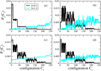
Even though there are visible differences in the stationary probability distributions between Fig. 1(a) and (c), it is not possible to guess from these stationary probabilities alone whether the system is in equilibrium, as it is the case for model 1, or whether we are dealing with a nonequilibrium system with a fully irreversible reaction scheme, as for model 3. The stationary probability distribution does not allow by itself to characterize unequivocally nonequilibrium steady states.
Instead of analyzing one-by-one the stationary probability currents for various configuration pairs, it is more convenient to look at the global quantity Pla09
| (3) |
In Fig. 2(a) we show the dependence of on the value of the creation rate for fixed values of and . Obviously, the dependence is very different for the different models. In the equilibrium model 1 one does not have any non-vanishing stationary probability currents, and is zero for all values of the reaction and diffusion rates, as expected. This is different for the nonequilibrium systems which are characterized by non-vanishing stationary probability currents. Interestingly, the value of decreases in model 2 for larger , whereas for models 3 and 4 it increases as a function of . In order to understand this difference in behavior, we recall that for larger values of configurations with a large number of particles have an increased stationary probability. As a result, free sites will have with high probability occupied neighboring sites, and the creation process effectively equals the process . This is, however, exactly the reversed reaction to the annihilation process of model 2, which explains why for large the behavior of model 2 approaches that of an equilibrium system. For models 3 and 4, however, all reactions remain irreversible and keeps on growing.
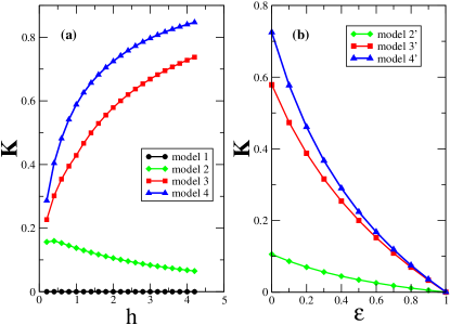
In Fig. 2(b) we plot as a function of the parameter for the modified models 2’, 3’, and 4’ for which we allow the reversed reactions to take place. As a result, all reactions are now reversible, but for all cases we are still out of equilibrium as long as . Increasing decreases the distance to equilibrium which is finally reached for when all reactions and the corresponding reversed reactions are taking place with the same rate.
This discussion of the stationary probability distributions and of the stationary probability currents shows that it is not possible to characterize in an unambiguous way a nonequilibrium system solely through its stationary probability distribution. Much information is contained in the stationary probability currents which do allow to distinguish between the properties of equilibrium, weakly nonequilibrium, and strongly nonequilibrium systems. Therefore these currents allow to quantify the distance to equilibrium, making them a useful tool for the characterization of nonequilibrium systems.
III Transient fluctuation relations
Having discussed the steady-state properties of reaction-diffusion models, we now focus on the characterization of the transient behavior when the systems are brought out of stationarity and are then allowed to relax to a new steady state. We are realizing this through a protocol in which we change one of the reaction rates. Experimentally, a change of rates of chemical reactions can be achieved by changing the temperature, for example. In our protocol we change one of the rates from an initial value to a final value in equidistant steps of length , yielding for the reaction rate the values with . We assume that at every step only one reaction or diffusion process takes place.
In the following we discuss mainly numerical exact results for small one-dimensional systems. This numerical exact approach is rather straightforward and is summarized in the Appendix. Larger systems can be studied along the same lines through numerical simulations, but this must be done with some care in order to guarantee a sufficient sampling of rare events Dor10 .
III.1 Observables
We discuss in the following two observables which differ by the fact that for one of the variables microscopic reversibility has to be assumed whereas for the other no such assumption has to be made. For a system that is microscopic reversible, as for example a system that fulfills detailed balance, we will discuss the difference between these two quantities explicitly.
In order to define these quantities let us first suppose that the system is in a steady state. Starting from a configuration , the system is in the configuration at step , such that after steps the system has performed the following path in configuration state: . The probability for this path is
| (4) |
where is the transition probability from configuration to configuration . Denoting the reversed path by , one then defines for Markovian systems the quantity Leb99 ; Sei05a
| (5) |
When the system is driven out of stationarity, we can generalize this definition to a time dependent reaction rate, yielding
| (6) |
where is the probability to find the configuration in the stationary state corresponding to the value of the reaction rate and is the transition probability from to at step .
A closer look at the observable reveals that its definition requires that if than also has to be non zero. However, in some of our reaction-diffusion models this condition is not fulfilled as microscopic reversibility is broken, and we can not use to study them. Hatano and Sasa Hat01 have proposed a different quantity that is closely related to , but that does not assume microscopic reversibility. Adapting this quantity for systems driven out of stationarity, we can write it in the following way Dor09
| (7) |
The quantity has been called the driving entropy production in Esp07 .
For a system with microscopic reversibility we can derive a relation between and . With the help of the probability current
| (8) | |||||
we can write Eq. (7) for in the following form:
| (9) | |||||
which reveals that the difference between and is composed of terms which have very different physical origins. The first term in the in Eq. (9) is due to non-vanishing probability currents between different configurations and is therefore characteristic for nonequilibrium states. The second term is non-trivial only in transient processes as it accounts for a shift in the reversed transition probability. This term reduces to the trivial value 1 in case one remains in a given steady state, with for all . If this steady state is in addition an equilibrium state, the probability currents are all vanishing, and one has .
It is easy to show Hat01 ; Sei05 ; Esp07 that for transient processes both quantities fulfill an integral fluctuation theorem: and , where the average is taken over all possible histories when driving the system out of a general steady state. For a system that is initially in an equilibrium steady state the relation reduces to the Jarzynski relation Jar97a as then , where is the work done on the system, is the free energy difference between initial and final states, and is the inverse temperature. The difference is the dissipative work.
III.2 Probability distributions
In systems with detailed balance, an exact fluctuation relation is obtained when plotting the ratio between the probability distributions and of the dissipative work done on the system in the forward and reversed processes Cro00 :
| (10) |
Recalling that for systems with detailed balance we have the identity , it is tempting to ask whether for an exact fluctuation theorem like (10) can also be encountered for a system initially in a nonequilibrium steady state. In fact, this is not the case: the absence of detailed balance in a nonequilibrium steady state entails non-zero probability currents, and no simple relation like the relation (10) exists for in this case. As we shall discuss below, the corresponding fluctuation ratios yield systematic deviations from the simple behavior encountered in systems with detailed balance, these deviations containing non-trivial information on the nonequilibrium system at hand.
However, before analyzing these ratios of probability distributions, we shall first discuss the probability distributions themselves.
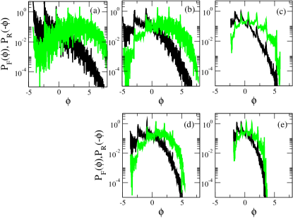
Figures 3-6 show typical examples for the probability distributions of and when changing the creation rate from an initial value to a final value in steps (we only show the case of a varying creation rate , but the following discussion can be made along similar lines when changing the value of the annihilation rate ).
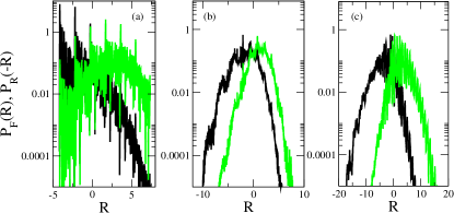
Fig. 3 shows the probability distributions of for three cases that fulfill microscopic reversibility:
models 1, 2’, and 3’.
These different probability distributions are not Gaussian but are characterized by a rather irregular structure.
Their shape depends on the dynamics of the different models, expressed by the different reaction schemes.
It is, however, not straightforward to relate specific features of the probability distributions to
the different reactions.
It is important to note that the peaks dominating these distributions do not have their origin
in the noisiness of some numerical data, but are real as
we are using a numerically exact method. In addition, our numerically exact method also allows us to circumvent
any issues that might appear due to an insufficient sampling of rare events. This will be of importance in the
next section when we discuss the ratios of the forward and reversed probability distributions.
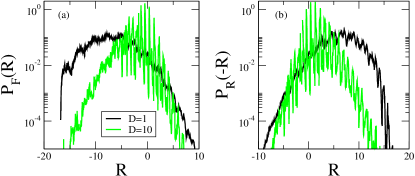
The probability distributions show a strong dependence on the system parameters. This is illustrated in Fig. 4 where we compare for model 3’ the distributions obtained for different values of the diffusion rate. When we increase the diffusion rate, the general shape of the probability distribution changes and, in addition, a large number of distinct peaks appear.
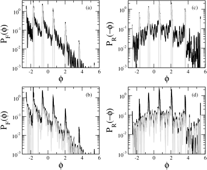
The probability distributions for differ markedly from those for , see Fig. 5. This was expected as the main difference between both quantities are the probability currents which are non-zero for a system that is out of equilibrium. It is only for the equilibrium model 1 that the distributions for both quantities are similar. Interestingly, the probability distributions for for both the forward and reversed processes are characterized by the presence of prominent peaks. An increase of the diffusion constant strongly amplifies these peaks but does not change the overall shape of the probability distributions. The fact that the heights of the peaks depend on the value of the diffusion constant indicates that these peaks are related to trajectories in configuration space that are dominated by diffusion steps and not by reactions. In Fig. 6 we verify for model 3 that the main contributions to the peaks for a drive of length indeed come from the trajectories where only diffusion takes place such that the number of particles is constant along these trajectories. The subleading contribution, also shown in Fig. 6, comes from the trajectories where a single reaction takes place which changes the number of particles in the system. Because the peaks are dominated by trajectories with pure diffusion, the positions of the peaks are the same for the forward and reversed processes, the leftmost peak resulting from the diffusion of a single particle in the system, whereas the rightmost peak is due to the diffusion of a single empty site in the system.
Before closing this section, we remark that in Esp07 similar peaks have been observed in the probability distributions of the driving entropy production as well as of other related quantities in a model for electron transport through a single level quantum dot.
III.3 Fluctuation ratios
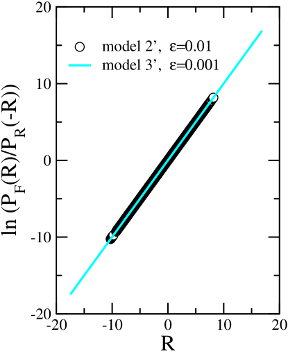
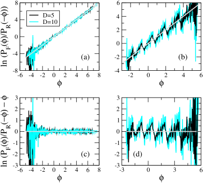
Having just discussed the probability distributions of the quantities and , we now move on and study the fluctuation ratios formed by these probability distributions. For a system driven out of an initial equilibrium state and fulfilling detailed balance, Crooks has shown the exact relation (10) to exist between the probability distributions of the dissipative work measured in the forward and time-reversed processes. This remarkable result can be extended to systems that are still reversible microscopically but that do not fulfill detailed balance any more Har07 . As illustrated in Fig. 7 for models 2’ and 3’, the ratios of the probability distributions for show a simple exponential dependence on . The perfect exponential obtained from our data nicely validates our numerical exact approach. Obtaining a plot of similar quality through Monte Carlo simulations is difficult as rare events are then hard to measure.
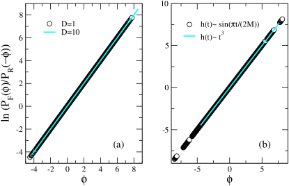
Even though in the absence of microscopic reversibility is ill defined, this is different for as this quantity exclusively involves the steady-state probabilities, see Eq. (7). For an equilibrium system fulfills an exact fluctuation theorem as it then reduces exactly to the dissipative work. As shown in Fig. 8 for model 1, an exponential relation is indeed obtained for all parameter values as well as for different driving processes .
However, for a system with nonequilibrium steady states no exponential detailed fluctuation relation is expected for as this quantity does not contain the information on nonequilibrium currents, see Eq. (9). We show in Fig. 9 ratios of the probability distributions of for models 2 and 3. For model 2 the deviations from the exponential are random and no pronounced dependence on system parameters, as for example the diffusion rate , is observed. For model 3, however, a qualitatively different behavior is encountered and systematic deviations in the form of oscillations are observed. Similar oscillations are also observed for model 4 where three neighboring particles are destroyed in the annihilation process. Interestingly, the amplitudes of these oscillations increase for increasing diffusion rates. At first one might think that this increase in peak height when increasing should be related to the increase of the peaks in the probability distributions themselves, see the discussion in the previous section. However, this is too simplistic as an increase of peak heights in the probability distributions is also observed for models 1 and 2 for which we do not observe the corresponding behavior in the fluctuation ratios. What is different between models 1 and 2 on the one hand and models 3 and 4 on the other hand is that for the former models any change in the forward and reversed probability distributions is compensated when forming the ratio (this compensation is exact for model 1 and approximate for model 2), whereas for the latter models this compensation is only partial, such giving rise to peaks also in the fluctuation ratios.
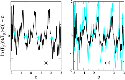
Before discussing the origin of this difference, let us first have for model 3 a closer look at the peaks in the fluctuation ratio. We first note that the positions of these peaks are not identical to the positions of the extrema in the probability distributions (see for example Fig. 6). In Table 2 we compare the positions of the maxima and minima in the fluctuation ratio with the peak positions in the probability distributions. The observed offset means that the peaks in the probability distributions for the forward and reversed processes compensate each other when forming the ratio, but that the compensation is only partial away from the peaks. Recalling that the peaks result from trajectories in configuration space with only diffusion steps and that trajectories with reactions make up the part between the peaks, we can conclude that reactions are responsible for the peaks in the fluctuation ratios. In order to verify this assumption we analyzed the contributions to the fluctuation ratio coming from the different types of trajectories. We show in Fig. 10 that the observed minima and maxima are indeed mainly due to the trajectories with a single reaction process. For this we compare the fluctuation ratio with the quantity where is the probability distribution for all trajectories having (a) only diffusion steps or (b) exactly one reaction process. Obviously, the peaks in the latter ratio coincide with the peaks in the fluctuation ratio.
| PD maxima | FR maxima | FR minima |
| 0.60 | 0.50 | 0.82 |
| 2.02 | 1.89 | 2.25 |
| 3.64 | 3.44 | 3.84 |
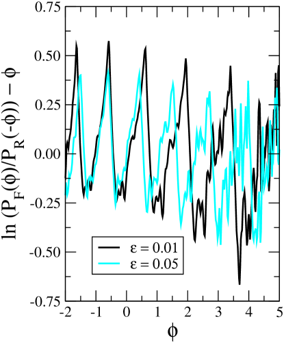
As a second interesting observation we note that the oscillations in the fluctuation ratios are not restricted to cases where microscopic reversibility is broken but are much more widespread. As is shown in Fig. 11 for model 3’ (the same holds for model 4’) peaks in the fluctuation ratios also show up in some systems where all reactions are reversible.
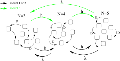
In order to understand the origin of these oscillations we need to go back to the different reaction schemes summarized in Table 1. The configuration space of a reaction-diffusion system can be thought to be composed of smaller units formed by the configurations with a common number of particles. A diffusion step conserves the number of particles, thereby connecting two configurations in the same unit. A passage from one unit to another always involves a change of particle number and is therefore exclusively due to a reaction process. This is sketched in Fig. 12. Keeping this in mind, a fundamental difference emerges between models 1 and 2 on the one hand and models 3 and 4 on the other hand. In the former systems every reaction changes the particle number by 1, . In the latter systems, however, also larger changes in the particle number happen in the annihilation process, with for model 3 and for model 4. As a consequence, loops in configuration space that connect a unit with constant with itself and that involve reactions will display an asymmetry in the number of creation and annihilation processes. Thus for model 3 the smallest loop contains two creation processes and one annihilation. This effect is still present, even though in a weaker form, when we add the backreactions and end up with a microscopically reversible model like model 3’ with a variable number of particles added or subtracted in the different reactions. It is this difference in the number of particles created in a creation process or destroyed in an annihilation event that yields contributions to the probability distributions which are not compensated in the fluctuation ratio.
IV Discussion
Characterizing the out-of-equilibrium properties of interacting many-body systems remains one of the most challenging tasks in contemporary physics. The recent advent of exact fluctuation and work theorems yielded some excitement in the community as it indicated a possible way of characterizing large classes of nonequilibrium systems.
In our work we try to characterize diffusion-limited reactions both in their nonequilibrium steady state and in the transient state when the systems are driven out of stationarity. For systems in their steady state we confirm the expectation that probability currents allow to distinguish between equilibrium and nonequilibrium steady states. In addition, they also allow to define a global quantity that quantifies the distance to equilibrium. This way of characterizing nonequilibrium steady systems remains valid even when microscopic reversibility is broken, as it is the case for many reaction-diffusion systems.
The situation is more complicated if one wishes to characterize reaction-diffusion systems through fluctuation and work theorems. If one studies a system for which microscopic reversibility is fulfilled, one can define a work-like quantity, our quantity , see eq. (6), for which exact detailed fluctuation theorems not only hold in the steady states but are also valid when the system is driven out of stationarity through time dependent reaction rates. In absence of microscopic reversibility, however, can not be used as it is no longer well defined. Instead we propose to use the driving entropy production , see eq. (7), initially introduced in Hat01 ; Esp07 , as this quantity exclusively uses stationary probabilities and therefore remains well defined even in the absence of microscopic reversibility. Whereas the driving entropy production always fulfills a global fluctuation theorem Hat01 ; Esp07 , it only fulfills a detailed fluctuation theorem for systems with equilibrium steady states. At first look, this seems to strongly reduce the usefulness of his quantity for the characterization of systems with nonequilibrium steady states. However, as we showed in this paper, the deviations of the fluctuation ratios for from a simple exponential behavior do contain non-trivial information on the trajectories in configuration space. Indeed, in cases where the change in the number of particles is different for different reactions, we observe systematic deviations from a simple exponential behavior. These deviations, which take the form of peaks superimposed on an exponential, mainly result from trajectories in configuration space where exactly one reaction takes place.
It is not an easy task to quantitatively relate the peak heights and the peak positions to the values of the system parameters. For this, a much more in-depth study is needed where all the parameters are varied in a systematic way Dor10 .
Whereas the driving entropy production remains a well-defined quantity even in the absence of microscopic reversibility, we need to mention that in many cases this could be a quantity that is difficult to measure as the knowledge of the stationary probability distribution of the system is required. As a consequence, the practical importance of could be restricted, especially for experimental systems where the stationary probability distribution is often not easily accessible.
How general are the results found in this work? Based on the reaction schemes discussed in this work and given in Table 1, we expect the peaks to appear in the fluctuation ratios for for any reaction-diffusion system that allows for a variable number of particles to be created or destroyed in the different reactions. This also encompasses more complicated systems with two or more particle types. In addition, signatures of the same type should also be observed for other system classes with a configuration space topology that is similar to that of the the reaction-diffusion systems (i.e., composed by groups of configurations that are only connected in a very specific way) and with a similar asymmetry in the configuration space trajectories. An extension of our work along these lines is planed for the future.
Acknowledgements.
We thank Chris Jarzynski and Frédéric van Wijland for interesting and stimulating discussions. This work was supported by the US National Science Foundation through DMR-0904999.Appendix
In order to compute the probability distribution of , see (7), when changing some rate from its initial value to the final value in steps, with , , we first need to know the stationary probability distributions for any value . This is easily done by determining the null eigenvector of the Liouville matrix. We then need to generate all possible sequences of configurations (paths in configuration space) , where only one reaction or diffusion takes place at every step. Starting form every possible initial configuration, we have to built up a tree structure to all the configurations that can be reached in steps with non-zero probability. This is done recursively by a standard depth-first search algorithm that ends when we reach the th step. We now have to attach a probability to every one of these generated paths. For this we are multiplying the probability to select the initial configuration with the product of the transition probabilities:
| (11) |
Having now determined every path and its probability, we need in addition the values of along these different paths, which we obtain through the equation
| (12) |
where is the stationary probability to find the configuration at the value of the rate . Putting everything together, the probability distribution is finally obtained through the expression
| (13) |
In addition to the just described forward process we also study the reversed process where we start in configuration with the rate before changing the reaction rate in steps to its final value . The probability distribution for this process is then
| (14) |
with
| (15) |
In Section III we discuss not only the quantity but also the quantity defined by Eq. (6). For this second quantity the procedure is exactly the same, only the calculation of the values of for the different paths has to be replaced by the values of .
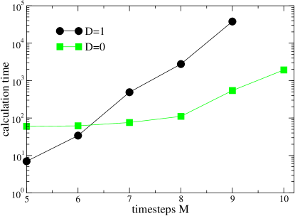
This numerical exact approach is limited to small system sizes and few steps , as the number of paths grows exponentially with both and , see Fig. 13. For example, for the number of paths increases from 404 for to 8.6 for .
References
- (1) D. J. Evans, E. G. D. Cohen, and G. P. Morriss, Phys. Rev. Lett. 71, 2401 (1993).
- (2) D. J. Evans and D. J. Searles, Phys. Rev. E 50, 1645 (1994).
- (3) G. Gallavotti and E. G. D. Cohen, Phys. Rev. Lett. 74, 2694 (1995).
- (4) C. Jarzynski, Phys. Rev. Lett. 78, 2690 (1997).
- (5) C. Jarzynski, Phys. Rev. E 56, 5018 (1997).
- (6) J. Kurchan, J. Phys. A 31, 3719 (1998).
- (7) G. E. Crooks, J. Stat. Phys. 90, 1481 (1998).
- (8) J. L. Lebowitz and H. Spohn, J. Stat. Phys. 95, 333 (1999).
- (9) G. E. Crooks, Phys. Rev. E 60, 2721 (1999).
- (10) G. E. Crooks, Phys. Rev. E 61, 2361 (2000).
- (11) C. Jarzynski, J. Stat. Phys. 98, 77 (2000).
- (12) T. Hatano and S.-I. Sasa, Phys. Rev. Lett. 86, 3463 (2001).
- (13) S. Mukamel, Phys. Rev. Lett. 90, 170604 (2003).
- (14) U. Seifert, Phys. Rev. Lett. 95, 040602 (2005).
- (15) T. Speck and U. Seifert, J. Phys. A 38, L581 (2005).
- (16) R. J. Harris and G. M. Schütz, J. Stat. Mech. P07020 (2007).
- (17) J. Liphardt, S. Dumont, S. B. Smith, I. Tinico, Jr., and C. Bustamante, Science 296, 1832 (2002).
- (18) D. Collin, F. Ritort, C. Jarzynski, S. B. Smith, I. Tinico, Jr., and C. Bustamante, Nature (London) 437, 231 (2005).
- (19) F. Douarche, S. Ciliberto, A. Petrosyan, and I. Rabbiosi, Europhys. Lett. 70, 593 (2005).
- (20) G. M. Wang, E. M. Sevick, E. Mittag, D. J. Searles, and D. J. Evans, Phys. Rev. Lett. 89, 050601 (2002).
- (21) D. M. Carberry, J. C. Reid, G. M. Wang, E. M. Sevick, D. J. Searles, and D. J. Evans, Phys. Rev. Lett. 92, 140601 (2004).
- (22) C. Tietz, S. Schuler, T. Speck, U. Seifert, and J. Wrachtrup, Phys. Rev. Lett. 97, 050602 (2006).
- (23) S. Joubaud, N. B. Garnier, and S. Ciliberto, EPL 82, 30007 (2008).
- (24) J. Berg, Phys. Rev. Lett. 100, 188101 (2008).
- (25) M. Henkel, H. Hinrichsen, and S. Lübeck, Non-Equilibrium Phase Transitions: Volume 1: Absorbing Phase Transitions (Springer/Dordrecht and Canopus/Bristol, 2008).
- (26) G. Ódor, Universality in Nonequilibrium Lattice Systems: Theoretical Foundationa (World Scientific/Singapore, 2008).
- (27) P. Gaspard, J. Chem. Phys. 120, 8898 (2004).
- (28) U. Seifert, J. Phys. A 37, L517 (2004).
- (29) D. Andrieux and P. Gaspard, J. Chem. Phys. 121, 6167 (2004).
- (30) U. Seifert, Europhys. Lett. 70, 36 (2005).
- (31) D. Andrieux and P. Gaspard, Phys. Rev. E 74, 011906 (2006).
- (32) T. Schmiedl and U. Seifert, J. Chem. Phys. 126, 044101 (2007).
- (33) D. Andrieux and P. Gaspard, Phys. Rev. E 77, 031137 (2008).
- (34) S.-H. Chong, M. Otsuki, and H. Hayakawa, preprint arXiv:0906.1930.
- (35) J. Ohkubo, preprint arXiv:0909.5292.
- (36) S. Dorosz and M. Pleimling, Phys. Rev. E 79, 030102(R) (2009).
- (37) P. Gaspard, J. Stat. Phys. 117, 599 (2004).
- (38) R. K. P. Zia and B. Schmittmann, J. Phys. A 39, L409 (2006).
- (39) R. K. P. Zia and B. Schmittmann, JSTAT P07012 (2007).
- (40) T. Platini and R. K. P. Zia, private communication.
- (41) S. Dorosz amd M. Pleimling, unpublished.
- (42) M. Esposito, U. Harbola, and S. Mukamel, Phys. Rev. E 76, 031132 (2007).