The strong form of the Levinson theorem for a distorted KP potential

Abstract

We present a heuristic derivation of the strong form of the Levinson theorem for one-dimensional quasi-periodic potentials. The particular potential chosen is a distorted Kronig-Penney model. This theorem relates the phase shifts of the states at each band edge to the number of states crossing that edge, as the system evolves from a simple periodic potential to a distorted one. By applying this relationship to the two edges of each energy band, the modified Levinson theorem for quasi-periodic potentials is derived. These two theorems differ from the usual ones for isolated potentials in non-relativistic and relativistic quantum mechanics by a crucial alternating sign factor $(-1)^{s}$, where $s$ refers to the adjacent gap or band index, as explained in the text. We also relate the total number of bound states present in each energy gap due to the distortion to the phase shifts at its edges. At the end we present an overall relationship between all of the phase shifts at the band edges and the total number of bound states present.

I Introduction

There has been a great revival of interest in one-dimensional condensed matter systems in recent years. The technological advances in the construction of quasi one-dimensional hetero-structures have provoked a great deal of theoretical research, investigating the transmission and reflection coefficients wave1 ; wave2 ; amp1 ; wave3 ; amp4 ; wave7 ; wave5 ; amp2 ; amp3 ; amp5 ; amp6 ; wave6 ; wave4 ; asr1 ; asr2 ; asr3 ; amplitp ; ra1 ; amplitM , energy band structures asr1 ; asr2 ; asr3 , and pattern of resonant states asr1 ; asr2 ; asr3 ; ra1 ; r2 of one-dimensional periodic systems. The effects of impurities and defects in super-lattices have also been studied widely impu0 ; impu1 ; impu2 ; impu10 ; impu3 ; impu4 . The impurities, although unwanted in some cases, are found to be extremely useful in some other cases like energy pass filters, quantum wires, and waveguides impu1 ; impu2 ; impu3 ; impu10 . There have also been studies on the total number of bound states and its relation to the number of bound states of each constituting potential fragment impu5 ; impu6 ; impu7 ; impu8 ; impu9 . A Levinson theorem has been derived and used to study this relation in some works impu5 ; impu6 .

The Levinson theorem for simple non-relativistic quantum mechanical systems, in its original form Levi , gave a relationship between the $S$-state scattering phase shift $\delta_{0}(k)$ and the total number of zero-angular-momentum bound states $n_{0}$,

$$\delta_{0}(0)-\delta_{0}(\infty)=\pi n_{0}.$$ (1)

In 1957 Jauch Jauch gave an alternative proof of Eq. (1) and generalized it to any angular momentum state,

$$\delta_{l}(0)-\delta_{l}(\infty)=\pi n_{l}.$$ (2)

He also showed that the above relationship is a simple consequence of the orthogonality and the completeness of the eigenfunctions of the full Hamiltonian. In 1960 Newton Newton showed that when the potential is such that there exists a threshold bound state with $l=0$, the statement of the Levinson theorem needs to be modified to

$$\delta_{0}(0)-\delta_{0}(\infty)=\pi\left(n_{0}+\frac{1}{2}\right).$$ (3)

A threshold bound state is most easily understood as a state with zero momentum such that if the attractiveness of the potential is increased infinitesimally, that state would emerge as a true bound state. Much work in the literature has been devoted to the proof of Levinson’s theorem by different methods and its generalization to scattering by non-spherically symmetric N2 or nonlocal potentials (for a review see for example ref. rev and the references cited there). For an elegant new derivation see Boya .

In $1993$ a strong form of the Levinson theorem was presented in the context of relativistic quantum mechanics in two space-time dimensions stronglev0 ; stronglev1 . The model considered consisted of a Dirac particle coupled to a pseudo-scalar background field in a solitonic configuration. The strong form of the Levinson theorem related the phase shifts at each boundary of the continua $E=\{\pm m,\pm\infty$ } to the number of bound states that cross that particular boundary, as the soliton evolves from the trivial background. Moreover it was shown that the presence of the soliton makes the phase shifts nontrivial at $E=\pm\infty$. The strong form of the Levinson theorem for the finite boundaries of the continua states that

$$\left.\delta(E)\right|_{E=\pm m}=(N_{exit}-N_{enter})\pi$$ (4)

where $N_{exit}$ and $N_{enter}$ denote the number of bound states that exit or enter the continuum from that edge, as the soliton or any other disturbance is formed, respectively. Any threshold bound state involved in this process counts as one half. That is, $N_{exit}$ could involve a threshold bound state in two ways: either a threshold bound state which turns into a complete bound state, or a threshold bound state which appears at the band edge originating from the continuum, as a distortion is formed. Similarly $N_{enter}$ could involve a threshold bound state in two ways which are exact opposites of the ones explained above. A relationship analogous to Eq.(4) was also derived for the infinite boundaries, which differs from it only by a minus sign. If parity is a symmetry of the problem, the above statements are true for each sign of parity separately. Combining these statements, one can easily obtain the Levinson theorem for the Dirac equation:

$$\Delta\delta\equiv[\delta^{sky}(0)-\delta^{sky}(\infty)]+[\delta^{sea}(0)-\delta^{sea}(\infty)]$$

$$=\pi\left(\mathcal{D}^{sky}+\mathcal{D}^{sea}\right)=\pi\mathcal{D}=(N+\frac{N_{t}}{2}-\frac{N_{t}^{0}}{2})\pi,$$ (5)

where $\mathcal{D}$ denotes the total spectral deficiency, and superscripts $sky$ or $sea$ denote the Dirac sky or sea, respectively. $N$ is the total number of true bound states, $N_{t}$ is the total number of threshold bound states at the given strength of the potential, and $N_{t}^{0}$ is the total number of threshold bound states at the zero strength of the potential, which is generically non-zero in one-dimensional systems. The spectral density in both of the continua, their position dependent deficiencies, and the local and global completeness of the total spectrum in the presence of the solitons were explicitly shown in nuclear . We should mention that there has been further works on the strong form of the Levinson theorem, see for example stronglev2 ; stronglev3 . It is interesting to note that, when the $E<0$ part is eliminated, both forms of the Levinson theorem are also true in non-relativistic quantum mechanics for isolated potentials, although the distinction between the two forms is blurred by the fact that $\delta(\infty)$ can be usually set to zero in problems of physical interest.

In $1966$ Callaway Callaway derived a form of the Levinson theorem for the scattering of an excitation in a solid by a potential of finite range,

$$\delta(E_{s}^{l})-\delta(E_{s}^{u})=\pi n_{s},$$ (6)

where $\delta(E_{s}^{l})$ and $\delta(E_{s}^{u})$ are the phase shifts at the lower and upper energy edges of the $sth$ band, respectively, and $n_{s}$ is the number of the states forced out of the band by the perturbation. The quantity $n_{s}$ is exactly the same as the spectral deficiency in the $s$th energy band, which can be denoted by $\mathcal{D}_{s}$. The spectral deficiency can be simply defined as the difference between the total number of states in the presence and absence of the distortion. Due to recurring interest in one-dimensional systems, this theorem has been derived and applied to finite one-dimensional potentials where the half-bound states are also taken into account impu5 ; impu6 ; 1dlev3 ; 1dlev4 ; 1dlev5 ; 1dlev6 ; 1dlev7 ; 1dlev8 . However, as we shall show, Eq. (6), which is identical to its counterparts in non-relativistic and relativistic quantum mechanics for isolated potentials, is not always true and needs several modifications. In this paper we obtain both forms of the Levinson theorem for one-dimensional quasi-periodic potentials, which, to the best of our knowledge, have not been presented before. Moreover, we compare both forms to their analogues for isolated potentials. Since this form of the Levinson theorem for quasi-periodic cases is presented about 60 years after Levinson s original derivation, we believe a simple illustration should suffice. We hope to present its rigorous derivation later on.

As far as we know, the prevailing misconception is that the form of the Levinson theorem for periodic potentials is exactly the same as its form for isolated potentials. Here we present a heuristic derivation of the strong form of the Levinson theorem for one-dimensional quasi-periodic potentials, which we believe could clear up this misconception. In order to obtain the correct form of the Levinson theorem for the solid state of matter, in particular its strong form, we investigate the simplest non-trivial, yet exactly solvable model, which is a distorted Kronig-Penney (KP) model. This choice has the advantage of making the derivation of the new forms of this theorem clear and simple. Moreover, although the KP model krng1 is very simple and has been discussed in many solid state textbooks, its generalizations have found wide usage in investigating the essential features of more complex or experimentally important structures such as super-lattices krng2 ; krng3 ; krng4 ; krng5 ; krng6 ; krng7 ; krng8 . For this reason, new methods are still being introduced to study the energy band structure and eigenfunctions of KP models krng9 ; krng10 ; krng11 ; krng12 ; krng13 . Therefore, this investigation can also illuminate the essential features of the Levinson theorem in more realistic models of solids.

To start the heuristic derivation we need to fully investigate the physical properties of the undistorted system which is the simple KP. However, since these are included in the standard textbooks we shall do so very briefly, mainly to introduce our notation. In Section two, we find the wave functions and energy band structure for the simple KP model. However we discuss the parity eigenvalues of states at the band edges in more detail, since the parity assignments will be crucial for obtaining of the Levinson theorem. We also discuss the criteria for the appearance of resonant states within the bands and their effects on the parities of the states at the band edges. In section three we calculate the bound states, scattering states and their phase shifts for a distorted KP model. The system has infinite spacial extent, and an infinite number of bound states. However one can still define the phase shifts directly from the scattering states (continuum eigenstates) of the full Hamiltonian wang ; sprung . As we shall show, the phase shifts have the correct limiting form in the sense that as the distortion disappears the phase shifts go to zero. The phase shifts also correctly count the bound states in the energy gaps and the spectral deficiencies in the bands, exactly as one would expect from the Levinson theorem. In this derivation we do not need to start with a truncated form of the potential weber1 ; weber2 . Moreover it is shown that there exists a strong form of the Levinson theorem which relates the phase shifts at each band edge to the number of bound states crossing that edge and the gap index, as the distortion is formed. Then the relationship between the difference of the phase shifts at the edges of a given energy band is related to the spectral deficiency in that band and its index. These relationships constitute modified forms of the Levinson theorem for the distorted KP model. An additional relationship between the phase shifts at the boundaries of any gap and the number of bound states in that gap is also obtained.

II Essential Features of the Simple Kronig-Penney model

II.1 Eigenfunctions

The KP potential chosen is comprised of barriers of width $2a$ and height $V_{3}$, and wells of width $2b$. The lattice period is thus $l=2(a+b)$, as shown in Fig. 1. For the simple KP model $\Delta V$ shown in the figure is zero. The solution to the Schrödinger equation for this simple model is,

$$\psi(x_{n})=\left\{\begin{array}[]{cc}A_{n}e^{ik_{2}(x_{n}-nl)}+B_{n}e^{-ik_{2}(x_{n}-nl)}\hskip 5.69054ptn\mbox{\small th well},\\ C_{n}e^{ik_{3}(x_{n}-nl)}+D_{n}e^{-ik_{3}(x_{n}-nl)}\hskip 5.69054ptn\mbox{\small th barrier},\\ \end{array}\right.$$ (7)

where,

$$n\mbox{\small th well} := [(n-1)l+a]\leq x_{n}\leq nl-a,$$ (8)

$$n\mbox{\small th barrier} := nl-a\leq x_{n}\leq nl+a,$$ (9)

$$k_{2} = \sqrt{2\mu E/\hbar^{2}},$$ (10)

$$k_{3} = \sqrt{2\mu(E-V_{3})/\hbar^{2}},$$ (11)

and the subscript $n=0,\,\pm 1,\,\pm 2,\,...$ on $A_{n}$, $B_{n}$, $C_{n}$, $D_{n}$ and $x_{n}$ denotes the cell number. Using the continuity of $\psi$ and its derivatives at well-barrier boundaries of the nth cell, one can find the transfer matrix which relates the coefficients in the adjacent wells, i.e. $A_{n}$ and $B_{n}$ to $A_{n-1}$ and $B_{n-1}$ Merzbacher ,

$$\begin{array}[]{c}\left(\begin{array}[]{c}{A_{n}}\\ {B_{n}}\\ \end{array}\right)=T\left(\begin{array}[]{c}A_{n-1}\\ B_{n-1}\\ \end{array}\right),\\ \\ T=\left(\begin{array}[]{cc}e^{2ik_{2}b}[\cos({2k_{3}a})+i\varepsilon/2\sin({2k_{3}a})]&i\eta/2\sin({2k_{3}a})e^{ik_{2}l}\\ -i\eta/2\sin({2k_{3}a})e^{-ik_{2}l}&e^{-2ik_{2}b}[\cos({2k_{3}a})-i\varepsilon/2\sin({2k_{3}a})]\\ \end{array}\right),\\ \end{array}$$ (12)

where $\varepsilon$ and $\eta$ are defined as follows,

$$\varepsilon\equiv\frac{k_{2}}{k_{3}}+\frac{k_{3}}{k_{2}},\hskip 14.22636pt\eta\equiv\frac{k_{2}}{k_{3}}-\frac{k_{3}}{k_{2}}.$$ (13)

The eigenvectors of the transfer matrix have the property,

$$\frac{A_{n}}{B_{n}}=\alpha_{\pm}=\frac{i\eta\sin({2k_{3}a})e^{ik_{2}l}/2}{[\cos{(2k_{3}a)}+i\frac{\varepsilon}{2}\sin{(2k_{3}a)}]e^{2ik_{2}b}-t_{\pm}},$$ (14)

where $t_{\pm}$ are the transfer matrix eigenvalues,

$$t_{\pm}=\frac{1}{2}[tr(T)\pm\sqrt{(tr(T))^{2}-4}].$$ (15)

These satisfy the following important relationship,

$$\det(T)=t_{+}t_{-}=1.$$ (16)

Therefore the wave functions in the $n$th cell can be written as,

$$\psi_{t\pm}(x_{n})=t_{\pm}^{n}\left\{\begin{array}[]{cc}A_{0}e^{ik_{2}(x_{n}-nl)}+B_{0}e^{-ik_{2}(x_{n}-nl)}\\ C_{0}e^{ik_{3}(x_{n}-nl)}+D_{0}e^{-ik_{3}(x_{n}-nl)}\end{array}\right.$$ (17)

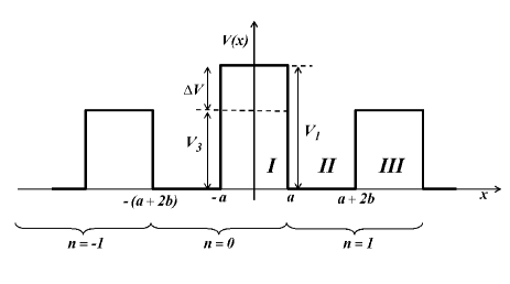
Figure 1: A distorted Kronig-Penney potential. Setting $\Delta V=0$, we obtain a simple Kronig-Penney potential with lattice period $l=2(a+b)$. $n=0,\pm 1,...$ denotes the cell number.

For values of energy $E$ where $|tr(T)|\leq 2$, $t_{\pm}$ are complex numbers of modulus unity:

$$t_{\pm}=e^{\pm ik_{b}l},$$ (18)

and these define the allowed energy bands. For other energies $t_{\pm}$ are real, therefore the solutions are divergent and these define the band gaps. The special cases $t_{\pm}=1$ or $-1$, define the band edges (see the discussion following Eq. (27)). Within the energy bands, Eq. (17) can be rewritten as Bloch wave functions,

$$\psi_{t\pm}(x_{n})=e^{\pm ik_{b}x_{n}}u_{k_{b}}^{\pm}(x_{n}),$$ (19)

where $u_{k_{b}}^{\pm}(x_{n})$ defined as,

$$u_{k_{b}}^{\pm}(x_{n})\equiv e^{\mp ik_{b}(x_{n}-nl)}\left\{\begin{array}[]{cc}A_{0}e^{ik_{2}(x_{n}-nl)}+B_{0}e^{-ik_{2}(x_{n}-nl)}\\ C_{0}e^{ik_{3}(x_{n}-nl)}+D_{0}e^{-ik_{3}(x_{n}-nl)}\end{array},\right.$$ (20)

are the cell periodic functions, which are invariant under any lattice translation. It is obvious from Eq.(19) that $k_{b}$ is the Bloch wave vector.

II.2 Pattern of Parities at the Band Edges

For the particular choice of the position of $x=0$ for setting the symmetry point of the form of the potential, the parity symmetry is manifest. Therefore, all the eigenstates of the Hamiltonian can be chosen to have definite parities. The parity eigenstates can be written as a linear combination of Bloch wave functions:

$$\psi_{p}(x_{n})=A_{p,t+}\psi_{t+}+A_{p,t-}\psi_{t-},$$ (21)

where the subscript $p=\pm 1$ denotes the parity eigenvalue. Writing the wavefunction in the central barrier as,

$$\psi_{p}(x_{0})=e^{ik_{3}x_{0}}+pe^{-ik_{3}x_{0}}\quad{-a\leq x_{0}\leq a},$$ (22)

and matching the wavefunctions at the boundaries $x=\pm a$ the expansion coefficients $A_{p,t\pm}$ are found to be,

$$A_{p,t+}=\frac{A_{0}-p\alpha_{-}{A_{0}}^{\ast}}{\alpha_{+}-\alpha_{-}},$$

$$A_{p,t-}=\frac{A_{0}-p\alpha_{+}{A_{0}}^{\ast}}{\alpha_{-}-\alpha_{+}},$$ (23)

where,

$$A_{0}=\frac{e^{ik_{2}a}}{2}[(1+\frac{k_{3}}{k_{2}})e^{-ik_{3}a}+p(1-\frac{k_{3}}{k_{2}})e^{ik_{3}a}].$$ (24)

(a) Energy bands and parities at their edges

(b) $z_{\pm}$ in the first three energy band in ascending order

Figure 2: (a) The first three energy bands of a KP potential with $a=b=1.5$ and $V_{3}=1$. The pattern of parity signs for this potential is {$+,-,+,-,+,+,-,+,-,-,+,-,+,+,-,+,-,-,+,-,...$}. Note the periodic pattern which is particularly apparent if we disregard the first two signs which belong to the zeroth band. The pattern of periodicity depends on the parameters of the potential. (b) The graphs of $z_{-}$ (solid lines) and $z_{+}$ (dashed lines) for the first three energy bands. Note that these always have values $\pm 1$ at the band edges. Also note that in the third band $z_{\pm}$ change sign by passing through either zero or a divergent point, which changes the sign of parities at all the higher band edges. The particular energy in question is precisely where a resonant state appears.

In the energy bands $\alpha_{\pm}$ can be written as,

$$\alpha_{\pm}=z_{\pm}e^{ik_{2}l},$$ (25)

where the moduli $z_{\pm}$ are given by,

$$z_{\pm}=\frac{0.5\eta\sin(2k_{3}a)}{\cos(2k_{3}a)\sin(2k_{2}b)+\frac{\varepsilon}{2}\sin(2k_{3}a)\cos(2k_{2}b)\mp\sin(k_{b}l)}.$$ (26)

Using Eqs.(25,17) it can be shown that,

$$\psi_{t\pm}(-x)=t_{\pm}z_{\pm}\psi_{t\pm}(x).$$ (27)

At the band edges $|tr(T)|=2$, and since Eq.(16) is true everywhere, we have $t_{+}=t_{-}=1\mbox{ or}-1$. Therefore, Eqs.(14,25) imply $z_{+}=z_{-}=1\mbox{ or}-1$ at the band edges. Consequently the Bloch wave functions at these values of energy become non-degenerate standing waves with definite parity, whose signs are determined by the product of $t_{\pm}$ and $z_{\pm}$, cf. Eq.(27). An alternative reasoning for non-degeneracy of the states at the band edges is the following. At the band edges the Bloch wave vector has modulus $n\pi/l$ and by passing each barrier the wave function is only multiplied by $\pm 1$, consequently the degeneracy of the Bloch wave functions is broken at the band edges and the eigenstates of the Hamiltonian are standing waves with definite parities. These states can be considered as threshold bound states in the absence of any distortion, as a generic feature of any one-dimensional quantum mechanical system. The wave function at the lowest allowed energy has always positive parity. For a periodic potential consisting of delta-functions, the sign of parity alternates at the band edges. However, as we shall discuss, this alternating pattern changes as the barriers are widened. The sign of $t_{\pm}$ at the edge of energy bands alternates for all shapes of potentials but as the width of the barriers grows from zero, the tendency of the wave functions to avoid the barriers and gather in the wells makes $z_{\pm}$ change sign in some energy bands. Therefore, Eq. (27) indicates that the states at the top and bottom of such bands have the same parity. This also leads to a corresponding change in the sign of parities at all higher band edges. The eigenvectors of the transfer matrix at energies where $z_{\pm}$ change sign by passing through either zero or a divergent point, are pure left or right going plane waves. These are called resonant states and are a result of the reflection-less property of the potential at those energies. In Fig. 2, $z_{\pm}$ and the parities at the band edges are shown in the first three energy bands for a particular KP potential. It is interesting that the parities at the band edges and the appearance of resonant states follow some form of periodic pattern, for any choice of the potential parameters, after skipping a few of the lowest lying energy bands. The exact number of bands that needs to be skipped before the periodic structure becomes manifest, and the frequency of the appearance of the resonant states depends more crucially on the width of the barriers. We make the following labeling convention which shall be convenient when we formulate the appropriate forms of the Levinson theorems: The very first gap, the very first energy band, and the very first band edge are labeled as zeroth gap, zeroth band and zeroth band edge, respectively.

III Distorted Kronig-Penney Model

For simplicity we consider a particular distortion of the KP model which is accomplished by only changing the strength of the central barrier to $V_{1}=V_{3}+\Delta V$, as shown in Fig. 1. This breaks the lattice translational symmetry; however, the Hamiltonian is still invariant under the parity operator and the wavefunction in the central barrier can be written as:

$$\psi_{d,p}(x_{0})=e^{ik_{1}x_{0}}+pe^{-ik_{1}x_{0}}\quad{-a\leq x_{0}\leq a},$$ (28)

where the subscript $d$ denotes quantities in the distorted KP model, and $p$ again denotes the parity eigenvalue and

$$k_{1}=\sqrt{\frac{2\mu}{\hbar^{2}}(E-V_{1})}.$$ (29)

From the boundary conditions at $x=\pm a$, the wave functions in the zeroth and first wells are found to be

$$\psi_{d,p}(x_{0}) = A_{d,0}e^{ik_{2}x_{0}}+B_{d,0}e^{-ik_{2}x_{0}},$$ (30)

in the zeroth well

$$\psi_{d,p}(x_{1}) = A_{d,1}e^{ik_{2}(x_{1}-l)}+B_{d,1}e^{-ik_{2}(x_{1}-l)}$$ (31)

in the first well,

where

$$A_{d,1} = \frac{e^{ik_{2}(l-a)}}{2}[(1+\frac{k_{1}}{k_{2}})e^{ik_{1}a}+p(1-\frac{k_{1}}{k_{2}})e^{-ik_{1}a}]$$

$$B_{d,1} = pA^{*}_{d,1},\,B_{d,0}=pA_{d,0}^{*}=pe^{-ik_{2}l}A_{d,1}.$$ (32)

Although the lattice translation symmetry is broken, we can still generate the wave function in the nth well on the right or the left by repeated application of $T$ or $T^{-1}$ on the wave function in the first or the zeroth well, respectively. Therefore, the general wave functions on the right and left sides of the central barrier can be expanded in terms of the eigenstates of the transfer matrix as follows

$$\psi_{l}(x_{n})=A_{l,t+}\psi_{t+}(x_{n})+A_{l,t-}\psi_{t-}(x_{n}),$$

$$n\mbox{\small th well on the left}:\hskip 5.69054ptn=0,\,-1,\,\dots$$ (33)

$$\psi_{r}(x_{n})=A_{r,t+}\psi_{t+}(x_{n})+A_{r,t-}\psi_{t-}(x_{n}),$$

$$n\mbox{\small th well on the right}:\hskip 5.69054ptn=1,\,2,\,\dots.$$ (34)

In general a limited local change in any periodic potential does not change the overall structure of the continua, although one or more states may be displaced below or above the continua, to form localized or bound states in the forbidden energy zones. These bound states appear at the cost of changes in the density of states of the continua Callaway . Since in the forbidden gaps $t_{\pm}$ are real numbers, and Eq. (16) is true everywhere, one of the coefficients $A_{l,t+}$ or $A_{l,t-}$ in Eqs. (33) must vanish for any normalizable solution representing a bound state. A similar statement can be made for the coefficients in Eqs. (34). Hence, due to the parity symmetry, matching the two alternative solutions in the first right well, for example, suffices for obtaining the conditions for the occurrence of bound states:

$$\frac{A_{d,1}}{B_{d,1}}=\alpha_{-}\quad\mbox{if}\quad tr(T)>2,$$ (35)

and

$$\frac{A_{d,1}}{B_{d,1}}=\alpha_{+}\quad\mbox{if}\quad tr(T)<-2.$$ (36)

The energies of the bound states versus $V_{1}$ for the first four energy gaps of a distorted KP potential are plotted in Fig. 3.

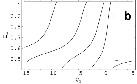
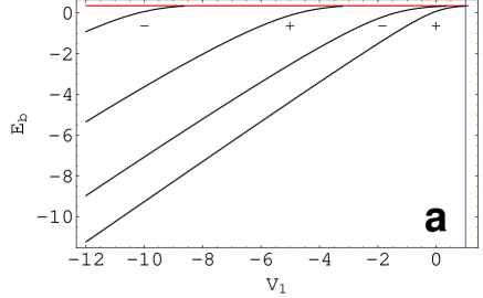
Figure 3: The pattern of bound states which appear due to the presence of a distortion ($\Delta V=V_{1}-V_{3}$), in the first four gaps of a distorted KP potential versus the strength of the central barrier $V_{1}$, depicted in ascending order(a,b,c,d). The particular parameters of the potential are $a=b=1.5$ and $V_{3}=1$. The case $V_{1}=1$ exactly corresponds to the simple KP model. The two bound states for $V_{1}>1$ depicted in the first and third gaps which seem to coincide on the scale shown, are actually similar to the ones depicted in the second gap when exhibited in smaller scale. The energies at the band edges are {0.3355,0.4160,1.0314,1.5405,1.7442,2.8970,3.0840,4.8727}.

Figure 4: The phase shifts in the first four energy bands for the positive and negative parity eigenstates in a distorted KP potential with $a=b=1.5,\,V_{3}=1$ and $V_{1}=-2$, depicted in ascending order (a,b,c,d). Note that the phase shifts have values which are integer multiple of $\pi/2$ at the band edges.

Now we can discuss the phase shifts within the allowed energy bands. In the bands both $\psi_{t+}(x_{n})$ and $\psi_{t-}(x_{n})$ are allowed and the expansion coefficients in Eqs. (33) and  (34) are found by matching the two alternative solutions in the wells adjacent to the central barrier, as before,

$$\begin{array}[]{ll}A_{l,t+}=\frac{A_{d,0}-p\alpha_{-}A^{*}_{d,0}}{\alpha_{+}-\alpha_{-}},\quad A_{r,t+}=\frac{A_{d,1}-p\alpha_{-}A^{*}_{d,1}}{\alpha_{+}-\alpha_{-}}t_{-}\end{array}$$ (37)

$$\begin{array}[]{ll}A_{l,t-}=\frac{A_{d,0}-p\alpha_{+}A^{*}_{d,0}}{\alpha_{-}-\alpha_{+}},\quad A_{r,t-}=\frac{A_{d,1}-p\alpha_{+}A^{*}_{d,1}}{\alpha_{-}-\alpha_{+}}t_{+}\end{array}$$ (38)

Substituting $\psi_{t+}(x_{n})$ and $\psi_{t-}(x_{n})$ from Eq. (19) in Eqs. (33) and  (34), the scattering states in the bands can be rewritten as:

$$\psi_{p,l}(x_{n}) = A_{l,t+}u_{k_{b}}^{+}(x_{n})e^{ik_{b}x_{n}}+A_{l,t-}u_{k_{b}}^{-}(x_{n})e^{-ik_{b}x_{n}},$$ (39)

$$\mbox{\small nth well on the left}:\hskip 5.69054ptn=0,\,-1,\,...$$

$$\psi_{p,r}(x_{n}) = A_{r,t+}u_{k_{b}}^{+}(x_{n})e^{ik_{b}x_{n}}+A_{r,t-}u_{k_{b}}^{-}(x_{n})e^{-ik_{b}x_{n}},$$ (40)

$$\mbox{\small nth well on the right}:\hskip 5.69054ptn=1,\,2,\,...$$

Now for each parity state the phase shift, $\delta_{p}(E,V_{1})$, is obtained by comparing the coefficients of $e^{ik_{b}x_{n}}$ on the left and right-hand sides:

$$e^{2i\delta_{p}(E,V_{1})}=\frac{A_{d,1}-p\alpha_{-}A^{*}_{d,1}}{A_{d,0}-p\alpha_{-}A_{d,0}^{*}}t_{-}.$$ (41)

As the distortion is turned off, the bound states merge into the bands and the phase shifts vanish, and this alleviates the inherent ambiguity of the phase shifts by integer multiples of $\pi$. On the band edges where $\alpha_{+}=\alpha_{-}$ it can be easily shown that,

$$e^{2i\delta_{p}(E,V_{1})}=\pm 1,$$ (42)

which means the phase shifts are integer multiples of $\frac{\pi}{2}$ at each band edge.

For simplicity, we consider a particular distortion and compute the phase shifts of the parity eigenstates in the first four energy bands of a distorted KP potential for $V_{1}=-2$ and plot the results in Fig. 4. We base our conclusions on this set of parameters. However, we have checked the validity of our forthcoming conclusions for a wide range of parameters including changing the strength of the central barrier and the widths $a$ and $b$. Considering the historical background and the explanation given in the introduction about the different contributions of half bound states, one might expect that for a given band, the difference between the phase shifts at the two band edges to count the number of states which emerge out of that band minus the number that enter that band, with the proper account of the threshold bound states. Moreover, the strong form of the Levinson theorem for an isolated potential states that the value of the phase shift at the edge of the continuum is equal to the total number of bound states that have exited minus the ones that have entered the continuum from that edge, as the distortion is formed. However, as we shall see, these are not quite true in the case of periodic potentials with isolated distortions, and need one additional modification.

We now set out to extract the strong form of the Levinson theorem from our results. Let us start with the zeroth energy band. As shown in Fig. 3 (a), at zero strength of the distortion, i.e. $V_{1}-V_{3}=\Delta V=0$, there is one positive parity threshold bound state at the lower edge of the zeroth energy band which is pulled down into the zeroth energy gap as $V_{1}$ is decreased. Reducing the value of $V_{1}$ from $1$ to $-2$, a second bound state with negative parity also emerges from this edge. Therefore, the expected values for the phase shifts of positive and negative parity eigenstates at this edge are $\frac{\pi}{2}$ and $\pi$, respectively. The statement derived in stronglev0 ; stronglev1 is that these phase shifts directly count the number of bound states that emerge out of the band edge under consideration as the strength of the potential is changed. For the aforementioned positive parity bound state, it was already a threshold state at zero distortion and its emergence as a complete bound states counts as one half. These values are in agreement with phase shift diagrams in Fig. 4(a). At the upper edge of the zeroth energy band, Fig. 3 (b), there is a negative parity threshold bound state at zero distortion, which sinks into the band as $V_{1}$ is reduced to $-2$. Thus the phase shifts at this edge are expected to be zero and $-\frac{\pi}{2}$ for positive and negative parity eigenstates, respectively. However, the phase shift values at this edge, as shown in Fig. 4 (a), differ by a minus sign from what is speculated.

At the lower edge of the first energy band, there is a positive parity threshold bound state at zero strength of the distortion, which is pulled down to the first energy gap as the value of $V_{1}$ is reduced from $1$, Fig.3 (b). Later a negative parity bound state emerges from this edge when $V_{1}$ is reduced further towards $-2$. The expected phase shift values for positive and negative eigenstates at this edge are $\frac{\pi}{2}$ and $\pi$, respectively, which again differ by a minus sign from the actual phase shift values at this edge, as shown in Fig.4 (b).

Comparison between the phase shifts of eigenstates in higher energy bands and the number of bound states displaced out of or into these bands mandate a different rule for the strong form of the Levinson theorem for periodic potentials, which is

$$\delta_{\pm}(E_{s},V_{1})=(-1)^{s}(N_{exit}^{s,\pm}-N_{enter}^{s,\pm})\pi,$$ (43)

where $s$ is the energy gap index, $E_{s}$ labels the energy value at either the lower or upper boundary of the $s$th gap, and $N_{exit}^{s,\pm}$ and $N_{enter}^{s,\pm}$ are the total number of bound states of definite parity that exit or enter the energy bands from that particular boundary. Any threshold bound state involved in this process counts as one half, as explained in the introduction, cf. Eqs.(4,I) and their following explanations. Subtracting the expression for the phase shifts at the lower and upper edges of the $s$th energy band, the Levinson theorem is easily obtained,

$$\Delta\delta_{s,\pm} \equiv \delta_{\pm}(E_{s}^{l},V_{1})-\delta_{\pm}(E_{s}^{u},V_{1})$$ (44)

$$= \pi(-1)^{s}(N_{out}^{s,\pm}-N_{in}^{s,\pm})=\pi(-1)^{s}\mathcal{D}_{s,\pm},$$

where $s$ is the energy band index, $\delta_{\pm}(E_{s}^{l},V_{1})$ and $\delta_{\pm}(E_{s}^{u},V_{1})$ are the phase shifts of eigenstates of definite parity at the lower and upper boundaries of the $s$th energy band. $N_{out}^{\pm,s}$ and $N_{in}^{s,\pm}$ denote the number of bound states that leave or enter the $s$th band as the distortion is turned on. Threshold bound states count as one half, exactly as explained before. The quantity $\mathcal{D}_{s,\pm}$ denotes the spectral deficiency in the $s$th band, for each parity separately. This formula can be easily cast into the form of Eq. (I). Therefore, the only difference between both forms of the Levinson theorem for the distorted KP potential and their forms for isolated potentials in relativistic stronglev0 ; stronglev1 or non-relativistic quantum mechanics is the factor $(-1)^{s}$. By adding the phase shifts at the lower and upper boundaries of the $s$th gap, we can also present the following interesting relationship between that quantity and the number of bound states present in that gap due to the distortion, $N_{s,\pm}$,

$$\delta_{\pm}(E_{s}^{l},V_{1})+\delta_{\pm}(E_{s}^{u},V_{1})=\pi(-1)^{s}N_{s,\pm}.$$ (45)

We can combine Eqs. (44,45) to relate the total number of bound states, deficiencies, and the phase shifts

$$\delta_{\pm}(E_{0},V_{1}) - \delta_{\pm}(E_{1},V_{1})-\delta_{\pm}(E_{2},V_{1})+$$ (46)

$$\delta_{\pm}(E_{3},V_{1}) + \delta_{\pm}(E_{4},V_{1})+\dots=\pi\Sigma N_{s,\pm}=\pi\Sigma\mathcal{D}_{s,\pm},$$

where the energies of the boundaries are labeled consecutively for clarity. This equation makes the completeness relationship manifest. For the special case of the zeroth gap and band edge Eq. (45) reduces to,

$$\delta_{\pm}(E_{0},V_{1}))=\pi N_{0,\pm},$$ (47)

which is what we expect from Eq. (43).

IV Conclusions

In this paper we calculated the band structure, continuum states and their phase shifts, and the bound states for a distorted KP model. We obtain the strong form of the Levinson theorem as stated in Eq.(43) which relates the phase shifts at each band edge to the number of states that cross that edge. Obviously threshold bound states count as one half as explained in the text. From this theorem we can easily conclude the Levinson theorem as stated in Eq.(44), which relates the difference between the phase shifts at edges of a given band to the spectral deficiency of that band. Both theorems are identical to their counterparts for localized potentials in relativistic and non-relativistic quantum mechanics, except for a factor of $(-1)^{s}$, where $s$ denotes the adjacent gap or the band index, for the strong or weak form of the theorem, respectively. We have also obtained a relationship between the phase shifts at the edges of any gap to the number of bound states present in that gap Eq.(45), and an overall relationship exhibiting completeness of the spectrum Eq.(46).

Acknowledgements

We would like to thank the research office of the Shahid Beheshti University for financial support.

References

- (1) L. Esaki, R. Tsu, Appl. Phys. Lett. 22 (1973) 562.
- (2) C. Rorres, J. Appl. Math. 27 (1974) 303 SIA.
- (3) D. Kiang, Am. J. Phys. 42 (1974) 785.
- (4) P. Erdös, R. C. Herndon, Adv. Phys. 31 (1982) 65.
- (5) D.J. Vezzetti, M. Cahay, J. Phys. D. 19 (1986) L53.
- (6) H-W Lee, A. Zysnarski, P. Kerr, Am. J. Phys. 57 729 (1989).
- (7) H. Yamamoto, M. Arakawa, K. Taniguchi Appl. Phys. A 50 (1990) 577.
- (8) T.M. Kalotas, A.R. Lee Eur. J. Phys. 12 (1991) 275.
- (9) D.J. Griffiths, N.F. Taussig, Am. J. Phys. 60 (1992) 883.
- (10) D.W. L. Sprung, Hua Wu, J. Martorell, Am. J. Phys. 61 (1993) 1118.
- (11) M.G. Rozman, P. Reineker, R. Tehver, Phys. Rev. A 49 (1994)3310.
- (12) C.L. Roy, A. Khan, Phys. Status Solidi B 176 (1993) 101.
- (13) P. Erdös, R.C. Herndon, Solid State Commun. 98 (1996) 495.
- (14) M.G. Rozman, P. Reineker, R. Tehver, Phys. lett. A 187 (1994) 127.
- (15) D. Bar, L.P. Horwitz, Eur. Phys. J. B. 25 (2002) 505.
- (16) P. Pereyra, E. Castillo, Phys. Rev. B. 65 (2002) 205120.
- (17) A. Peres, J. Math. Phys. 24 (1983) 1110.
- (18) P. Erdös, E Livitti, R.C. Herndon, J. Phys. D 30 (1997) 338.
- (19) M.S. Marinovyz, Bilha Segevy, J. Phys. A 29 (1996) 2839.
- (20) F. Barra, P. Gaspard, J. Phys. A 32 (1999) 3357.
- (21) J.J. Rehr, W. Kohn, Phys. Rev. B 9 (1973) 1981.
- (22) Y. Takagaki, D.K. Ferry, Phys. Rev. B 45 (1992) 6715.
- (23) Wei-Dong Sheng, Jian-Bai Xia, J. Phys.: Condens. Matter 8 (1996) 3635.
- (24) D.W. Sprung, J.D. Sigetich, Hua Wu, J. Martorell, Am. J. Phys. 62 (2000) 2458.
- (25) T. Kostyrko, Phys. Rev. B 62 (2000) 2458.
- (26) D.J. Fernandez, C.B. Mielnik, O. Rosas-Ortiz, B.F. Samsonov, J. Phys. A: Gen. 35 (2002) 4279.
- (27) M. Sassoli de Bianchi, J. Math. Phys. 35 (1994) 2719.
- (28) M. Sassoli de Bianchi, M. Di Ventra, J. Math. Phys. 36 (1994) 1753.
- (29) T. Aktosun, M. Klaus, C. van der Mee, J. Math. Phys. 39 (1998) 4249.
- (30) P. Garpena, V. Gasparian, M. Ortuno, Eur. Phys. J. B 8 (1999) 635.
- (31) T. Aktosun, J. Math. Phys. 40 5289 (1999).
- (32) N. Levinson, K. Dan. Vidensk. Selsk. Mat. Fys. Medd. 25 (1949) 9.
- (33) J.M. Jauch, Helv. Phys. Acta 30 (1957) 143.
- (34) R.G. Newton, J. Math. Phys. 1 (1960) 319.
- (35) R.G. Newton, Ann. Phys. (NY) 194 (1989) 173.
- (36) Z.Q. Ma, J. Phys. A 39 (2006) R659.
- (37) L.J. Boya, J. Casahorrán, Int. J. Theo. Phys. 46 (2007) 1998.
- (38) S.S. Gousheh, Quantum numbers of solitons Ph.D. Desertation, Texas U. UMI-94-00894, 139pp, Aug. 1993.
- (39) S.S. Gousheh, Phys. Rev. A 65 (2002) 032719.
- (40) S.S. Gousheh, Nucl. Phys. B 428 (1994) 189.
- (41) A. Calogeracos, N. Dombey, Phys. Rev. Lett. 93 (2004) 180405.
- (42) Zhong-Qi Ma, Shi-Hai Dong, Lu-Ya Wang, Phys. Rev. A 74 (2006) 012712.
- (43) J. Callaway, Phys. Rev. 154 (1967) 515.
- (44) P. Senn, Am. J. Phys. 56 (1988) 916.
- (45) G. Barton, J. Phys. A: Math. Gen. 18 (1985) 479.
- (46) W. van Dijk, K.A. Kiers, Am. J. Phys. 60 (1992) 520.
- (47) Y. Nogami, C.K. Ross, Am. J. Phys. 64 (1996) 923.
- (48) K.A. Kiers, W. van Dijk, J. Math. Phys. 37 (1996) 6033.
- (49) V.E. Barlette, M.M. Leite, S.K. Adhikari, Eur. J. Phys. 21 (2000) 435.
- (50) R. de L. Kronig, W.J. Penney, Proc. R. Soc. London, Ser. A 130 (1930) 499.
- (51) J.P. McKelvey, Solid State and Semiconductor Physics, Harper & Row, New York, 1966.
- (52) D. Mukherji, B.R. Nag, Phys. Rev. B 12 (1975) 4338.
- (53) G. Bastard, Phys. Rev. B 24 (1981) 5693.
- (54) J.N. Schulman, Y.C. Chang, Phys. Rev. B 24 (1981) 4445.
- (55) B.A. Vojak, W.D. Laiding, N. Holonyak Jr., M.D. Caramas, J.J. Coleman, P.D. Dapkus, J. Appl. Phys. 52 (1981) 621.
- (56) G. Bastard, Phys. Rev. B 25 (1982) 7584.
- (57) K. Seeger, Semiconductor Physics, 3rd ed., Springer Berlin, 1985.
- (58) Hung-Sik Cho, P.R. Pruncnal, Phys. Rev. B 36 (1987) 3237.
- (59) Shao-Hua Pan, Si-min Feng, Phys. Rev. B 44 (1991) 5668.
- (60) F. Szmulowicz, Eur. J. Phys. 18 (1997) 392.
- (61) F. Maiz, A. Hfaiedh, N. Yacoubi, J. Appl. Phys. 83 (1998) 867.
- (62) Szu-Ju Li, Chi-Hon Ho, Yao-Tsung Tsai, Int. J. Numer. Model 20 (2007) 109.
- (63) X-H Wang, B-Y Gu, G-Z Yang, J. Wang, Phys. Rev. B 58 (1998) 4629.
- (64) D.W.L. Sprung, J. Sigetich, P. Jagiello, J. Martorell, Phys. Rev. B 67 (2003) 085318.
- (65) T.A. Weber, Solid State Comm. 90 (1994) 713.
- (66) T.A. Weber, D.L. Pursey, Phys. Rev. A 57 (1998) 3534.
- (67) E. Merzbacher, Quantum Mechanics, 3rd ed., John Wiley & Sons, Inc. 1998.