Dirichlet Casimir Energy for a Scalar Field in a Sphere: An Alternative Method

Abstract

In this paper we compute the leading order of the Casimir energy for a free massless scalar field confined in a sphere in three spatial dimensions, with the Dirichlet boundary condition. When one tabulates all of the reported values of the Casimir energies for two closed geometries, cubical and spherical, in different space-time dimensions and with different boundary conditions, one observes a complicated pattern of signs. This pattern shows that the Casimir energy depends crucially on the details of the geometry, the number of the spatial dimensions, and the boundary conditions. The dependence of the sign of the Casimir energy on the details of the geometry, for a fixed spatial dimensions and boundary conditions has been a surprise to us and this is our main motivation for doing the calculations presented in this paper. Moreover, all of the calculations for spherical geometries include the use of numerical methods combined with intricate analytic continuations to handle many different sorts of divergences which naturally appear in this category of problems. The presence of divergences is always a source of concern about the accuracy of the numerical results. Our approach also includes numerical methods, and is based on Boyer’s method for calculating the electromagnetic Casimir energy in a perfectly conducting sphere. This method, however, requires the least amount of analytic continuations. The value that we obtain confirms the previously established result.

1 Introduction

The Casimir effect is one of the most interesting manifestations of the nontrivial structure of the vacuum state in quantum field theory. This effect appears when nontrivial boundary conditions or background fields are present (e.g. solitons). In 1948 Casimir predicted the existence of this effect as an attractive force between two infinite parallel uncharged perfectly conducting plates in vacuum [1, 2] (for a general review on the Casimir effect, see Refs. [3, 4, 5, 6, 7]). This effect was subsequently observed experimentally by Sparnaay in 1958 [8]. Up to now, most experiments on the measurement of the Casimir forces have been performed with parallel plates [9] or with a sphere in front of a plane [10, 11, 12, 13]. Furthermore, the configuration of two eccentric cylinders have both experimental and theoretical interest [14]. The majority of the investigations related to the Casimir effect concern the calculation of this energy or the resulting forces for different fields in different geometries with different boundary conditions imposed [15]. These cases include parallel plates [1, 2], cubes [16, 17, 18, 19, 20, 21], cylinders [22, 23, 24, 25, 26, 27, 28, 29], and spherical geometries [15, 30, 31, 32]. This effect has even been investigated in connection with the properties of the space-time with extra dimensions [7, 33, 34], and nowadays it is known that the Casimir energy depends strongly on the geometry of the space-time and on the boundary conditions imposed [35, 36]. In fact, an interesting question is the determination of the conditions under which the forces acting on the boundaries for closed geometries are attractive or repulsive in arbitrary spatial dimensions [37, 38, 39, 40, 41, 42].

The Casimir effect has many applications in different branches of physics. Perhaps the first extensive study of the Casimir effect was in Particle Physics and in connection with the development of the bag model of hadrons [6, 30, 43, 44, 45, 46, 47, 48, 49]. One of the most fascinating and open problems of theoretical physics is the cosmological constant [50, 51, 52, 53, 54]. This constant is also a candidate for the dark energy [51, 53, 55], and the Casimir energy has been studied in this connection [51, 53, 56]. Moreover, the presence of the Casimir forces in many different phenomena of condensed matter and laser physics have been established both theoretically and experimentally [57, 58, 59, 60]. In particular, the study of the Casimir effect for massless scalar fields is not only of theoretical interest but also has direct relevance to physical systems such as Bose-Einstein condensates [61, 62, 63].

Calculations of the Casimir energy in spherically symmetric configurations have attracted the interest of physicists for many years [30, 31, 32, 45, 46, 47, 48, 49]. As Boyer [64] first showed, the Casimir pressure exerted by the electromagnetic (EM) field on the walls of a perfectly conducting spherical vessel is repulsive (see also [65]). The reported Casimir energy and pressure of a scalar field confined in a spherical vessel with Dirichlet boundary condition is also reported to be positive [66, 67, 68, 69, 70, 71]. Comparison between the reported values of the Casimir energy for closed geometries show that these values depend crucially on three major factors: first the details of the geometries (e.g. spheres or cubes), second the number of space dimensions, and third the boundary conditions. To be very concrete we have collected all of the reported results for various cases and display them in Table (1). We should mention that all of the results obtained for cubical geometry are exact, while the ones for spherical geometries are obtained approximately by various numerical methods.

Dimension	Field	B.C.s	Cube	Sphere
2	Scalar	$\mathcal{D}$	+0.041	+0.000672-0.003906/s
2	Scalar	$\mathcal{N}$	-0.22	-0.183123-0.019531/s
2	EM	Conductor	-0.22	-0.183123-0.019531/s
3	Scalar	$\mathcal{D}$	-0.016	+0.002819
3	Scalar	$\mathcal{N}$	-0.29	-0.223458
3	EM	Conductor	+0.092	+0.046200
4	Scalar	$\mathcal{D}$	+0.0061	-0.000655+0.000267/s
4	Scalar	$\mathcal{N}$	-0.33	-0.260872-0.044716/s
4	EM	Conductor	-0.044	-0.197834-0.033768/s
5	Scalar	$\mathcal{D}$	-0.0025	-0.000288
5	Scalar	$\mathcal{N}$	-0.37	-0.270281
5	EM	Conductor	+0.021	-0.006362

Table 1: The Casimir energies for the EM field (with boundary condition consistent with a perfectly conducting cavity denoted by “Conductor”) and massless scalar fields (with Dirichlet and Neumann boundary conditions denoted by “$\mathcal{D}$” and “$\mathcal{N}$”, respectively). The values are displayed for the space dimensions $D=\{2,3,4,5\}$, for cubical and spherical geometries. The quantity $s$ is a regularization factor which should be taken to zero. The values are displayed for a cube with unit volume and a sphere with radius $a=1$, all in units $\hbar c=1$.

As one can see from the Table (1), for the spherical cases in even spatial dimensions, there always remains an unresolved divergent factor. For the case of massless scalar fields with the Neumann boundary condition, the Casimir energy is always negative regardless of the details of the geometry and the number of space dimensions. Therefore, one might conclude that there are no surprises there. However, for the case of massless scalar fields with Dirichlet boundary conditions there is a sign factor $(-1)^{D}$ for the case of cubes [72], and $(-1)^{\mbox{\footnotesize{Floor}}(D/2-1)}$ for the case of spheres [69], where $D$ denotes the number of space dimensions. For the case of EM field inside a perfectly conductor there is a sign factor $(-1)^{D+1}$ for the case of cube, and no obvious sign factor for the case of sphere.

Now we concentrate on the case of three spatial dimensions. At a first glance, the reported results for the case of a massless scalar field confined in a spherical geometry with Dirichlet boundary condition seem anomalous because it is the only case for which the two geometries do not have the same sign of the Casimir energy, and this has caused a controversy in the literature. As far as this controversy is concerned, L.A. Manzoni and W.F. Wreszinski [73], try to justify these results by showing that the Casimir forces in both cases are repulsive. It has been claimed that for the EM case, the deformation of a spherical shell of radius $a$ into a cubical shell of length $L$ with $L\approx 2a$, should not change the sign and approximately the magnitude of the Casimir energy, when the boundary conditions are unchanged [21, 74, 75]. We believe that their claim is reasonable. However, it is inconsistent with the results for the EM field in five spatial dimensions and the massless scalar field with Dirichlet boundary conditions in three and four spatial dimensions. Therefore, it is worth studying this problem in more details, and here we concentrate on the three dimensional case.

Although, the Casimir energy for the case of the cube is exactly solvable [74], the presence of divergences inherent in these sorts of problems require regularization and analytic continuation methods [76], and this has been a source of criticism for this calculation [77, 78]. Since the Casimir energy for the case of the sphere is not exactly solvable, it requires the utilization of numerical methods. The use of numerical methods for problems which include divergences could be a source of even greater concerns about the accuracy of the final results. When the problem is plagued with multitude of divergences, the numerical methods should include delicate and carefully planed regularization and possibly analytical continuation techniques. The problem addressed in this paper is in this category, and we calculate this case using an alternative method which requires the least amount of regularization and analytic continuation schemes.

There are three general methods for calculating the Casimir energy for the spherical case, which as mentioned earlier all include numerical parts. The first method is the Green function formalism [32]. In this method one encounters an infinite sum of integrals over the modified Bessel functions. It can be shown that each of the integrals converges and the sum can be calculated numerically by using the asymptotic behavior of the modified Bessel functions for all real D. The plot of the Casimir pressure as a function of continuously variable D show that the result is infinite for even dimensions [32]. The second method is the zeta function technique. For example, G. Cognola et al [69] use the zeta function technique to obtain the Casimir energies for spherical symmetric cavities, for different boundary conditions, and fields in D space dimensions. The third method is the direct mode summation using contour integration [70]. This method is based on the direct summation of the frequencies and the main tool employed is the Cauchy theorem. This employment lets the authors sum the zeros of the Bessel functions more easily.

The method we use in this paper is based on the Boyer’s method which was used for the EM field in a sphere. An important part of the Boyer’s method is to confine the system inside a similarly shaped but larger shell, and then to subtract the energies of two configurations with the same size outer shells and different size inner shells. In this subtraction scheme, most of the infinities automatically cancel without any need to use analytic continuations. As a matter of fact in this method, the Casimir energy is simply the work done on the system in deforming the initial configuration to the one under consideration. Therefore, the quantity just defined has an obvious physical interpretation. One can then let the radii of the outer shells and the second inner shell go to infinity. We shall henceforth refer to this subtraction scheme as the Boyer Subtraction Scheme (BSS). We recently used this method to directly compute the lowest order Casimir energy for the EM field inside a rectangular waveguide Ref. [79], and the lowest order radiative corrections for the Casimir energy for a scalar field for the parallel plate problem in various space-time dimensions  [80, 81].

In this paper we use BSS for a massless scalar field confined in a sphere with the Dirichlet boundary condition. The analytic part of our calculation is analogous to the one used by Boyer for the TE modes, and is done in section 2. In section 3, we present the final part of our calculations which, similar to the Boyer’s paper, is numerical. However, our numerical calculations differ from that paper. We introduce a method to extrapolate the sum of all the zero point energies for a given value of the angular momentum $\ell$. In order to proceed with the summation over $\ell$, we first introduce a second extrapolation method to obtain the optimal form of the summand. We then sum over all $\ell$ by using the zeta function analytic continuation technique to remove the infinities and extract the finite part. Our final result agrees with the established value obtained in [66, 67, 68, 70, 71]. In section 4, we summarize and discuss our results.

2 Analytic Part of the Calculation of Casimir Energy in a Sphere

In this section we setup all the physical and mathematical machinery for the calculation of the Casimir energy for a real massless scalar field with Dirichlet boundary condition for a spherical geometry. The mathematical part introduced in this section parallels closely the one due to Boyer [64] for the computation of the Casimir energy for the EM field inside a perfectly conducting sphere. The similarity between our calculation and that of Boyer stems from the fact that the expressions for the Casimir energy for the TE mode of the EM field is similar to the massless scalar field with Dirichlet boundary condition [6]. The important difference is that the term with $\ell=0$ is allowed in the latter case. Moreover, there is no analogue of the TM mode in our problem due to choice of boundary condition. As we shall see, this forces us to encounter some new divergences. A close examination of Boyer’s work show that when both modes are present these divergences cancel. The final expression obtained in this section cannot be solved analytically, and we solve it numerically in the next section.

The Casimir energy is defined as the difference between the sum of the zero point energies of all the modes in the bounded region considered, and the free case. In order to find all of the modes inside a sphere we have to solve the Klein-Gordon equation for a massless scalar field, with the appropriate boundary condition. Due to spherical symmetry, each energy level $E_{\ell}$ will be $(2\ell+1)$ fold degenerate. Therefore we have the following expression for the total zero point energy,

$$E=\sum\limits_{\ell=0}^{\infty}\left(2\ell+1\right)\sum\limits_{s=1}^{\infty}\frac{\hbar\omega_{\ell,s}}{2}=\frac{\hbar c}{2}\sum\limits_{\ell=0}^{\infty}\left(2\ell+1\right)\sum\limits_{s=1}^{\infty}k_{\ell,s},$$ (1)

where $\omega_{\ell,s}$ and $k_{\ell,s}$ are the normal modes frequencies and wave-vectors, respectively, and the index $s$ refers to the root number for a given value of $\ell$. Since there are an infinite number of normal modes of increasingly high frequency, this energy is infinite, as usual. However, as mentioned before $E_{\mbox{\footnotesize Cas.}}$ is obtained by the subtraction of this zero-point energy from the analogous one for the free case. An essential part of the Boyer’s method is to enclose this sphere inside a larger one. Then a similar configuration is considered but with a different radius for the inner sphere (see Fig. (1)). Then the zero point energies of these two configurations are subtracted from each other, and many of the infinities cancel each other out. Then the radii of all the spheres except the original inner sphere (the one with radius ‘$a$’) is taken to infinity.

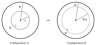
Figure 1: Left figure shows two concentric spheres with radii $a$ and $R$ (configuration ‘A’). The right figure shows a similar configuration with different radius for the inner sphere (configuration ‘B’). To calculate the Casimir energy, the zero point energies of these two spherical configurations are to be subtracted according to the Eq. (2). The label ‘I’ refers to the inner sphere and ‘II’ the outer annular region. In the final step, $R\to\infty$, while $\eta$ is kept fixed.

Therefore our expression for the Casimir energy is given in Eq. (2),

$$E_{\mbox{\footnotesize Cas.}}=\lim_{R\to\infty}\left[(E^{A}_{I}+E^{A}_{II})-(E^{B}_{I}+E^{B}_{II})\right].$$ (2)

Using Eqs. (1,2) we have,

$$\small{E_{\mbox{\footnotesize Cas.}}}=\small{\lim\limits_{R\to\infty}\lim\limits_{\lambda\to 0}\frac{\hbar c}{2}\sum\limits_{\ell=0}^{\infty}\left(2\ell+1\right)}$$ (3)

$$\times\Bigg{[}\sum\limits_{s=1}^{\infty}k_{\ell,s}\left(a\right)\,g\left(\lambda k_{\ell,s}\left(a\right)\right)+\sum\limits_{S=1}^{\infty}K_{\ell,S}\left(a,R\right)\,g\left(\lambda K_{\ell,S}\left(a,R\right)\right)-\{a\to R/\eta\}\Bigg{]},$$

where $k_{\ell,s}(a)$ and $K_{\ell,S}\left(a,R\right)$ are the wave-vectors for the inner sphere and annular region, respectively, and $g(\lambda k_{\ell,s}(a))=e^{-\lambda k_{\ell,s}\left(a\right)}$ is a convergence factor which eventually goes to one as $\lambda\to 0$. Moreover the index $S$ is defined analogously to $s$, but for the annular region.

The imposition of the boundary condition is explained in A, where the relationships between the root indices, $s$ and $S$, and the wave-vectors $k_{\ell,s}\left(a\right)$ and $K_{\ell,S}\left(a,R\right)$, are obtained. Using the results obtained in A and the Euler-Maclaurin Summation Formula (EMSF), we calculate the limit $R\to\infty$ of terms in Eq. (3) coming from the annular regions in B. There we show how in this limit, most of the infinities coming from these regions cancel due to BSS, and all of the remaining finite terms approach zero. The final result is that the two indicated sums turn into integrals with no remainder. As explained below in more details, the two integrals eventually cancel the infinities coming from their respective inner spheres, and their residual infinities cancel each other. We finally obtain,

$$\vspace{-0.4cm}E_{\mbox{\footnotesize Cas.}}=\mathop{\lim}\limits_{R\to\infty}\mathop{\lim}\limits_{\lambda\to 0}\frac{\hbar c}{2}\sum\limits_{\ell=0}^{\infty}(2\ell+1)\Bigg{[}\sum\limits_{s=1}^{\infty}k_{\ell,s}(a)g(\lambda k_{\ell,s}(a))$$

$$\hskip 93.89418pt+\int_{S=1}^{\infty}dS\,K_{\ell,S}(a,R)g(\lambda K_{\ell,S}(a,R))-\{a\rightarrow R/\eta\}\Bigg{]},$$ (4)

where the continuous variable $S$ is associated with the discrete root number $S_{\ell}(a,K)$ and appears when we use EMSF. The above equation is similar to the expression obtained by Boyer for the TE mode, with the only difference being the inclusion of $\ell=0$ in this case. It is obvious from their definitions that $K_{\ell,S}(a)$ and $S_{\ell}(a,K)$ are in one to one correspondence. Therefore we can change the variable of integration from $S$ to the continuous version of the wave-vectors, which we shall denote by $K$ for brevity of notation, and using Eq. (A.10) we have,

$$\vspace{-0.3cm}E_{\mbox{\footnotesize Cas.}}=\small{\mathop{\lim}\limits_{R\to\infty}\mathop{\lim}\limits_{\lambda\to 0}\frac{\hbar c}{2}\sum\limits_{\ell=0}^{\infty}(2\ell+1)\Bigg{[}\sum\limits_{s=1}^{\infty}k_{\ell,s}(a)g(\lambda k_{\ell,s}(a))-\displaystyle\int_{K=K_{\ell,1}(a,R)}^{\infty}dK\,\frac{ds_{\ell}(a,K)}{dK}K\,g(\lambda K)}$$

$$\hskip 91.04872pt+\int_{K=K_{\ell,1}(a,R)}^{\infty}dK\,\frac{ds_{\ell}(R,K)}{dK}K\,g(\lambda K)-\{a\rightarrow R/\eta\}\Bigg{]}.\hskip 11.38092pt$$ (5)

Rewriting Eq. (2) and rearranging terms we have,

$$E_{\mbox{\footnotesize Cas.}}=\mathop{\lim}\limits_{R\to\infty}\mathop{\lim}\limits_{\lambda\to 0}\frac{\hbar c}{2}\sum\limits_{\ell=0}^{\infty}(2\ell+1)\Bigg{\{}\Bigg{[}\sum\limits_{s=1}^{\infty}k_{\ell,s}(a)g(\lambda k_{\ell,s}(a))-\int_{K=K_{\ell,1}(a,R)}^{\infty}dK\,\frac{ds_{\ell}(a,K)}{dK}K\,g(\lambda K)$$

$$\hskip 31.2982pt\hskip 56.9055pt-\{a\rightarrow R/\eta\}\Bigg{]}-\int_{K=K_{\ell,1}(R/\eta,R)}^{K=K_{\ell,1}(a,R)}dK\frac{ds_{\ell}(R,K)}{dK}K\,g(\lambda K)\Bigg{\}}.$$ (6)

As shown in B, Eqs. (B.8,B.9), in the limit $R\to\infty$, the wave-vectors $K_{\ell,1}(a,R)$ and $K_{\ell,1}(R/\eta,R)$ not only decrease exponentially in $\ell$, but also go to zero as $1/R$. So, the difference between the upper and lower limits of the last integral approaches zero and since the integrand is not singular, there is no contribution coming from this term to $E_{\mbox{\footnotesize Cas.}}$. Also, the lower limits of the remaining integrals can be extended to $\small{K=0}$.

We can use the simplest form of the EMSF to make the first term in Eq. (2) more amenable to computation,

$$\sum\limits_{s=1}^{\infty}k_{\ell,s}(a)g(\lambda k_{\ell,s}(a))=\int_{s=1}^{\infty}ds\,k_{\ell,s}(a)\,g(\lambda k_{\ell,s}(a))+\frac{1}{2}[k_{\ell,1}(a)g(\lambda k_{\ell,1}(a))]$$

$$\hskip 42.67912pt+\int_{s=1}^{\infty}ds\Big{(}s-[s]-\frac{1}{2}\Big{)}\frac{d}{ds}[k_{\ell,s}(a)\,g(\lambda k_{\ell,s}(a))],$$ (7)

where $[s_{\ell}(a,k)]$ denotes the Floor Function. The one to one correspondence of $s_{\ell}(a,k)$ and $k_{\ell}(a,s)$ is analogous to the previous case which was for the annular regions. Therefore, we can again change the variable of the integration from $s$ to $k$, and by adding and subtracting appropriate terms we can extend all of the lower limits of the integrals to zero. We obtain:

$$\sum\limits_{s=1}^{\infty}k_{\ell,s}(a)g(\lambda k_{\ell,s}(a))=\int_{k=0}^{\infty}dk\frac{ds_{\ell}(a,k)}{dk}\,k\,g(\lambda k)-\int_{k=0}^{k=k_{\ell,1}(a)}dk\frac{ds_{\ell}(a,k)}{dk}\,k\,g(\lambda k)$$

$$\hskip 51.21504pt+\frac{1}{2}\big{[}k_{\ell,1}(a)g(\lambda k_{\ell,1}(a))\big{]}+\int_{k=0}^{\infty}dk\Big{(}s-[s]-\frac{1}{2}\Big{)}\frac{d}{dk}[k\,g(\lambda k)]$$

$$\hskip 51.21504pt-\int_{k=0}^{k=k_{\ell,1}(a)}dk\Big{(}s-[s]-\frac{1}{2}\Big{)}\frac{d}{dk}[k\,g(\lambda k)].$$ (8)

The last term of Eq. (2) can be simplified by noting that the Floor Function $[s_{\ell}(a,k)]=0$ in the indicated domain, and integration by parts finally yields,

$$\int_{k=0}^{k=k_{\ell,1}(a)}dk\Big{(}s_{\ell}(a,k)-[s_{\ell}(a,k)]-\frac{1}{2}\Big{)}\frac{d}{dk}[k\,g(\lambda k)]=\int_{k=0}^{k=k_{\ell,1}(a)}dk\,\Big{(}s_{\ell}(a,k)-\frac{1}{2}\Big{)}\frac{d}{dk}[k\,g(\lambda k)]$$

$$\hskip 99.58464pt=\frac{1}{2}k_{\ell,1}(a)g(\lambda k_{\ell,1}(a))-\int_{k=0}^{k=k_{\ell,1}(a)}dk\,\frac{s_{\ell}(a,k)}{dk}k\,g(\lambda k).$$ (9)

Finally Eq. (2) can be simplified to,

$$\begin{array}[]{ll}\sum\limits_{s=1}^{\infty}k_{\ell,s}(a)g(\lambda k_{\ell,s}(a))=\displaystyle\int_{k=0}^{\infty}dk\,\Bigg{[}\displaystyle\frac{ds_{\ell}(a,k)}{dk}k\,g(\lambda k)+\Big{(}s_{\ell}(a,k)-[s_{\ell}(a,k)]-\frac{1}{2}\Big{)}\frac{d}{dk}[k\,g(\lambda k)]\Bigg{]}.\end{array}$$ (11)

Upon substituting the expression displayed in Eq. (11) into Eq. (2), the divergent terms cancel each other (the first term of Eq. (11) and the second term of Eq. (2)). Analogous cancelation occurs for the other regions. All of the remaining terms are finite. Moreover, we can make the integrals dimensionless by making appropriate changes of variables, such as $x=ak$. We finally obtain

$$E_{\mbox{\footnotesize Cas.}}=\lim\limits_{R\to\infty}\lim\limits_{\lambda\to 0}\frac{\hbar c}{2}\Bigg{[}\sum\limits_{\ell=0}^{\infty}(2\ell+1)\Bigg{(}\frac{1}{a}\int_{x=0}^{\infty}dx\Big{(}s_{\ell}(x)-[s_{\ell}(x)]-\small{\frac{1}{2}}\Big{)}\frac{d}{dx}[x\,g((\lambda/a)x)]\Bigg{)}$$

$$\hskip 42.67912pt-\{a\rightarrow R/\eta\}\Bigg{]}.$$ (12)

This expression is analogous to the one for the Casimir energy for the TE mode obtained by Boyer for the same geometry, except that $\ell=0$ is included in our expression. This integral cannot be done analytically and we compute it numerically in the next section.

3 Numerical Evaluation of the Casimir Energy

Analytic calculation of Eq. (2) seems to be impossible. Therefore, we resort to a numerical method. We compute the integrals in Eq. (2) for each value of $\ell$ separately, and then sum the results as indicated in that equation. However, the numerical method used by Boyer cannot be employed, since in our problem we do not have the luxury of cancelation of infinities between the TE and TM modes and the constancy of their sum. As is apparent from Eq. (2), the integrand for each $\ell$ has an infinite number of discontinuities due to the presence of the Floor Function in that expression. After determining the precise position of the jumps, the integrations are done separately for all parts and then all of the results are summed. The integration is over the continuous version of the wave number, which extends to infinity. In order to accomplish this numerically we compute the integral up to a cutoff $M$. For fixed $\ell$, the quantity $M$ can equivalently be thought of as a cutoff over the root numbers $s$. Then we compute this integral for a series of values of $M$. The results of the numerical integration, indicated by $I(\ell,M)$, are plotted as a function of $M$. Then by fitting a polynomial function to this plot, the asymptotic value can be easily obtained, and gives us the infinite $M$ limit. On the other hand we have to take the limit $\lambda\to 0$ as indicated in Eq. (2). An attempt to optimize the accuracy of our results as a function of the relationship between $M$ and $\lambda$ has revealed that the best choice is $\lambda=1/M$. In Fig. (2) we display the computational technique just described for the cases $\ell=\{0,1\}$.

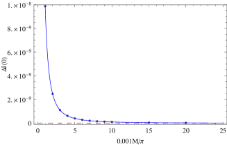
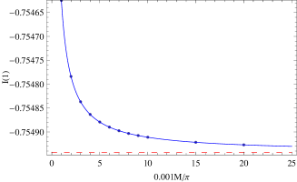
Figure 2: In the left figure, we plot the difference between our numerical results for $\ell=0$ (the data points and their best fit shown using solid line), and the theoretical value $E_{\mbox{\footnotesize Cas.}}=\frac{-\pi}{12}$ (in units $\frac{\hbar c}{2a}=1$) as a function of the cutoff $M$, as explained in the text. Note that, our numerical values asymptotically approach the theoretical value. In the right part of the figure we show our numerical results for the case $\ell=1$ (the data points and their best fit shown using solid line). For both figures the asymptotic values are obtained by fitting a sum of polynomials ($r^{n}$) with $n=\{-5,...,0\}$ and are shown using dashed lines.

The case $\ell=0$ also serves a secondary purpose, which is a crucial part for the rest of our numerical analysis. For this case the frequencies are proportional to integer multiples of $\pi$ and the original expression for the Casimir energy, Eq. (1), can be computed directly as follows:

$$E=\frac{\hbar}{2}\sum\limits_{s=1}^{\infty}\omega_{0,s}=\frac{\hbar c}{2}\sum\limits_{s=1}^{\infty}k_{0,s}=\frac{\hbar c}{2}\sum\limits_{s=1}^{\infty}\frac{s\pi}{a}=\frac{\hbar c\pi}{2a}\zeta(-1)\rightarrow\small{\frac{\hbar c\pi}{2a}\Big{(}\frac{-1}{12}\Big{)}}.$$ (13)

Note that in the last step indicated by arrow we have used the analytic continuation of the zeta function [7, 82]. In the left part of Fig. (2) we have plotted the difference between our numerical results for various values of the cutoff $M$, for the case $\ell=0$, and the theoretical value $\frac{-\pi}{12}$ (in units $\frac{\hbar c}{2a}=1$). As it is apparent from this figure, the asymptotic values of our numerical results exactly matches the theoretical one. This clearly shows the consistency between our numerical methods and the theoretical results obtained by analytical continuation of the zeta function. In the right part of Fig. (2), we plot the actual numerical values of the Casimir energy for $\ell=1$, since theoretical values do not exist in this case. In Table (2) all the results obtained for various values of $\ell$, up to $\ell=21$, are shown for various values of the cutoff. Note that the values indicated in the last column are the asymptotic values which correspond to the cases in which the cutoffs have been sent to infinity.

$\ell$	$M=1000\pi$	$M=5000\pi$	$M=10000\pi$	$M=15000\pi$	$M=20000\pi$	$M\to\infty$
0	-0.26179	-0.26179	-0.26179	-0.26179	-0.26179	$-\pi/12$
1	-0.75462	-0.75488	-0.75491	-0.75492	-0.75493	-0.75494
2	-1.25211	-1.25287	-1.25296	-1.25300	-1.25301	-1.25306
3	-1.75030	-1.75183	-1.75202	-1.75208	-1.75211	-1.75221
4	-2.24855	-2.25109	-2.25141	-2.25151	-2.25156	-2.25172
5	-2.74666	-2.75046	-2.75094	-2.75110	-2.75118	-2.75141
6	-3.24454	-3.24986	-3.25053	-3.25075	-3.25086	-3.25120
7	-3.74217	-3.74926	-3.75015	-3.75044	-3.75059	-3.75104
8	-4.23952	-4.24863	-4.24977	-4.25015	-4.25034	-4.25092
9	-4.73658	-4.74796	-4.74939	-4.74987	-4.75010	-4.75082
10	-5.23335	-5.24725	-5.24899	-5.24958	-5.24987	-5.25074
11	-5.72982	-5.74648	-5.74858	-5.74928	-5.74963	-5.75068
12	-6.22599	-6.24567	-6.24814	-6.24897	-6.24938	-6.25062
13	-6.72186	-6.74480	-6.74768	-6.74865	-6.74913	-6.75058
14	-7.21742	-7.24387	-7.24720	-7.24831	-7.24887	-7.25054
15	-7.71268	-7.74288	-7.74669	-7.74796	-7.74859	-7.75050
16	-8.20764	-8.24183	-8.24615	-8.24759	-8.24831	-8.25047
17	-8.70229	-8.74073	-8.74558	-8.74720	-8.74801	-8.75045
18	-9.19663	-9.23956	-9.24498	-9.24680	-9.24770	-9.25042
19	-9.69067	-9.73834	-9.74436	-9.74637	-9.74738	-9.75040
20	-10.18441	-10.23705	-10.24370	-10.24593	-10.24704	-10.25038
21	-10.67784	-10.73570	-10.74302	-10.74546	-10.74669	-10.75036

Table 2: The results of numerical integrations are listed for various values of $\ell$ and the cutoff $M$. All of these values are denoted by $I(\ell,M)$. For the last column, we define $f(\nu)=|I(\ell,\infty)|$, where $\nu=\ell+\frac{1}{2}$

It can be shown that the integral (2) is an odd function of $\nu$. An appropriate ansatz for the integral, which can be obtained by fitting its asymptotic values reported in Table (2), is

$$\begin{array}[]{ll}f(\nu)=A\nu+B\nu^{-1}+C\nu^{-3}+D\nu^{-5}+\mathcal{O}(\nu)^{-7},\hskip 14.22636pt\mbox{where}\hskip 14.22636pt\nu=\ell+\frac{1}{2}\end{array}$$ (15)

where $f(\nu)$ indicates the absolute value of the asymptotic values of our numerical integration ($I(\ell,M)$) recorded in the last column of Table (2), and $A$,$B$,$C$ and $D$ are the unknown coefficients to be determined from the data. To find these coefficients we fit an increasing sequence of data points to the above ansatz, and then find the overall asymptotic values of these coefficients. To be more concrete, we fit the values of the following set of sets of data points: $\ell$= $\{\{1,2,3,4,5\},\{1,2,3,4,5,6\},...,\{1,2,3,...,21\}\}$, and for each set (which contains $N$ data points) we find the corresponding coefficients $A_{N}$, $B_{N}$,$C_{N}$ and $D_{N}$.

In Fig.(3) we plot $A_{N}$, $B_{N}$,$C_{N}$ and $D_{N}$ as a function of $N$. These four graphs clearly show that there are asymptotic values for the coefficients which we denote by $A_{\infty}$, $B_{\infty}$, $C_{\infty}$ and $D_{\infty}$. We had $17$ sets of data points for each graph, we fit a polynomial with terms $N^{-j}$ with $j\in\{-5,-4,...,0\}$, and obtained the asymptotic values,

$$\begin{array}[]{ll}A_{\infty}=0.50000\hskip 14.22636pt,\hskip 14.22636ptB_{\infty}=0.00781\hskip 14.22636pt,\hskip 14.22636ptC_{\infty}=-0.00105\hskip 14.22636pt,\hskip 14.22636ptD_{\infty}=0.00034,\end{array}$$ (17)

so we have,

$$\begin{array}[]{ll}f(\nu)=A_{\infty}\nu+B_{\infty}\nu^{-1}+C_{\infty}\nu^{-3}+D_{\infty}\nu^{-5}+\mathcal{O}(\nu)^{-7}\hskip 28.45274pt\small{\ell>0}.\end{array}$$ (19)

Before proceeding with our calculation, it is interesting to mention that $f(\nu)$ has the following reported asymptotic expansion (Eq. (3.2) in Ref. [70]),

$$\small{f(\nu)=\frac{\nu}{2}+\frac{1}{128\nu}-\frac{35}{32768\nu^{3}}+\frac{565}{1048576\nu^{5}}+\mathcal{O}(\nu)^{-7}}\hskip 28.45274pt\small{\ell>0}.$$ (20)

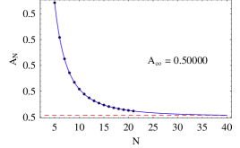
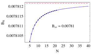
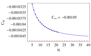
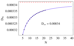
Figure 3: The plots of $A_{N}$, $B_{N}$,$C_{N}$ and $D_{N}$ as a function of $N$, as explained in the text. These four graphs clearly show that there are asymptotic values for the coefficients which we denote by $A_{\infty}$, $B_{\infty}$, $C_{\infty}$ and $D_{\infty}$.

Comparing these two expressions, it is obvious that they are equivalent, to within the numerical accuracy of our calculation. Now we can substitute our optimal functional form obtained for the integral, Eq. (19), into Eq. (2) to obtain,

$$\footnotesize{E_{\mbox{\footnotesize Cas.}}=\frac{\hbar c}{2a}\sum\limits_{s=1}^{\infty}s\pi+\frac{-\hbar c}{2a}\bigg{(}\sum\limits_{\ell=1}^{\infty}2\nu f(\nu)\bigg{)}-\{a\to R/\eta\}}$$

$$=\frac{\hbar c}{2a}\Bigg{[}\zeta(-1)\pi-2A_{\infty}\zeta(-2,3/2)-2B_{\infty}\zeta(0,3/2)-2C_{\infty}\zeta(2,3/2)$$

$$-2D_{\infty}\zeta(4,3/2))\Bigg{]}-\{a\to R/\eta\}$$

$$=\frac{\hbar c}{2a}\Bigg{[}\frac{-\pi}{12}-2A_{\infty}\bigg{(}\frac{-1}{4}\bigg{)}-2B_{\infty}\big{(}-1\big{)}-2C_{\infty}(\frac{\pi^{2}}{2}-4)$$

$$-2D_{\infty}(\frac{\pi^{4}}{6}-16)\Bigg{]}-\{a\to R/\eta\},$$ (21)

where in the last step we have used the analytic continuations of the generalized zeta functions [7, 82] along with the following shift formula for the zeta functions,

$$\begin{array}[]{ll}\zeta(n,m)=\sum\limits_{k=0}^{\infty}\left(k+m\right)^{-n}=m^{-n}+\sum\limits_{k^{\prime}=0}^{\infty}\left(k^{\prime}+m+1\right)^{-n}=m^{-n}+\zeta({n,m+1}).\end{array}$$ (23)

Obviously, in this case the last term in Eq. (3) goes to zero as $R\to\infty$. We have checked that we can obtain the same finite result, without resorting to any analytic continuation, using the Abel-Plana summation formula. We have separated the $\ell=0$ term from the rest of the summation over $\ell$, primarily because the value of the integral for $\ell=0$ dose not follow as closely as we like the pattern of other data points. We have checked that our shift formula allows us to single out this term, even when we need to analytically continue the zeta functions.

Our final result for the Casimir energy for a massless scalar field with Dirichlet boundary condition in a three dimensional sphere is,

$$\hskip 71.13188ptE_{\mbox{\footnotesize Cas.}}=+0.00562\left(\frac{\hbar c}{2a}\right).$$ (24)

This result has been obtained numerically and is the same as the previously reported result  [positive., 70, 71], which were obtained by different numerical methods, to within $0.2\%$.

4 Conclusion

In this paper, the Casimir energy for a massless scalar field in a sphere with radius $a$ with Dirichlet boundary condition is computed in three spatial dimensions. This energy has been computed using the BSS which is based on confining the original sphere inside a concentric larger sphere and computing the difference between the vacuum energies of two configurations which differ only by the size of the inner spheres. Finally, the radii of all the spheres except the original one go to infinity. Our result shows that the Casimir energy for a massless scalar field in a cube and a sphere have indeed opposite signs, contrary to the case of the EM field. As mentioned in the Introduction, and explicitly shown in Table (1), the sign of the Casimir energy for closed surfaces depends crucially on the type of field considered, the boundary conditions imposed, and the details of the geometry and not merely the topology. To be more specific, the claim that the sign of the Casimir energy should not have a significant dependency on the details of the shapes of the vessels [21, 74, 75] is, much to our surprise, not true.

Appendix A The Imposition of the Boundary Conditions

In this Appendix, we show how the imposition of Dirichlet boundary condition on the inner and outer spheres relates the root indices, $s$ and $S$, and the wave-vectors $k_{\ell,s}\left(a\right)$ and $K_{\ell,S}\left(a,R\right)$, which appear in the main regulated expression for the Casimir energy, Eq. (3). For the configuration A, we obtain the following condition for the inner sphere

$$j_{\ell}\left(ak_{\ell,s}\left(a\right)\right)=0.$$ (A.1)

That is $k_{\ell,s}(a)$ is the $s$th zero of $j_{\ell}(ak_{\ell,s}(a))$. The ranges of the values of angular momentum and inner root indices are $\ell=\{0,1,2,3,...\}$ and $s=\{1,2,3,...\}$. Similarly, the following relationship can be obtained by combining the results of the imposition of the Dirichlet boundary conditions on the two surfaces confining the annular region,

$$\displaystyle\frac{j_{\ell}\left(aK_{\ell,S}\left(a,R\right)\right)}{n_{\ell}\left(aK_{\ell,S}\left(a,R\right)\right)}-\frac{j_{\ell}\left(RK_{\ell,S}\left(a,R\right)\right)}{n_{\ell}\left(RK_{\ell,S}\left(a,R\right)\right)}=0,$$ (A.2)

where $K_{\ell,S}(a,R)$ is the $S$th zero of Eq. (A.2). The ranges of the values of angular momentum and annular root indices are $\ell=\{0,1,2,3,...\}$ and $S=\{1,2,3,...\}$. In order to find the relationship between the root indices and the wave-vectors, we use the following relationships between the spherical Bessel functions, trigonometric functions, and polynomials in $x^{-1}$,

$$\begin{array}[]{l}\vspace{0.3cm}xj_{\ell}(x)=\sin\left(x-\frac{1}{2}\ell\pi\right)A_{\ell}(x)+\cos\left(x-\frac{1}{2}\ell\pi\right)B_{\ell}(x),\\ xn_{\ell}(x)=-\cos\left(x-\frac{1}{2}\ell\pi\right)A_{\ell}(x)+\sin\left(x-\frac{1}{2}\ell\pi\right)B_{\ell}(x),\end{array}$$ (A.5)

where

$$A_{\ell}(x)=\sum\limits_{r=0}^{[\frac{1}{2}\ell\,]}\frac{\left(-1\right)^{r}(\ell+2r)!}{(2r)!(\ell-2r)!}\left(4x^{2}\right)^{-r},$$

$$B_{\ell}(x)=\frac{1}{2x}\sum\limits_{r=0}^{[\frac{1}{2}\ell-\frac{1}{2}\,]}\frac{\left(-1\right)^{r}(\ell+2r+1)!}{(2r+1)!(\ell-2r-1)!}\left(4x^{2}\right)^{-r}.$$ (A.6)

Using Eqs. (A.5,A) and Eq. (A.1), we obtain the following nonlinear relation between integer $s$ and $k_{\ell,s}\left(a\right)$,

$$ak_{\ell,s}\left(a\right)-\frac{1}{2}\ell\pi=\pi s-\arctan\left[\frac{B_{\ell}\left(ak_{\ell,s}\left(a\right)\right)}{A_{\ell}\left(ak_{\ell,s}\left(a\right)\right)}\right],$$ (A.7)

which can be simplify to,

$$\pi s=-\arctan\left[\frac{j_{\ell}\left(ak_{\ell,s}\left(a\right)\right)}{n_{\ell}\left(ak_{\ell,s}\left(a\right)\right)}\right].$$ (A.8)

Similarly, we can repeat analogous steps to obtain an equation for integer $S$ as a function of $K_{\ell,S}(a,R)$ for the annular region,

$$\pi S=\arctan\left[\frac{j_{\ell}\left(aK_{\ell,S}\left(a,R\right)\right)}{n_{\ell}\left(aK_{\ell,S}\left(a,R\right)\right)}\right]-\arctan\left[\frac{j_{\ell}\left(RK_{\ell,S}\left(a,R\right)\right)}{n_{\ell}\left(RK_{\ell,S}\left(a,R\right)\right)}\right].$$ (A.9)

Comparing Eq. (A.8) with Eq. (A.9) we obtain the following relationship between the root indices,

$$S_{\ell}\left(a,R,K\right)=s_{\ell}\left(R,K\right)-s_{\ell}\left(a,K\right).$$ (A.10)

Note that, in this equation the values of the root indices $s$, $S$, and the wave-vector $K$ can be thought of as having been analytically continued to non-integer values.

Appendix B Implementing the $R\to\infty$ Limit

In this Appendix, we show that in the limit $R\to\infty$, the contribution to the Casimir energy, reflected by the last two terms in Eq. (3), can be greatly simplified. This is due to the fact that, as we shall show, most of the infinities coming from the annular regions cancel due to BSS, and all of the remaining finite terms approach zero. Using the EMSF, the contribution of the annular region in Eq. (3) is,

$$\begin{array}[]{ll}\vspace{0mm}\displaystyle\sum\limits_{S=1}^{\infty}\left[K_{\ell,S}\left(a,R\right)\,g\left(\lambda K_{\ell,S}\left(a,R\right)\right)-K_{\ell,S}\left(R/\eta,R\right)\,g\left(\lambda K_{\ell,S}\left(R/\eta,R\right)\right)\right]\\ \vspace{2mm}=\displaystyle\int_{S=1}^{\infty}dS\left[K_{\ell}\left(a,R,S\right)\,g\left(\lambda K_{\ell}\left(a,R,S\right)\right)-K_{\ell}\left(R/\eta,R,S\right)\,g\left(\lambda K_{\ell}\left(R/\eta,R,S\right)\right)\right]\\ \vspace{2mm}+\displaystyle\frac{1}{2}\left[K_{\ell,1}\left(a,R\right)\,g\left(\lambda K_{\ell,1}\left(a,R\right)\right)-K_{\ell,1}\left(R/\eta,R\right)\,g\left(\lambda K_{\ell,1}\left(R/\eta,R\right)\right)\right]\\ \vspace{2mm}\displaystyle+\sum\limits_{r=1}^{r=N}\frac{B_{2r}}{(2r)!}\left\{\frac{d^{2r-1}}{dS^{2r-1}}\Bigg{[}K_{\ell}(a,R,S)g(\lambda K_{\ell}(a,R,S))-K_{\ell}(R/\eta,R,S)g(\lambda K_{\ell}(R/\eta,R,S))\Bigg{]}\right\}_{S=1}\\ \vspace{2mm}\displaystyle-\int_{S=1}^{\infty}dS\,B_{2N}\left(S-[S]\right)\\ \displaystyle\times\frac{d^{2N}}{dS^{2N}}\Bigg{[}K_{\ell}\left(a,R,S\right)\,g\left(\lambda K_{\ell}\left(a,R,S\right)\right)-K_{\ell}\left(R/\eta,R,S\right)\,g\left(\lambda K_{\ell}\left(R/\eta,R,S\right)\right)\Bigg{]}.\end{array}$$ (B.7)

Here we show that the last three terms in the right hand side (rhs) of Eq. (B.7) give no contribution to the Casimir energy. In fact, in the limit $R\to\infty$, all terms in the rhs of Eq. (B.7), except for the first integral, cancel each other due to BSS or vanish entirely. In order to show the vanishing of these terms, we have to prove two things. First, each of these terms decreases rapidly as a function of $\ell$, so that when it is summed over $\ell$ with a pre-factor of $2\ell+1$ it will not give a divergent contribution. Second, each term approaches zero in the limit $R\to\infty$.

We start with the second term. For the small values of $\ell$, the first root goes to zero as $R^{-1}$. For large values of $\ell$, the first root $K_{\ell,1}(R/\eta,R)$ behaves like,

$$K_{\ell,1}(R/\eta,R)=k_{\ell,1}(R)+\frac{\epsilon}{R}$$ (B.8)

where

$$\epsilon\sim\frac{\nu^{1/3}}{1.23\eta}e^{-2\nu(\beta_{\nu}-\tanh\beta_{\nu})}\hskip 28.45274pt\textmd{, and}\hskip 28.45274pt(\cosh\beta_{\nu})^{-1}\sim\eta^{-1}[1+\mathcal{O}(\nu^{-2/3})].$$ (B.9)

and $\nu=\ell+1/2$. Therefore, the second term becomes,

$$\frac{1}{2}\Bigg{[}\left(k_{\ell,1}(R)+\frac{\epsilon}{R}\right)e^{-\lambda\left(k_{\ell,1}(R)+\frac{\epsilon}{R}\right)}-\left(k_{\ell,1}(R)+\frac{\epsilon^{\prime}}{R}\right)e^{-\lambda\left(k_{\ell,1}(R)+\frac{\epsilon^{\prime}}{R}\right)}\Bigg{]}$$

$$=\frac{1}{2}\Bigg{[}\left(k_{\ell,1}(R)+\frac{\epsilon}{R}\right)-\lambda\left(k_{\ell,1}(R)+\frac{\epsilon}{R}\right)^{2}+...$$ (B.10)

$$\hskip 5.69046pt-\left(k_{\ell,1}(R)+\frac{\epsilon^{\prime}}{R}\right)+\lambda\left(k_{\ell,1}(R)+\frac{\epsilon^{\prime}}{R}\right)^{2}+...\Bigg{]}\sim\mathcal{O}(\epsilon/R)-\mathcal{O}(\epsilon^{\prime}/R),$$

For obtaining the second line we have expanded the exponentials since $\lambda$ eventually approaches zero. As shown in Eq. (B.9) the numerators $\epsilon$ and $\epsilon^{\prime}$ decrease exponentially in $\ell$, and the entire term goes to zero in the limit $R\to\infty$.

An analogous argument can be used for the third term in the rhs of Eq. (B.7). In the neighborhood of $S=1$, we have the following relationship between the wave-vectors,

$$K_{\ell}(a,R,S)=k_{\ell}(R,S)+\delta_{\ell}(a,R,S).$$ (B.11)

where $\delta_{\ell}(a,R,S)$ decreases exponentially with increasing $\ell$ and vanishes as $R\to\infty$. Analogous relationship holds for any derivatives of the wave-vectors. In fact, all terms which depend only upon the outer radius $R$ (and not on the inner ones $a$ or $R/\eta$) are canceled due to BSS, and the remaining terms go to zero as $R\to\infty$.

Now, we proceed to the fourth term. Here, we show that the remaining integral decreases rapidly with increasing $\ell$. We rewrite the integral as

$$\Bigg{|}\int_{S=1}^{\infty}dS\,B_{2N}\left(S-[S]\right)\frac{d^{2N}}{dS^{2N}}\Bigg{[}K_{\ell}\left(a,R,S\right)\,g\left(\lambda K_{\ell}\left(a,R,S\right)\right)-\{a\to R/\eta\}\Bigg{]}\Bigg{|}$$

$$\leq\frac{|B_{2N}|}{(2N)!}\int_{S=1}^{S=S^{*}}dS\left|\frac{d^{2N}}{dS^{2N}}\Bigg{[}K_{\ell}\left(a,R,S\right)\,g\left(\lambda K_{\ell}\left(a,R,S\right)\right)-\{a\to R/\eta\}\Bigg{]}\right|$$

$$+\frac{|B_{2N}|}{(2N)!}\int_{S=S^{*}}^{S=\infty}dS\left|\frac{d^{2N}}{dS^{2N}}\left[K_{\ell}\left(a,R,S\right)\,g\left(\lambda K_{\ell}\left(a,R,S\right)\right)\right]\right|$$

$$+\frac{|B_{2N}|}{(2N)!}\int_{S=S^{*}}^{S=\infty}dS\left|\frac{d^{2N}}{dS^{2N}}\left[K_{\ell}\left(R/\eta,R,S\right)\,g\left(\lambda K_{\ell}\left(R/\eta,R,S\right)\right)\right]\right|$$ (B.12)

where $S^{*}=S_{\ell}(R/\eta,R,\nu/b)$ and $b$ is constrained by: $R/\eta<b<R$. For large values of $\ell$, we can repeat analogous arguments given above to show that for the first integral the terms of the integrand which depend only upon the outer radius $R$, are canceled due to BSS, and the result of the integration of the remaining terms decrease exponentially with increasing $\ell$ and vanish for $R\to\infty$. As for the second term in the rhs of Eq. (B), the high order derivatives of the wave-vector $K_{\ell}\left(a,R,S\right)$ for large value of $\ell$ are,

$$\frac{d^{m}K_{\ell}\left(a,R,S\right)}{dS^{m}} = \mathcal{O}({\nu}^{1-m}),\hskip 14.22636pt\mbox{for}\hskip 14.22636pt\nu/R\ll K_{\ell}\left(a,R,S\right)\ll\nu/a$$ (B.13)

$$= \mathcal{O}(\nu^{-m/3}),\hskip 9.95863pt\mbox{for}\hskip 14.22636ptK_{\ell}\left(a,R,S\right)\sim(\nu+\tau\nu^{1/3})/a$$

$$= \mathcal{O}(\nu^{1-m}),\hskip 14.22636pt\mbox{for}\hskip 14.22636pt\nu/a\ll K_{\ell}\left(a,R,S\right)$$

where $\nu=\ell+1/2$ and $m>1$. Thus if a sufficient number of terms are taken in the EMSF (Eq. (B.7)) the high order derivatives of the wave-vector, $K_{\ell}$, decrease with increasing $\nu$. Moreover, when derivatives operate on the damping factors, $g(\lambda K_{\ell}\left(a,R,S\right))=e^{-\lambda K_{\ell}\left(a,R,S\right)}$, each derivative extracts a factor of $\lambda$,

$$\frac{d}{dS}g(\lambda K_{\ell}\left(a,R,S\right))\sim\lambda\mathcal{O}\Big{[}\frac{1}{R}g(\lambda K_{\ell}\left(a,R,S\right))\Big{]}.$$ (B.14)

Now, if $N$ in Eq. (B.7) is chosen to be large enough, each term arising from $\left|\frac{d^{2N}}{dS^{2N}}\left[K_{\ell}\left(a,R,S\right)\,g\left(\lambda K_{\ell}\left(a,R,S\right)\right)\right]\right|$, decreases rapidly with increasing $\nu$ or has many factors of $\lambda$. The terms which have factors of $\lambda$ approach zero when $\lambda$ goes to the zero, and for any remaining terms, their integral decrease rapidly as a function of $\nu$ and the contribution of these terms approach zero in the limit $R\to\infty$. Analogous argument can be repeated for the last integral in the rhs of Eq. (B), only with the replacement $a\to R/\eta$. Therefore, we have shown that the left hand side of Eq. (B) approaches zero. Finally, the result of this analysis is that the only contribution coming from the annular region is the integral term in the rhs of Eq. (B.7). Therefore, the summation in the Eq. (3) can be replaced by its integral.

References

References

- [1] H. B. G. Casimir and D. Polder, Phys. Rev. 73, 360 (1948).
- [2] H. B. G. Casimir, Proc. Kon. Aa. Wet. 51, 793 (1948).
- [3] M. Bordag, U. Mohideen and V. M. Mostepanenko, Phys. Rep. 353, 1 (2001); [arXiv:quant-ph/0106045].
- [4] K. A. Milton, [arXiv:hep-th/9901011] (1999).
- [5] G. Plunien, B. Mueller, and W. Greiner, Phys. Rep. 134, 87 (1986).
- [6] K. A. Milton, The Casimir Effect: Physical Manifestations of Zero-Point Energy, (World Scientific Publishing Co. 2001).
- [7] E. Elizalde, Ten Physical Applications of Spectral Zeta Functions, Lecture Notes in Physics (Springer-Verlag, Berlin, Heidelberg 1995).
- [8] M. J. Sparnaay, Physica 24, 751 (1958).
- [9] G. Bressi, G. Carugno, R. Onfrio, G. Ruoso, Phys. Rev. Lett. 88, 041804 (2002).
- [10] S. K. Lamoreaux, Phys. Rev. Lett. 78, 5 (1997).
- [11] R. S. Decca, D. López, H.B. Chan, E. Fischbach, D.E. Krause, and C.R. Jamell, Phys. Rev. Lett. 94, 240401 (2005).
- [12] R. S. Decca, D. López, E. Fischbach, G.L. Klimchitskaya, D.E. Krause, and V.M. Mostepanenko, Ann. Phys., 318, 37 (2005).
- [13] B. Geyer, G. L. Klimchitskaya, and V. M. Mostepanenko, Int. J. Mod. Phys. A 16, 3291 (2001).
- [14] D. A. R. Dalvit, F.C. Lombardo, F.D. Mazzitelli, and R. Onofrio, Europhys. Lett. 67, 517 (2004).
- [15] K. Kirsten, Spectral Functions in Mathematics and Physics, (Chapman Hall/CRC, London, 2002).
- [16] S. Hacyan, R. Jauregui, and C. Villarreal, Phys. Rev. A 47, 4204 (1993).
- [17] H. Cheng, J. Phys. A: Math. Gen. 35, 2205 (2002).
- [18] G. J. Maclay, Phys. Rev. A 61, 052110 (2000).
- [19] A. Gusso, and A. G. M. Schmidt, Brazilian Journal of physics 36, 1B 168 (2006).
- [20] J. R. Ruggiero, A. Villani and A. H. Zimerman, J. Phys. A: Math. Gen. 13, 761 (1980).
- [21] W. Lukosz, Physica, 56, 109 (1971).
- [22] P. A. M. Neto, J. Opt. B: Quantum Semiclass. 7, s86 (2005).
- [23] F. D. Mazzitelli, M. J. Sanchez, N. N. Scoccola, and J. von Stecher, Phys. Rev. A 67, 013807 (2003).
- [24] D. A. R. Dalvit, F. C. Lombardo, F. D. Mazzitelli, and R. Onofrio, Phys. Rev. A 74, 020101 (2006).
- [25] V. V. Nesterenko, and I. G. Pirozhenko, Phys. Rev. D 60, 125007 (1999).
- [26] Kimball A. Milton, A. V. Nesterenko, and V. V. Nesterenko, Phys. Rev. D 59, 105009 (1999).
- [27] Francisco D. Mazzitelli, María J. Sánchez, Norberto N. Scoccola, and Javier von Stecher, Phys. Rev. A 67, 013807 (2003).
- [28] Peter Gosdzinsky, and August Romeo, Phys. Lett. B 441, 265 (1998).
- [29] R. B. Rodrigues, N. F. Svaiter, Physica A 328, 466 (2003).
- [30] M. Bordag, E. Elizalde, K. Kirsten, and S. Leseduarte, Phys. Rev. D 56, 4896 (1997).
- [31] E. Elizalde, M. Bordag, and K. Kirsten, J. Phys. A: Math. Gen. 31, 1743 (1998).
- [32] C. M. Bender, and K. A. Milton, Phys. Rev. D 50, 6547 (1994).
- [33] K. Poppenhaeger, S. Hossenfelder, S. Hofmann, M. Bleicher, Phys. Lett. B 582, 1 (2004).
- [34] Carlos A. R. Herdeiro, Raquel H. Ribeiro, and Marco Sampaio, Int. J. Mod. Phys. A 24, 1821 (2009).
- [35] A. A. Saharian, and M. R. Setare, Int. J. Mod. Phys. A 19, 4301 (2004).
- [36] A. A. Saharian, and E. R. Bezerra de Mello, Int. J. Mod. Phys. A 20, 2380 (2005).
- [37] F. Caruso, N. P. Neto, B. F. Svaiter, and N. F. Svaiter, Phys. Rev. D 43, 1300 (1991).
- [38] R. M. Cavalcanti, Phys. Rev. D 69, 065015 (2004).
- [39] A. Edery, and I. MacDonald, JHEP 09, 005 (2007).
- [40] H. Alnes, F. Ravndal, I. K. Wehus, and K. Olaussen, Phys. Rev. D 74, 105017 (2006).
- [41] M. P. Hertzberg, R. L. Jaffe, M. Kardar, and A. Scardicchio, Phys. Rev. Lett. 95, 250402 (2005).
- [42] X. Li, H. Cheng, J. Li, and X. Zhai, Phys. Rev. D 56, 2155 (1997).
- [43] A. Chodos, R.L. Jaffe, K. Johnson, C.B. Thorn, and V. Weisskopf, Phys. Rev. D 9, 3471 (1974).
- [44] R. K. Bhaduri, Models of the Nucleon (Addison-Wesley, Redwood City, California, 1988).
- [45] Kimball A. Milton, Phys. Rev. D 22, 1444 (1980).
- [46] Kimball A. Milton, Phys. Rev. D 22, 1441 (1980).
- [47] G. Lambiase, V. V. Nesterenko, and M. Bordag, [arXive:hep-th:/9812059v1] (1998).
- [48] A. Romeo, Phys. Rev. D 52, 7308 (1995).
- [49] M. Bordag, E. Elizalde, and K. Kirsten, J. Math. Phys. 37, 895 (1996).
- [50] R. Garattini, TSPU Vestnik 44N7:72 (2004), [arXiv:gr-qc/0409016v1].
- [51] E. Elizalde, Phys. Lett. B 516, 143 (2001).
- [52] E. Elizalde, J. Phys. A 39, 6299 (2006).
- [53] F. Bauer, M. Lindner, and G. Seidl, JHEP 05, 026 (2004).
- [54] Cheng Hong-Bo, Chin. Phys. Lett.22, 2190 (2005).
- [55] G. Mahajan, S. Sarkar, and T. Padmanabhan, Phys.Lett. B 641, 6 (2006).
- [56] E. Elizalde, J. Math. Phys. 35, 3308 (1994).
- [57] F. De Martini, M. Marrocco, and P. Mataloni, Phys. Rev. A 43, 2480 (1991).
- [58] M. Krech, and S. Dietrich, Phys. Rev. Lett. 66, 345 (1991).
- [59] M. Krech, and S. Dietrich, Phys. Rev. Lett. 67, 1055 (1991).
- [60] F. De Martini and G. Jacobovitz, Phys. Rev. Lett. 60, 1711 (1988).
- [61] D.C. Roberts and Y. Pomeau, Phys. Rev. Lett. 95, 145303 (2005).
- [62] C. Barceló, S. Liberati and M. Visser, Class. Quantum Grav. 18, 3595 (2001).
- [63] A. Edery, Phys. Rev. D 75, 105012 (2007).
- [64] T. H. Boyer, Phys. Rev. 174, 1764 (1968).
- [65] K. A. Milton, L. L. De Raad Jr., and J. Schwinger, Ann. Phys. (N.Y.) 115, 388 (1978).
- [66] Peter Gosdzinsky, and August Romeo, Phys. Lett. B 441, 265 (1998).
- [67] I. Brevik, V.V. Nesterenko, and I.G. Pirozhenko, J. Phys. A: Math. Gen. 31, 8661 (1998).
- [68] S. Leseduarte, and August Romeo, Ann. Phys. 250, 448 (1996).
- [69] G. Cognola, E. Elizalde, and Klaus Kirsten, J. Phys. A: Math. Gen. 34, 7311 (2001).
- [70] V. V. Nesterenko, and I. G. Pirozhenko, Phys. Rev. D 57, 2 (1998).
- [71] M. E. Bowers and C. R. Hagen, Phys. Rev. D 59, 025007 (1998).
- [72] X. Li and X. Zhai, J. Phys. A: Math. Gen. 34, 11053 (2001).
- [73] Luiz A. Manzoni, Walter F. Wreszinski, Phys. Lett. A 292, 156 (2001).
- [74] J. Ambjørn and S. Wolfram, Ann. Phys. (N.Y.) 147, 1 (1983).
- [75] C. Peterson, T. H. Hansson, and K. Johnson, Phys. Rev. D 26, 415 (1982).
- [76] M. Reuter and W. Dittrich, Eur. J. Phys. 6, 33 (1985).
- [77] R. Cavalcanti, Phys. Rev. D 69, 065015 (2004).
- [78] M. P. Hertzberg, R. L. Jaffe, M. Kardar, and A. Scardicchio, Phys. Rev. D 76, 045016 (2007).
- [79] M. A. Valuyan, R. Moazzemi, and S. S. Gousheh, J. Phys. B: At. Mol. Opt. Phys. 41, 145502 (2008); [arXiv:hep-th/0806.1628v1].
- [80] R. Moazzemi, S. S. Gousheh, JHEP 09, 029 (2008); [arXiv:hep-th/0708.4127v1].
- [81] R. Moazzemi, S. S. Gousheh, Phys. Lett. B 658, 255 (2008); [arXiv:hep-th/0708.3428v2].
- [82] E. Elizalde, S. D. Odintsov, A. Romeo, A. A. Bytsenko and S. Zerbini, Zeta Regularization techniques with Applications, (World Scientific Publishing Co. Pte. Ltd., Singapore, 1994).