Ground State Geometry of Binary Condensates in Axisymmetric Traps
Abstract
We show that the ground state interface geometry of binary condensates in the phase separated regime undergoes a smooth transition from planar to ellipsoidal to cylindrical geometry. This occurs for condensates with repulsive interactions as the trapping potential is changed from prolate to oblate. The correct ground state geometry emerges when the interface energy is included in the energy minimization. Where as energy minimization based on Thomas-Fermi approximation gives incorrect geometry.
pacs:
03.75.Mn, 03.75.Hh, 67.85.BcI Introduction
Two species Bose-Einstein condensate (TBEC), consisting of two different hyperfine spin sates of 87Rb, was first observed by Myatt et al Myatt . Since then, TBECs of different atomic species (41K and 87Rb) Modugno and of different isotopes of the same atomic species Papp have been experimentally realized. This has led to several experimental and theoretical investigations on different aspects of TBECs. The remarkable feature of TBECs which is absent in a single component Bose-Einstein condensates (BECs) is the phenomenon of phase separation. In Thomas-Fermi approximation (TFA), the phase separation occurs when all the inter atomic interactions are repulsive and the inter species repulsion exceeds the geometric mean of the intra species repulsive interactions.
Depending upon the properties of the condensates and trapping potential parameters, the ground state of TBECs assumes a configuration which minimizes the total energy. The structure of the ground state plays an important role in dynamical phenomena like Rayleigh–Taylor Gautam ; Sasaki instability, Kelvin-Helmholtz instability Takeuchi , pattern formation at the interface Saito etc. It was recently demonstrated that quantum Rayleigh–Taylor instability can be observed in a very controlled way with TBECs in cigar shaped traps Gautam .
In the phase separated regime, the interface energy of the two component species defines the geometry of the ground state. In a previous work, the ground state geometry of TBECs was examined within the TFA Ho that is without the interface energy. In later works, Timmermans ; Ao ; Barankov the contribution from the interface energy was incorporated. From these it is observed that the analytic approximations for interface energy are not sufficient enough to explain the experimental results of strongly segregated ground states Papp . A recent work Schaeybroeck reported a more accurate determination of the interface energy. It explains the stationary state geometry of the strongly segregated TBECs more precisely.
In this paper we provide a semi-analytic scheme to determine the stationary state structure of TBEC in axisymmteric traps. For this, we follow the ansatz adopted in Ref. Trippenbach i.e. to minimize the total energy of TBEC with fixed number of particles of each species in TFA. In section II of the manuscript, we identify three geometries which a TBEC can assume depending on the trapping potential parameters. Based on TFA, we provide a semi-analytic scheme to determine the stationary state parameters of the ground state for each of these three geometries. In section III, we analyze the crucial role played by the interface energy in determining the ground state structure of the TBEC.
II TBEC in Axisymmetric Traps
We consider TBEC in axisymmetric trapping potentials
| (1) |
where is the species index, and and are the anisotropy parameters. In the mean field approximation, the stationary state solution of binary condensate is described by a set of coupled Gross-Pitaevskii equations
| (2) |
here and are species indices; with as mass and as s-wave scattering length, is the intra-species interaction; with as reduced mass and as inter-species scattering length, is the inter-species interaction term and is the chemical potential of the th species.
When the number of atoms are large, the TFA is applicable to obtain the stationary state solutions of Eq.(2). In this limit the kinetic energy is neglected in comparison to interaction energy. We consider the interaction parameter , such that the two components are phase separated. That is, the two components occupy different regions of the trapping potentials. Neglecting the overlap between the species, stationary state solutions within TFA are
| (3) |
where is fixed by the number of atoms of the corresponding species.
The total energy of the TBEC in the phase separated regime is
| (4) | |||||
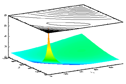
Depending upon the anisotropy parameters, the TBEC can have three distinct spatial distributions in axisymmetric traps. The distinguishing feature of these structures is the geometry of the interface, which can be planar, cylindrical or ellipsoidal. The smooth transition of interface geometry, for the TBEC of 85Rb-87Rb mixture, from planar to ellipsoidal and finally to cylindrical is shown in Fig. 1. These features are most prominent when the TBEC is strongly segregated and for the detailed examination of our scheme we choose 85Rb-87Rb experiments of Papp et al Papp . Where two of the geometries, planar and ellipsoidal, were observed.
II.1 Planar interface
It has been observed experimentally Papp that in cigar shaped traps () the TBEC assumes a sandwich structure with planar interface between the two species. In this structure the phase separation occurs along the axial direction, with the weakly interacting component sandwiched by the strongly interacting one. There are two realizations of this: coincident and shifted trapping potentials.

II.1.1 Coincident trap centers
An idealized choice of is with coincident centers. If are the locations of the planes separating the two components and , the axial size of binary condensate. Then the problem of determining the structure of the TBEC is equivalent to calculating . If and are the number of atoms and radial size of the th species respectively, then
| (5) |
From Eq.(3), we get
Similarly, the total energy in Eq.(4) is
| (7) | |||||
Here, is determined by variational minimization of with as the variational parameter and constraints that , and satisfy Eq.(II.1.1) for fixed . In the constraint equations, we invert the expression of and obtain as a function of . However, inverting to calculate is nontrivial. Hence, we implement the minimization numerically.
As mentioned earlier we consider the TBEC of 85Rb-87Rb with . The scattering lengths , and are from the experimental results of Wieman and collaborators Papp . Like wise the anisotropy parameters and trap frequency are , , and Hz respectively. From here on this choice of parameters is referred as the set a. For these parameters, the minima of occurs at . This is in very good agreement with the value of obtained from the numerical solution Muruganandam of Eq.(2). The contour plots showing the absolute value of wave functions of 85Rb and 87Rb, obtained by numerically solving Eq.(2), are shown in first image from left in upper panel of Fig. 1.
II.1.2 Separated trap centers
In the experimental realizations, the gravitational potential and tilts in the external field configurations tends to separate the minima of the effective potentials. Normally, in cigar shaped traps, the tilt angle is small and separation is effectively along the axial direction. Then potentials with separation are
| (8) |
Due to the lack of axial symmetry, and are the two planes separating the two components. These, and , are the parameters to minimize . Like in the previous subsection , and can be evaluated and are presented in the appendix. For the parameter set a and m, the minima of occurs when and are and respectively. The overall trend of is shown in Fig. 2.
II.2 Ellipsoidal Interface
As the anisotropy parameter is increased, beyond a critical value the interface geometry change from planer to ellipsoidal. Where one species envelopes the other. This is the preferred interface geometry, for the phase separated TBEC in axisymmteric traps, without interface energy. Consider trapping potentials with coincident centers, if and are equatorial (along radial direction) and polar (along axial direction) radii of the th species respectively, then
| (9) |
From Eq.(3) and Eq.(4), we get
| (10) | |||||
| (11) | |||||
| (12) | |||||
In TFA, the profile of density has the same ellipticity as that of the trapping potential, which is a function . Then, is , further more in TFA constrains the value of . These reduce the variation parameter to only . The energy is then minimized numerically to find the equilibrium geometry of the phase separated TBEC. To examine the scheme consider the 85Rb-87Rb mixture with parameter set a and coincident trapping potentials, however take as 1.5. Then the equilibrium geometry is ellipsoidal with an equitorial radius ( ) of . This is in very good agreement with value obtained from the numerical solution of GP equations. The contour plots showing the absolute value of wave functions of 85Rb and 87Rb, obtained by numerically solving Eq.(2), are shown in second image from left in lower panel of Fig. 1.
II.3 Cylindrical interface
On further increase of , beyond another critical value , the equilibrium interface geometry is like a cylinder. Where the axis of the interface coincides with the polar axis of the trapping potentials. This occurs when i.e. in the oblate condensates. Here, the phase separation is along radial direction and analogous to planar interface in cigar shaped condensates. If is the radius of the interface cylinder, then in TFA
| (13) | |||||
Above set of equations define the stationary state of TBEC in the oblate shaped condensates. Like in the planar geometry, is the parameter of variation. To verify the scheme, we consider pan cake shaped ( ) TBEC of 85Rb-87Rb mixture in coincident traps with as 50.0 and parameter set a. Then from our scheme the equilibrium state has cylindrical interface of radius . The value from numerical solution of GP equation is . The two results are in very good agreement and validate our minimization scheme. The contour plots showing the absolute value of wave functions of 85Rb and 87Rb, obtained by numerically solving Eq.(2), are shown in third image from left in lower panel of Fig.1.
III Role of the interface energy
In the TFA calculations discussed so far, as mentioned earlier, the interface energy is neglected. Accordingly, the variational schemes we have adopted incorporate appropriate interface geometries. However, a general minimization by considering all the possible interface geometries favors the ellipsoidal interface as the equilibrium configuration. For example, though the cylindrical interface for reproduces the numerical results for TBEC of 85Rb-87Rb with parameter set a, the minimization with ellipsoidal interface has lower . This is evident from the values of , calculated over a wide range of for the three interface geometries, shown in Fig. 3.

As discussed in ref.Schaeybroeck , the planer interface observed in experiments Papp emerges as the equilibrium geometry when the interface energy is considered. When is much larger than the interface thickness, the total excess energy arising from the finite interface tension Schaeybroeck is
| (14) |
Here are the coherence lengths and , , are defined as
Here the integration is over the interface surface area. The above expression is valid provided and . In the present work we consider TBECs in strongly segregated regime with and hence the interface energy in Eq.(14) is applicable. Then the interpenetration depth is proportional to and in the limit . In this limit there is no overlap and TFA solution is an excellent approximation. The equilibrium geometry is then the one which minimizes the total energy: sum of TFA energy and .
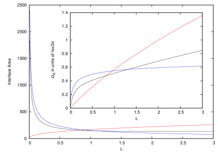
A precise determination of is essential to obtain correct geometry of the phase separated TBEC. To a very good approximation, the interface energy is proportional to interface area. The interface area in planar and cylindrical geometries are and respectively. For prolate and oblate geometries the interface areas are and and respectively. Here the ellipticity are and for prolate and oblate respectively. The interface areas in the three geometries for TBEC of 85Rb-87Rb with parameter set a, using our semi analytic scheme developed in previous section, are shown in Fig. 4. The comparative study reveals that for , planar and ellipsoidal geometries have lower interface area than the cylindrical one. Whereas for , the cylindrical and ellipsoidal geometries have lower interface areas. In these two domains the interface area of one geometry is much lower than the other two and hence interface area can decide the preferred ground state geometry. For close to one, the difference in the interface areas of the three geometries is small and surface tension is more crucial than interface area to determine the ground state geometry.
In the following subsections we examine the impact of in two domains: prolate shaped potentials ( ) and oblate shaped potentials (). For higher symmetry and simplified analysis we choose .
III.1 Prolate trapping potentials
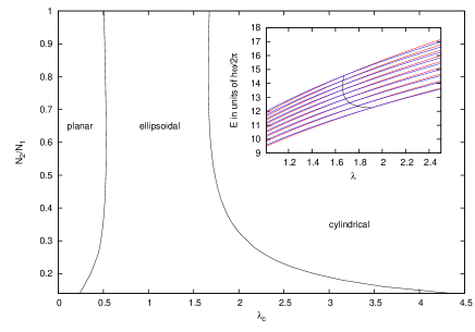
In the domain, at low values of , the ellipsoidal geometry has higher ground state energy than the planar geometry. As is increased, keeping the other parameters fixed, the ground state energies of both the geometries increase. However, the planar geometry has higher rate of increase. Then at , which is close to one, the energies of the two geometries are equal. Beyond this critical value, the energy of ellipsoidal geometry is lower and is the ground state geometry.
For the 85Rb-87Rb mixture with the parameter set a, the total energy and interface energy as functions of for the two geometries are respectively shown in Fig. 3 and Fig. 4 (inset plot). Since the value of depends on the parameters of the system, we examine the variation in as function of the ratio . For this we fix and vary . Then calculate as a function . When is decreased increases initially and then decreases. This is shown in Fig. 5.
III.2 Oblate trapping potentials
In the regime, the ellipsoidal or cylindrical interface geometry is the preferred ground state geometry. The planar interface has higher and not favored. For close to , the ellipsoidal geometry has lower energy, but looses stability as is increased. This is due to the higher rate of increase in the for ellipsoidal geometry. At the critical value and beyond, cylindrical geometry has lower total energy and takes over as the ground state geometry.
For the 85Rb-87Rb mixture with the parameter set a, the total energy and interface energy as functions of for the two geometries are shown respectively in Fig. 3 and Fig. 4 (inset plot). For the same parameter set a; the value of , first decreases and then increases on decreasing . This is shown in Fig. 5.
IV Conclusions
There are three distinct interface geometries of the ground state of TBEC in phase separated regime. We have developed a semi-analytic scheme to determine the stationary state parameters for each of these and demonstrate the validity by comparing with the numerical results. We find in TFA, when the interface energy is neglected, the ellipsoidal geometry has the lowest energy for all values of . Hence is the preferred ground state structure. In this structure one species envelopes the other and interface geometry and overall shape of the TBEC is ellipsoidal. To explain the experimentally realized stationary state structures of TBECs we include the interface surface tension. We find that minimizing total energy, sum of TFA energy and , gives the right interface geometry. Then, in our semi-analytic scheme the ellipsoidal geometry no longer has the lowest energy for all values of . For cigar shaped traps ( ), the structure with the planar interface is the ground state geometry. While for pan cake shaped traps ( ) the cylindrical interface is the ground state geometry. For the values of close to unity ellipsoidal structure is the ground state geometry.
V Appendix
In case of planar interface between the two species trapped in potentials with separated minima, the expressions for , and are:
| (15) | |||||
| (16) | |||||
| (17) | |||||
These equations reduce to those for coincident centers on substituting and .
References
- (1) C. J. Myatt, E. A. Burt, R. W. Ghrist, E. A. Cornell, and C. E. Wieman, Phys. Rev. Lett. 78, 586 (1997).
- (2) G. Modugno, M. Modugno, F. Riboli, G. Roati, and M. Inguscio, Phys. Rev. Lett. 89, 190404 (2002).
- (3) S. B. Papp, J. M. Pino and C. E. Wieman, Phys. Rev. Lett. 101, 040402 (2008).
- (4) S. Gautam, and D. Angom, arXiv:0908.4336v3.
- (5) K. Sasaki, N. Suzuki, D. Akamatsu, and H. Saito, arXiv:0910.1440v1.
- (6) H. Takeuchi, N. Suzuki, K. Kasamatsu, H. Saito, and M. Tsubota, arXiv:0909.2144v1.
- (7) H. Saito, Y. Kawaguchi, M. Ueda, Phys. Rev. Lett. 102, 230403 (2009).
- (8) Tin-Lun Ho, and V. B. Shenoy, Phys. Rev. Lett. 77, 3276 (1996).
- (9) E. Timmermans, Phys. Rev. Lett. 81, 5718 (1998).
- (10) P. Ao, and S. T. Chui, Phys. Rev. A 58, 4836 (1998).
- (11) R. A. Barankov, Phys. Rev. A 66, 013612 (2002).
- (12) B. Van Schaeybroeck, Phys. Rev. A 78, 023624 (2008).
- (13) M. Trippenbach, K. Goral, K. Rzazewski, B. Malomed, and Y. B. Band J. Phys. B 33, 4017 (2000).
- (14) P. Muruganandam, and S. K. Adhikari, Comp. Phys. Comm. 180, 1888 (2009).