Analytic structure of $\rho$ meson propagator at finite temperature

Abstract

We analyse the structure of one-loop self-energy graphs for the $\rho$ meson in real time formulation of finite temperature field theory. We find the discontinuities of these graphs across the unitary and the Landau cuts. These contributions are identified with different sources of medium modification discussed in the literature. We also calculate numerically the imaginary and the real parts of the self-energies and construct the spectral function of the $\rho$ meson, which are compared with an earlier determination. A significant contribution arises from the unitary cut of the $\pi\omega$ loop, that was ignored so far in the literature.

1 Introduction

The in-medium propagation of vector mesons, particularly the $\rho$, has been extensively studied in the literature, as reviewed in Refs.[1, 2]. The reason is, of course, that it controls the rates of dileptons and photons emitted from the hot and dense matter, created during heavy ion collisions. The recent precision measurement [3] of the in-medium $\rho$ spectral function encourages further theoretical investigation.

The effect of medium on the vacuum propagation of the vector meson is generally believed to arise from two sources [1]. One is the change in its pion cloud, given essentially by the $\pi\pi$ self-energy loop [4]. The other is the collisions suffered by the vector meson with particles in the medium. The latter effect can be calculated, broadly speaking, in two different ways. Kinetic theory expresses this collision rate in terms of the spin average of the squared scattering amplitudes [5]. This rate is simply related to the imaginary part of the self-energy of the meson [6]. The effect of collisions can also be obtained from the self-energy tensor given by the virial formula, which relates it directly to the scattering amplitude itself [7, 8, 9, 10, 11]. In the absence of scattering data, these amplitudes are generally calculated from the relevant Feynman graphs.

As shown by Weldon and others [6, 12], the two sources modifying the free propagator find a unified description in terms of contributions from branch cuts of the self-energy loop. In addition to the unitary cut, present already in the vacuum amplitude, the thermal amplitude generates a new, so-called Landau cut. While the in-medium modification by the cloud of virtual particles (mostly pions) is obtained from the unitary cut, the effect of collisions with surrounding particles is given by the Landau cut. Thus the two sources of medium modification are automatically included in the calculation, if we retain the contribution of both the cuts. The relative importance of these cuts from different graphs depend on their thresholds, besides the couplings at the vertices of the graphs.

In this work we take the one-loop self-energy graphs for the $\rho$ meson and find all the discontinuities associated with the branch cuts. The loops are formed with one internal pion line and another which may be the pion itself or any of the heavy particles, namely $\omega$, $a_{1}$ and $h_{1}$, up to a mass of about $1.25$ GeV. The resonances are treated in the narrow width approximation. The vertices of the graphs are obtained from chiral perturbation theory. The calculations are carried out in the real time version of thermal field theory.

In Sect. 2 we start with the two-point function at finite temperature of the vector current having the quantum numbers of $\rho$. Here we also review briefly the methods of chiral perturbation theory to obtain the different interaction Lagrangians needed to evaluate the self-energy loops. In Sect. 3 we describe the kinematic decomposition of the tensor amplitudes. In Sect. 4 we write explicitly the self-energies from different loops and separate these analytically into their real and imaginary parts. The cut structure of the self-energy function and the discontinuities across the cuts are obtained in Sect. 5. In Sect. 6 we evaluate numerically the imaginary and the real parts of the self-energy and construct the spectral function of the $\rho$ meson. Finally Sect. 7 discusses the assumptions and the approximations entering these evaluations. Here we also compare our results with an earlier determination. The Appendix gives a summary of the real time theory, needed in the present work.

2 Preliminaries

To study the $\rho$ meson propagator, we do not start directly with the two-point function of the $\rho$ meson field, but consider instead that of the vector current, having the quantum numbers of the $\rho$ meson. In the two-flavour $QCD$ theory, this current is given by

$$V_{\mu}^{i}(x)=\bar{q}(x)\gamma_{\mu}\frac{\tau^{i}}{2}q(x),~{}~{}~{}~{}~{}~{}q=\left(\begin{array}[]{c}u\\ d\end{array}\right),~{}~{}~{}~{}i=1,2,3$$ (2.1)

Conceptually we then keep contact with the fundamental theory and deal with a conserved current in the limit of $SU(2)$ flavour symmetry. At the same time we can address directly the physical processes, such as dilepton production in heavy ion collisions.

Here we work in the real time formulation of the thermal field theory, where a two-point function assumes the form of a $2\times 2$ matrix. Accordingly we have the matrix two-point function

$$T^{ij,ab}_{\mu\nu}(E,\vec{q})=i\int d^{3}xd\tau\,e^{iE\tau-i\vec{q}\cdot\vec{x}}\langle T_{c}V^{i}_{\mu}(x)V^{j}_{\nu}(0)\rangle^{ab}$$ (2.2)

where $\langle{\cal{O}}\rangle$ denotes the ensemble average of an operator ${\cal{O}}$,

$$\langle{\cal{O}}\rangle=Tr(e^{-\beta H}{\cal O})/Tre^{-\beta H}$$ (2.3)

and $Tr$ denotes trace over a complete set of states. The superscripts $a,b\,$ $(a,b=1,2)$ are thermal indices and $T_{c}$ denotes time ordering with respect to a contour in the plane of the complex time variable $\tau$, to be specified in the Appendix. However, as we demonstrate there, the basic quantity is again the vacuum two-point function

$$T^{ij}_{\mu\nu}(q)=i\int d^{4}x\,e^{iq\cdot x}\langle 0|TV^{i}_{\mu}(x)V^{j}_{\nu}(0)|0\rangle\,,$$ (2.4)

from which one may easily construct the thermal components.

In the region of low $q^{2}$, the $\rho$ meson pole and different low mass branch points contribute to the two-point function, which may be calculated in terms of a few hadronic states. As $q^{2}$ rises, too many hadronic states start contributing and a continuum sets in. Here the $QCD$ coupling parameter becomes small, allowing a quark-gluon perturbative calculation of the two-point function.

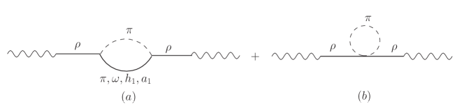
Figure 1: One-loop graphs for the two-point function contributing to self-energy of $\rho$ meson.

In this work we are interested in finding the leading temperature effect modifying the free propagation of the virtual $\rho$ meson at $q^{2}$ below the continuum. At low temperature, the medium is populated mostly by pions. Thus we consider one-loop self-energy graphs of Fig. 1(a), consisting of a pion and another low mass hadron $h$, along with the pion itself. There is a series of such hadronic states with increasing masses. Of course, because of the presence of thermal distribution function, their contributions fall off exponentially with their masses at sufficiently high $q^{2}$. But it is not a priori clear, up to what mass the hadrons should be retained in our low $q^{2}$ calculation. Here we take the particles $h$ to consist of $\omega,h_{1}$ and $a_{1}$, postponing discussion on this point to the last Section. Along with these graphs, we also include the seagull graph of Fig. 1(b), where the loop represents a single pion propagator, those of heavy particles contributing insignificantly at low temperatures that we consider here.

The two-point function in the hadronic phase can be evaluated in chiral perturbation theory by using the method of external fields [13]. Here one introduces (classical) external vector field $v_{\mu}^{i}(x)$ coupled to the vector current $V_{\mu}^{i}(x)$ (and an axial-vector field $a_{\mu}^{i}(x)$ coupled to the axial-vector current $A_{\mu}^{i}(x)$). The resulting terms perturb the original $QCD$ Lagrangian as

$${\cal L}_{QCD}\to{\cal L}_{QCD}+v_{\mu}^{i}V_{i}^{\mu}+a_{\mu}^{i}A_{i}^{\mu}$$ (2.5)

The global chiral symmetry group $SU(2)_{R}\times SU(2)_{L}$ of massless $QCD$ is thus raised to the corresponding local gauge invariance. To arrive at the resulting effective field theory, we have to define the various fields and their covariant derivatives transforming properly under the symmetry group [14, 15, 16, 17]. The Goldstone fields representing the pions may be described by the unitary matrix,

$$U(x)=e^{i\pi(x)/F_{\pi}}~{},~{}~{}~{}~{}~{}~{}~{}~{}\pi(x)=\sum_{i=1}^{3}\pi^{i}(x)\tau^{i}~{}~{},$$ (2.6)

where the constant $F_{\pi}$ can be identified with the pion decay constant, $F_{\pi}=93$ MeV and $\tau^{a}$ are the Pauli matrices. One also defines $u(x)$, such that $u^{2}=U$, because of its transformation rule linking $SU(2)_{R,L}$ to the unbroken group $SU(2)_{V}$. The non-Goldstone iso-triplet field $R_{\mu}(x)$ representing $\rho$ and $a_{1}$ mesons,

$$R_{\mu}(x)=\frac{1}{\sqrt{2}}\sum_{i=1}^{3}\,R_{\mu}^{i}(x)\tau^{i},$$ (2.7)

transforms as

$$R_{\mu}\rightarrow h\,R_{\mu}\,h^{\dagger},~{}~{}~{}~{}h(\pi)\in SU(2)_{V},$$ (2.8)

while the singlet field $S_{\mu}(x)$ representing $\omega$ and $h_{1}$ mesons, of course, remains unchanged. The covariant derivatives of $U$ and $R_{\mu}$ are defined by

$$D_{\mu}U=\partial_{\mu}U-i(v_{\mu}+a_{\mu})U+iU(v_{\mu}-a_{\mu}),$$ (2.9)

and

$$\nabla_{\mu}R_{\nu}=\partial_{\mu}R_{\nu}+[\Gamma_{\mu},R_{\nu}]$$ (2.10)

with the connection

$$\Gamma_{\mu}=\frac{1}{2}\left(u^{\dagger}[\partial_{\mu}-i(v_{\mu}+a_{\mu})]u+u[\partial_{\mu}-i(v_{\mu}-a_{\mu})]u^{\dagger}\frac{}{}\right)$$ (2.11)

Finally we have the usual definition of field strengths $F^{\mu\nu}_{R,L}$ associated with the non-abelian external fields $(v_{\mu}\pm a_{\mu})$, where $v_{\mu}=\sum v_{\mu}^{i}\tau^{i}/2$ and $a_{\mu}=\sum a_{\mu}^{i}\tau^{i}/2$. We can now write the leading term in the effective lagrangian for the Goldstone bosons as

$${\cal{L}}=\frac{F_{\pi}^{2}}{4}\left\{\langle D_{\mu}UD^{\mu}U\rangle+m_{\pi}^{2}\langle U+U^{\dagger}\rangle\right\}$$ (2.12)

It is possible to define new variables related to $D_{\mu}U$ and $F^{\mu\nu}_{R,L}$, namely [16, 17],

$$u_{\mu}=iu^{\dagger}D_{\mu}Uu^{\dagger}=u_{\mu}^{\dagger}$$ (2.13)

and

$$f_{\pm}^{\mu\nu}=\pm u^{\dagger}F_{R}^{\mu\nu}u+uF_{L}^{\mu\nu}u^{\dagger}$$ (2.14)

which transform exactly as $R_{\mu}(x)$ in (2.8). We now have all the variables relevant to non-Goldstone bosons, that transform under $SU(2)_{V}$ only. It is now simple to write the different pieces of the Lagrangian density, that are invariant under $SU(2)_{V}$ and hence also under $SU(2)_{R}\times SU(2)_{L}$. Accordingly, we have the kinetic part as

$${\cal{L}}_{kin}=\sum\left(-\frac{1}{4}\langle R_{\mu\nu}R^{\mu\nu}\rangle+\frac{1}{2}m_{R}^{2}\langle R_{\mu}R^{\mu}\rangle\right)+\sum\left(-\frac{1}{4}S_{\mu\nu}S^{\mu\nu}+\frac{1}{2}m_{S}^{2}S_{\mu}S^{\mu}\right)\,,$$ (2.15)

where

$$R_{\mu\nu}=\nabla_{\mu}R_{\nu}-\nabla_{\nu}R_{\mu},~{}~{}~{}~{}S_{\mu\nu}=\partial_{\mu}S_{\nu}-\partial_{\nu}S_{\mu}.$$ (2.16)

and the two sums run over the iso-triplets and the iso-singlets. Here and below the symbol $\langle A\rangle$ stands for the trace of the 2$\times$2 matrix $A$. The interaction vertices to leading order in powers of derivatives (momenta) and external fields are given by [16, 17, 18]

$${\cal{L}}_{int}=\frac{1}{2\sqrt{2}m_{\rho}}(F_{\rho}\langle\rho_{\mu\nu}f_{+}^{\mu\nu}\rangle++iG_{\rho}\langle\rho_{\mu\nu}[u^{\mu},u^{\nu}]\rangle)+\frac{g_{1}}{\sqrt{2}}\epsilon_{\mu\nu\lambda\sigma}\omega^{\mu}\langle\rho^{\nu\lambda}u^{\sigma}\rangle+\frac{g_{2}}{\sqrt{2}}h_{1}^{\mu}\langle\rho_{\mu\nu}u^{\nu}\rangle+\frac{i}{2}g_{3}\langle\rho^{\mu\nu}[a_{1\,\mu},u_{\nu}]\rangle$$ (2.17)

Each of these interaction terms is typically a series in powers of the derivative of the pion field. Retaining terms to lowest order, we get the interaction vertices as,

$${\cal{L}}^{(1)}_{int} = \frac{F_{\rho}}{m_{\rho}}\partial^{\mu}\vec{v}^{\nu}\cdot(\partial_{\mu}\vec{\rho}_{\nu}-\partial_{\nu}\vec{\rho}_{\mu})$$ (2.18)

$$-\frac{2G_{\rho}}{m_{\rho}F_{\pi}^{2}}\partial_{\mu}\vec{\rho}_{\nu}\cdot\partial^{\mu}\vec{\pi}\times\partial^{\nu}\vec{\pi}$$

$$+\frac{g_{1}}{F_{\pi}}\epsilon_{\mu\nu\lambda\sigma}(\partial^{\nu}\omega^{\mu}\vec{\rho}^{\lambda}-\omega^{\mu}\partial^{\nu}\vec{\rho}^{\lambda})\cdot\partial^{\sigma}\vec{\pi}$$

$$-\frac{g_{2}}{F_{\pi}}h_{1}^{\mu}(\partial_{\mu}\vec{\rho}_{\nu}-\partial_{\nu}\vec{\rho}_{\mu})\cdot\partial^{\nu}\vec{\pi}$$

$$+\frac{g_{3}}{F_{\pi}}(\partial_{\mu}\vec{\rho}_{\nu}-\partial_{\nu}\vec{\rho}_{\mu})\cdot\vec{a}_{1}^{\mu}\times\partial^{\nu}\vec{\pi}$$

The magnitude of the coupling constants may be determined from the observed decay rates of the particles [19]. Thus the decay rate $\Gamma(\rho^{0}\to e^{+}\,e^{-})=6.9$ keV gives $F_{\rho}=154$ MeV. The decay rate $\Gamma(\rho\to 2\pi)=153$ MeV gives $G_{\rho}=69$ MeV. Similarly the decay rates $\Gamma(\omega\to 3\pi)=7.6$ MeV,  $\Gamma(h_{1}\to\rho\pi)\simeq 360$ MeV and $\Gamma(a_{1}\to\rho\pi)\simeq 400$ MeV give respectively $g_{1}=.87,\,g_{2}=1.0$ and $g_{3}=1.1$.

The leading term for the four-point vertex needed in the seagull graph (Fig. 1(b)) arises from the kinetic term for the $\rho$ meson appearing in (2.15),

$${\cal{L}}^{(2)}_{int}=-\frac{1}{8F_{\pi}^{2}}\langle[\rho^{\nu},\partial_{\mu}\rho_{\nu}][\pi,\partial^{\mu}\pi]\rangle$$ (2.19)

We note that this term in the chiral Lagrangian reproduces the famous current algebra result for the leading threshold behaviour of pion scattering off a heavy target, which is $\rho$ in the present case [20].

3 Kinematics

The isospin structure of $T^{ab,ij}_{\mu\nu}$ is clearly given by $\delta^{ij}$, which we omit from now on. We need to analyse its thermal and Lorentz index structures to extract the relevant scalar functions.

We introduce the (four-dimensionally) transverse $\rho$ meson propagator $G_{\mu\nu}^{ab}$ by removing from $T_{\mu\nu}^{ab}$ the factor $K\equiv(F_{\rho}q^{2}/m_{\rho})^{2}$, representing the current-$\rho$ coupling at both ends of graphs of Fig. 1,

$$T_{\mu\nu}^{ab}(q)=KG_{\mu\nu}^{ab}(q)$$ (3.1)

The free elements are

$$T_{\mu\nu}^{(0)ab}(q)=KG_{\mu\nu}^{(0)ab}(q),~{}~{}~{}G_{\mu\nu}^{(0)ab}(q)=\left(-g_{\mu\nu}+\frac{q_{\mu}q_{\nu}}{q^{2}}\right)D^{ab}(q),$$ (3.2)

where $D^{ab}(q)$ is the free thermal propagator of a scalar particle of mass $m_{\rho}$. Comparing with Eq.(A.15), we find that $G_{\mu\nu}^{(0)ab}(q)$ is indeed the (four-dimensionally) transverse part of the free vector propagator $D_{\mu\nu}^{ab}(q)$.

Now $G$ satisfies the familiar Dyson equation,

$$G_{\mu\nu}^{ab}(q)=G_{\mu\nu}^{(0)ab}(q)-G_{\mu\lambda}^{(0)ac}(q)\Pi^{cd,\lambda\sigma}(q)G_{\sigma\nu}^{db}(q)$$ (3.3)

where $\Pi_{\mu\nu}^{ab}(q)$ represents the $\rho$ meson self energy. As shown in the Appendix, we can diagonalise the thermal matrices to get rid of the thermal indices, getting the Dyson equation in terms of the diagonal elements (denoted by a bar) as

$$\overline{G}_{\mu\nu}(q)=\overline{G}_{\mu\nu}^{(0)}(q)-\overline{G}_{\mu\lambda}^{(0)}(q)\overline{\Pi}^{\lambda\sigma}(q)\overline{G}_{\sigma\nu}(q),~{}~{}~{}~{}~{}\overline{G}^{(0)}_{\mu\nu}(q)=\left(-g_{\mu\nu}+\frac{q_{\mu}q_{\nu}}{q^{2}}\right)\frac{-1}{q^{2}-m_{\rho}^{2}+i\epsilon}$$ (3.4)

Here $\overline{\Pi}_{\mu\nu}(q)$ is related to the $11$-component by Eq. (A.18) of the Appendix.

Being free from thermal indices, the Dyson equation may be solved in a way similar to that in vacuum. The vector current conservation leads to

$$q^{\mu}\overline{G}_{\mu\nu}(q)=q^{\nu}\overline{G}_{\mu\nu}(q)=0$$

At finite temperature there are two independent second rank tensors satisfying this condition. To construct them we introduce the four-velocity $u_{\mu}$ of the heat bath (not to be confused with the field $u_{\mu}$ defined in the previous section), even though we shall do explicit calculations in its rest frame $[u^{\mu}=(1,0)]$. We thus have one more scalar variable, $u\cdot q$ in addition to $q^{2}$. Introducing also the transverse variable $\widetilde{u}_{\mu}=u_{\mu}-u\cdot q\,q_{\mu}/q^{2}$, we can build two independent tensors

$$P_{\mu\nu}=-g_{\mu\nu}+\frac{q_{\mu}q_{\nu}}{q^{2}}-\frac{q^{2}}{\overline{q}^{\,2}}\widetilde{u}_{\mu}\widetilde{u}_{\nu},~{}~{}~{}~{}~{}Q_{\mu\nu}=\frac{(q^{2})^{2}}{\overline{q}^{\,2}}\widetilde{u}_{\mu}\widetilde{u}_{\nu},~{}~{}~{}~{}\overline{q}^{\,2}=(u\cdot q)^{2}-q^{2},$$ (3.5)

satisfying the projection properties

$$P\cdot P=-P,~{}~{}~{}~{}~{}Q\cdot Q=-q^{2}Q,~{}~{}~{}~{}~{}P\cdot Q=0$$ (3.6)

While both $P$ and $Q$ are four-dimensionally transverse, $P$ is also 3-dimensionally transverse. In the literature one generally finds the factor $q^{2}$ instead of $(q^{2})^{2}$ in the definition of $Q_{\mu\nu}$. However, at finite temperature dynamical singularity can appear at $q^{2}=0$. The additional factor of $q^{2}$ keeps the kinematic covariant regular at that point.

We now decompose $\overline{G}_{\mu\nu}$ as

$$\overline{G}_{\mu\nu}=P_{\mu\nu}\overline{G}_{t}+Q_{\mu\nu}\overline{G}_{l}$$ (3.7)

One can further show that the self energy tensor $\overline{\Pi}_{\mu\nu}$ is also transverse [21], leading to an identical decomposition,

$$\overline{\Pi}_{\mu\nu}=P_{\mu\nu}\overline{\Pi}_{t}+Q_{\mu\nu}\overline{\Pi}_{l}$$ (3.8)

Inserting these decompositions in the Dyson equation (3.4) we get the solution,

$$\overline{G}_{t}(q)=\frac{-1}{q^{2}-m_{\rho}^{2}-\overline{\Pi}_{t}(q)},~{}~{}~{}~{}~{}\overline{G}_{l}(q)=\frac{1}{q^{2}}\frac{-1}{q^{2}-m_{\rho}^{2}-q^{2}\overline{\Pi}_{l}(q)}$$ (3.9)

The scalar self-energies may be obtained from the tensor one by taking trace over its indices and contracting them with the velocity four vector,

$$\overline{\Pi}_{t}=-\frac{1}{2}(\overline{\Pi}_{\mu}^{\mu}+\frac{q^{2}}{\bar{q}^{2}}\overline{\Pi}_{00}),~{}~{}~{}~{}\overline{\Pi}_{l}=\frac{1}{\bar{q}^{2}}\overline{\Pi}_{00},~{}~{}~{}\overline{\Pi}_{00}\equiv u^{\mu}u^{\nu}\overline{\Pi}_{\mu\nu}$$ (3.10)

Finally we note a kinematic relation between the transverse and the longitudinal components of the propagator at $\vec{q}=0$. As $\vec{q}\to 0$, the kinematic structures $P_{ij}$ and $Q_{ij}$ depend on how the limit is reached. This unphysical dependence is eliminated, if we take

$$\overline{G}_{t}(q_{0},\vec{q}=0)=q_{0}^{2}\,\overline{G}_{l}(q_{0},\vec{q}=0)$$ (3.11)

Clearly a similar relation must also hold between $\overline{\Pi}_{t,l}$, which is already implied by Eqs. (3.9).

4 Evaluation of loop integrals

One-loop graphs were evaluated in the imaginary time formulation by Weldon [6] and subsequently in the real time version by Kobes and Semenoff [12], which we follow to evaluate the graphs at hand. We begin with the general form of the self-energy loop in vacuum with internal lines for pion and a hadron $h$,

$$\Pi_{\mu\nu}(q)=i\int\frac{d^{4}k}{(2\pi)^{4}}N_{\mu\nu}(q,k)\Delta_{\pi}(k)\Delta_{h}(q-k)~{},$$ (4.1)

where $\Delta_{\pi,h}(q)$ are vacuum propagators of scalar particles of mass $m_{\pi}$ and $m_{h}$ respectively. Tensor structures associated with the two vertices and the vector propagator are included in $N_{\mu\nu}$. Introducing the following three gauge invariant (transverse) tensors,

$$A_{\alpha\beta}(q) = -g_{\alpha\beta}+{q_{\alpha}q_{\beta}}/{q^{2}},$$

$$B_{\alpha\beta}(q,k) = q^{2}k_{\alpha}k_{\beta}-q\cdot k(q_{\alpha}k_{\beta}+k_{\alpha}q_{\beta})+(q\cdot k)^{2}g_{\alpha\beta},$$

$$C_{\alpha\beta}(q,k) = q^{4}k_{\alpha}k_{\beta}-q^{2}(q\cdot k)(q_{\alpha}k_{\beta}+k_{\alpha}q_{\beta})+(q\cdot k)^{2}q_{\alpha}q_{\beta}.$$ (4.2)

we get the tensor $N_{\mu\nu}$ for the different graphs of Fig. 1(a) as

$$N_{\mu\nu}^{(\pi)}(q,k) = \left(\frac{2G_{\rho}}{m_{\rho}F_{\pi}^{2}}\right)^{2}C_{\mu\nu}$$

$$N_{\mu\nu}^{(\omega)}(q,k) = -4\left(\frac{g_{1}}{F_{\pi}}\right)^{2}(B_{\mu\nu}+q^{2}k^{2}A_{\mu\nu})$$

$$N_{\mu\nu}^{(h_{1})}(q,k) = -\left(\frac{g_{2}}{F_{\pi}}\right)^{2}(B_{\mu\nu}-\frac{1}{m_{h_{1}}^{2}}C_{\mu\nu})$$

$$N_{\mu\nu}^{(a_{1})}(q,k) = -2\left(\frac{g_{3}}{F_{\pi}}\right)^{2}(B_{\mu\nu}-\frac{1}{m_{a_{1}}^{2}}C_{\mu\nu})$$ (4.3)

At finite temperature the 11-component of the corresponding self-energy matrix is given by

$$\Pi_{\mu\nu}^{11}(q) = i\int\frac{d^{4}k}{(2\pi)^{4}}N_{\mu\nu}(q,k)D_{\pi}^{11}(k)D_{h}^{11}(q-k)$$ (4.4)

$$= i\int\frac{d^{4}k}{(2\pi)^{4}}N_{\mu\nu}(q,k)\Delta_{\pi}(k)\Delta_{h}(q-k)$$

$$-\int\frac{d^{4}k}{(2\pi)^{3}}N_{\mu\nu}(q,k)\{\Delta_{h}(q-k)n(\omega)\delta(k^{2}-m_{\pi}^{2})+\Delta_{\pi}(k)n(\omega^{\prime})\delta((q-k)^{2}-m_{h}^{2})\}$$

$$-i\int\frac{d^{4}k}{(2\pi)^{2}}N_{\mu\nu}(q,k)n(\omega)n(\omega^{\prime})\delta(k^{2}-m_{\pi}^{2})\delta((q-k)^{2}-m_{h}^{2})\,,$$

on inserting the expression for the thermal propagators $D_{\pi,h}^{11}(q)$ as given by (A.8). Here $n$ is the distribution function at temperature $T$ and $\omega$ and $\omega^{\prime}$ are the energies of the pion and the hadron, $\omega=\sqrt{m_{\pi}^{2}+\vec{k}^{2}},\,\,\omega^{\prime}=\sqrt{m_{h}^{2}+(\vec{q}-\vec{k})^{2}}$. Here the first term refers to vacuum. The second and the third terms are medium dependent, containing the distribution function linearly and quadratically respectively. The third term is purely imaginary.

It is simple to evaluate the $k_{0}$ integral of each of the three pieces in (4.4) and read off the imaginary part. Then we get ${\rm Im}\,\overline{\Pi}(q)$ on using (A.18), associated with the time-ordered product. The imaginary part associated with the retarded propagator is also of interest, particularly in writing the dispersion relation for $\overline{\Pi}(q)$. The two imaginary parts are the same, except for a factor of $\epsilon(q_{0})$. Keeping the retarded propagator in mind, we write (5.1) below for ${\rm Im}\,\overline{\Pi}(q)$. For the real part of $\overline{\Pi}(q)$, the medium dependent contribution is obtained from the second term in (4.4),

$${\rm{Re}}\,\overline{\Pi}_{\mu\nu}(q)=\int\frac{d^{3}k}{(2\pi)^{3}} \left\{\frac{n(\omega)}{2\omega}\left(\frac{N_{\mu\nu}(k_{0}=\omega)}{(q_{0}-\omega)^{2}-{\omega^{\prime}}^{2}}+\frac{N_{\mu\nu}(k_{0}=-\omega)}{(q_{0}+\omega)^{2}-{\omega^{\prime}}^{2}}\right)\right.$$ (4.5)

$$\left.+\frac{n(\omega^{\prime})}{2\omega^{\prime}}\left(\frac{N_{\mu\nu}(k_{0}=q_{0}-\omega^{\prime})}{(q_{0}-\omega^{\prime})^{2}-\omega^{2}}+\frac{N_{\mu\nu}(k_{0}=q_{0}+\omega^{\prime})}{(q_{0}+\omega^{\prime})^{2}-\omega^{2}}\right)\right\}$$

where the integrals are principal valued.

The seagull graph (Fig. 1(b)) involves a contraction of two pion fields with a single derivative at the same space-time point that appear in the interaction Lagrangian (2.18). As a result, the thermal components of the resulting self-energy tensor has the form

$$\Pi^{ab}_{\mu\nu}(q)|_{\rm{seagull}}\sim g_{\mu\nu}\int\frac{d^{4}k}{(2\pi)^{4}}q\cdot k\,D^{ab}(k)\,=\,0\,,$$ (4.6)

if we recall that $D^{ab}$ is a function of $\boldsymbol{k}^{2}$ and $k_{0}^{2}$. Thus in chiral perturbation theory, the contribution of each graph of Fig. 1(a) is transverse by itself, without requiring the seagull graph of Fig. 1(b) to do so, the latter being actually zero.

5 Analytic structure

In writing the expression for the imaginary part of the self-energy, we convert the tensors $N_{\mu\nu}$ and $\overline{\Pi}_{\mu\nu}$ into scalars by combining their components as in (3.10). Also, throughout this Section, we omit for brevity, the subscripts $t$ and $l$ of the scalars, as the equations will be valid for both the transverse and the longitudinal components. We thus get

$${\rm Im}\,\overline{\Pi}(q_{0},\vec{q})=-\pi\int\frac{d^{3}\vec{k}}{(2\pi)^{3}4\omega\omega^{\prime}}\times$$

$$[N(k_{0}=\omega)\{(1+n(\omega)+n(\omega^{\prime}))\delta(q_{0}-\omega-\omega^{\prime})-(n(\omega)-n(\omega^{\prime}))\delta(q_{0}-\omega+\omega^{\prime})\}$$

$$+N(k_{0}=-\omega)\{(n(\omega)-n(\omega^{\prime}))\delta(q_{0}+\omega-\omega^{\prime})-(1+n(\omega)+n(\omega^{\prime}))\delta(q_{0}+\omega+\omega^{\prime})\}]$$ (5.1)

We shall label the four terms above by the indices 1, 2, 3 and 4 in the sequence they appear in (5.1). The functions $N_{t,l}$ for different graphs may be obtained from (4.3). Here it suffices to note that these scalar functions depend on scalars built out of the four-vectors, $q_{\mu},\,k_{\mu}$ and $u_{\mu}$, in such a way that they remain invariant under the simultaneous change of sign of $q_{0}$ and $k_{0}$. We thus get the symmetry relations

$${\rm Im}\,\overline{\Pi}_{3}(-q) = -{\rm Im}\,\overline{\Pi}_{2}(q)$$

$${\rm Im}\,\overline{\Pi}_{4}(-q) = -{\rm Im}\,\overline{\Pi}_{1}(q)\,.$$ (5.2)

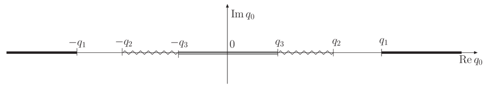
Figure 2: Branch cuts of self-energy function in $q_{0}$ plane for fixed $\vec{q}$ given by $\pi h$ loop. The quantities $q_{1,2,3}$ denote the end points of cuts discussed in the text : $q_{1}=\sqrt{(m_{h}+m_{\pi})^{2}+|\vec{q}|^{2}}$, $q_{2}=\sqrt{(m_{h}-m_{\pi})^{2}+|\vec{q}|^{2}}$ and $q_{3}=|\vec{q}|$. For the $\pi\pi$ loop, $q_{2}$ collapses to $q_{3}$, giving only one variety of Landau cut.

The distribution functions present in different terms of (5.1) may be understood in terms of decay and recombination (inverse decay) probabilities for processes at the vertices of the loop graphs [6]. Denote $n(\omega)$ and $n(\omega^{\prime})$, for short, by $n$ and $n^{\prime}$. Then writing, for example, $1+n+n^{\prime}=(1+n)(1+n^{\prime})-nn^{\prime}$, the first term becomes proportional to the probability for the decay $\rho\rightarrow\pi+h$ with the expected statistical weight $(1+n)(1+n^{\prime})$ for the stimulated emission minus the probability for the inverse decay $\pi+h\rightarrow\rho$ with weight $nn^{\prime}$ for absorption. Similarly, writing $-(n-n^{\prime})=n^{\prime}(1+n)-n(1+n^{\prime})$, the second term gives the probability for $\rho+h\rightarrow\pi$ with weight $n^{\prime}(1+n)$ minus that for $\pi\rightarrow\rho+h$ with weight $n(1+n^{\prime})$.

The regions, in which the four terms of (5.1) are non-vanishing, give rise to cuts in the self-energy function (Fig. 2). These regions are controlled by the respective $\delta$-functions [22]. Thus, the first and the fourth terms are non-vanishing for $q^{2}\geq(m_{h}+m_{\pi})^{2}$, giving the unitary cut, while the second and the third are non-vanishing for $q^{2}\leq(m_{h}-m_{\pi})^{2}$, giving the so-called Landau cut. The origin of these cuts is clear from the discussion in the last paragraph. The unitary cut arises from the states, which can communicate with the $\rho$. These states are, of course, the same as in vacuum, but, as we see above, the probabilities of their occurrence in medium are modified by the distribution functions. Since it is the distribution function for pions and not for heavy mesons that dominates the medium dependent probabilities, the contribution of the unitary cut is referred in the literature as due to modification by the pion cloud in medium [1]. On the other hand, the Landau cut appears only in medium and arises from scattering of $\rho$ with particles present there. We note that this contribution appears as the first term in the virial expansion of the self-energy function [7, 10, 11].

We now come back to evaluate (5.1) explicitly, giving discontinuities of the self-energy function across the cuts in the $q_{0}$ plane for fixed $|\vec{q}|$. We consider a $\pi h$ loop, the $\pi\pi$ loop being a special case. Writing $d^{3}\vec{k}=2\pi\sqrt{\omega^{2}-m_{\pi}^{2}}\,\omega d\omega\,\sin\theta d\theta$, where $\theta$ is the angle between $\vec{q}$ and $\vec{k}$, we can readily integrate over $\cos\theta$ using the $\delta$-functions. But we have to take into account the physical requirement, $|\cos\theta|\leq 1$, which, as we shall see presently, reduces the a priori range ($m_{\pi}$ to $\infty$) of integration over $\omega$. Below we inspect each of the terms of (5.1) and write down explicitly only those pieces that contribute for positive $q_{0}$.

Consider the first two terms of (5.1), for which we have $(q_{0}-\omega)^{2}=\omega^{\prime 2}$, giving

$$\cos\theta=\frac{-R^{2}+2q_{0}\omega}{2|\vec{q}|\sqrt{\omega^{2}-m_{\pi}^{2}}}\,,~{}~{}~{}~{}~{}R^{2}=q^{2}-m_{h}^{2}+m_{\pi}^{2}\,.$$ (5.3)

Then the inequality $|\cos\theta|\leq 1$ becomes

$$q^{2}(\omega-\omega_{+})(\omega-\omega_{-})\leq 0$$ (5.4)

where $\omega_{\pm}$ are the roots of the quadratic equation for $\omega$,

$$\omega_{\pm}=\frac{R^{2}}{2q^{2}}\{q_{0}\pm|\vec{q}|\epsilon(R^{2})v\}\,,~{}~{}~{}v(q^{2})=\sqrt{1-\frac{4q^{2}m_{\pi}^{2}}{R^{4}}}\,.$$ (5.5)

For the first term in (5.1), for which $q^{2}\geq(m_{h}+m_{\pi})^{2}$, as already stated, we have $R^{2}>0$ and $v<1$, so that both $\omega_{+}$ and $\omega_{-}$ have the same sign as that of $q_{0}$. Then this term is non-zero only for positive $q_{0}$ with the integration variable $\omega$ restricted to $\omega_{-}\leq\omega\leq\omega_{+}$. Changing $\omega$ to $x$, $\,\omega=(R^{2}/2q^{2})(q_{0}+|\vec{q}|x)$, we get

$${\rm Im}\,\overline{\Pi}_{1}(q_{0},\vec{q})=-\frac{R^{2}}{32\pi q^{2}}\int_{-v}^{v}dxN(x)\{1+n(\omega)+n(q_{0}-\omega)\}\,,~{}~{}~{}~{}~{}~{}~{}q_{0}\geq\sqrt{(m_{h}+m_{\pi})^{2}+|\vec{q}|^{2}}\,.$$ (5.6)

For the second term in (5.1), we split the region $q^{2}\leq(m_{h}-m_{\pi})^{2}$ into two segments, namely, $0\leq q^{2}\leq(m_{h}-m_{\pi})^{2}$ and $q^{2}\leq 0$ with positive and negative values of $q^{2}$, so that the inequality (5.4) may be applied immediately. Proceeding as before, we find that the first segment leads to a cut in the negative $q_{0}$ region ($-\sqrt{(m_{h}-m_{\pi})^{2}+|\vec{q}|^{2}}\leq q_{0}\leq-|\vec{q}|$) with $\omega$ restricted to $\omega_{-}\leq\omega\leq\omega_{+}$, which we do not write explicitly. The second segment gives a cut in a region over both positive and negative values of $q_{0}$ with $\omega\geq\omega_{-}$, getting

$${\rm Im}\,\overline{\Pi}_{2}(q_{0},\vec{q})=\frac{R^{2}}{32\pi q^{2}}\int_{v}^{\infty}dxN(x)\{n(\omega)-n(\omega-q_{0})\}\,,~{}~{}~{}~{}~{}~{}~{}-|\vec{q}|\leq q_{0}\leq|\vec{q}|\,.$$ (5.7)

The last two terms of (5.1) may be analysed in the same way. Here the expressions for $\cos\theta$ and $\omega_{\pm}$ remains the same as before, except for reversal of sign of $q_{0}$. The position of the cuts in the $q_{0}$ plane are thus obtained from the previous ones by reflecting them at the origin. Thus the third term gives rise to two pieces of imaginary part. With $\widetilde{\omega}=(R^{2}/2q^{2})(-q_{0}+|\vec{q}|x)$, we get

$${\rm Im}\,\overline{\Pi}_{3}(q_{0},\vec{q})=\frac{R^{2}}{32\pi q^{2}}\left\{\begin{array}[]{ll}\displaystyle\int_{-v}^{v}dxN(x)\{n(\widetilde{\omega})-n(q_{0}+\widetilde{\omega})\},&|\vec{q}|\leq q_{0}\leq\sqrt{(m_{h}-m_{\pi})^{2}+|\vec{q}|^{2}}\\ -\displaystyle\int_{v}^{\infty}dxN(x)\{n(\widetilde{\omega})-n(q_{0}+\widetilde{\omega})\},&-|\vec{q}|\leq q_{0}\leq|\vec{q}|\end{array}\right.$$ (5.8)

The fourth term contributes entirely to negative values of $q_{0}$.

The functions $N_{t,l}(x)$ for different graphs are given by (4.3) with the trace and the 00-component of the three tensors calculated from (4.2),

$$A_{\mu}^{\mu}=-3,~{}~{}~{}~{}A_{00}=\frac{|\vec{q}|^{2}}{q^{2}}$$ (5.9)

$$B_{\mu}^{\mu}=m_{\pi}^{2}q^{2}+\frac{R^{4}}{2},~{}~{}~{}~{}B_{00}=-\frac{|\vec{q}|^{2}R^{4}}{4q^{2}}(1-x^{2})$$ (5.10)

$$C_{\mu}^{\mu}=q^{2}(m_{\pi}^{2}q^{2}-\frac{R^{4}}{4}),~{}~{}~{}~{}C_{00}=\frac{|\vec{q}|^{2}R^{4}}{4}x^{2}$$ (5.11)

6 Numerical evaluation

Figure 3: The imaginary and the real parts of self-energy from $\pi\pi$ loop in upper and lower panel respectively. The longitudinal and transverse components are shown separately.

Figure 4: The imaginary and the real parts of self-energy from different $\pi h$ loops in the upper and lower panel respectively. The quantities are averaged over polarisation.

Figure 5: The total imaginary and the real parts of self-energy obtained by summing over $\pi h$ loops in the upper and the lower panel respectively. The longitudinal and the transverse components are shown separately.

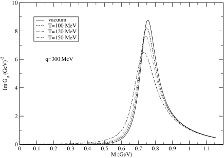
Figure 6: $\rho$ spectral function for different temperatures at fixed three-momentum.

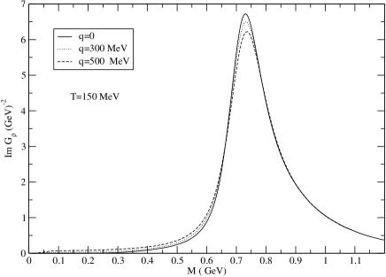
Figure 7: $\rho$ spectral function for different three-momenta at fixed temperature.

We begin with the results of numerical evaluation of the different graphs of Fig. 1(a) for the self-energy of the $\rho$. As usual, we retain the vacuum contribution in the imaginary parts only, assuming the real (divergent) parts to renormalise the $\rho$ meson mass. We calculate the self-energies as a function of $\sqrt{q^{2}}\equiv M$ at fixed values of the three-momentum $\vec{q}$ and temperature $T$. It thus suffices to calculate the self-energies in the time-like region, for positive values of $q_{0}$ starting from $q_{0}=|\vec{q}|$. Then the first part of the Landau cut $(0\leq q_{0}\leq|\vec{q}|)$ cannot appear in our calculation of the imaginary parts.

The $\pi\pi$ loop is distinguished by a large imaginary part of the self-energy, its vacuum part giving $\Gamma_{\rho}\equiv{\rm Im}\,\overline{\Pi}^{(\pi)}/m_{\rho}=153$ MeV at $M=m_{\rho}$. Clearly it is only the unitary cut in the time-like region that gives the imaginary part. The results for this loop are shown in Fig.  3.

In showing the results for other loops, we average their imaginary and real parts over the transverse and longitudinal components,

$$\overline{\Pi}(q)=\frac{1}{3}(q^{2}\overline{\Pi}_{l}(q)+2\overline{\Pi}_{t}(q))$$ (6.1)

They are shown in Fig. 4. Here it is only the second part of the Landau cut $(|\vec{q}|\leq q_{0}\leq\sqrt{(m_{h}-m_{\pi})^{2}+|\vec{q}|^{2}})$, which contributes to the imaginary part. The only exception is the $\pi\omega$ loop, where the unitary cut $(q_{0}\geq\sqrt{(m_{h}+m_{\pi})^{2}+|\vec{q}|^{2}})$ also contributes, its threshold for other loops appearing outside the range of $M$ plotted here. The $\pi\omega$ loop dominates up to about $M\sim 500$ MeV, beyond which the $\pi a_{1}$ loop takes over. The rising trend of the imaginary part at the upper end is due to the contribution of the unitary cut. While the imaginary parts add up, there is appreciable cancellation among the real parts of different loops. Fig. 5 shows separately the behaviour of the transverse and the longitudinal components of both the real and the imaginary parts of self-energy, summed over $\pi h$ loops. Though they differ at low $M$, they tend to converge at higher $M$.

Finally we come to the transverse and the longitudinal components of the spectral function, defined by

$$\mathrm{Im}\,\overline{G}_{t,l}(q)=\frac{-\sum{\rm Im}\,\overline{\Pi}_{t,l}}{(M^{2}-m_{\rho}^{2}-(1,q^{2})\sum\mathrm{Re}\,\overline{\Pi}_{t,l})^{2}+\{(1,q^{2})\sum{\rm Im}\,\overline{\Pi}_{t,l}\}^{2}}$$ (6.2)

where the summation extends over all the loops. Again we take the average over the two components,

$$\mathrm{Im}\,\overline{G}(q)=\frac{1}{3}(q^{2}\mathrm{Im}\,\overline{G}_{l}+2\mathrm{Im}\,\overline{G}_{t})$$ (6.3)

It is drawn in Fig. 6 for three different temperatures at $\vec{q}=300$ MeV, showing a reduction in the height of the peak with the rise of temperature. The pole position, defined by the zero of the real part of of the inverse propagator, shifts from $M=775$ MeV in vacuum to $M=763$ MeV at $T=150$ MeV. Fig. 7 shows this average spectral function for different values of three-momentum $|\vec{q}|$ at $T=150$ MeV. It appears to depend little on the magnitude of $\vec{q}$.

7 Discussion

We present a detailed analysis of the singularities of a one-loop, meson self-energy graph at finite temperature. It is carried out in the real time formulation of field theory in medium. The branch cuts are obtained in the (complex) energy plane at fixed three-momentum. The discontinuities across the cuts are obtained explicitly. The unitary and the Landau cuts arise from what are known in the literature respectively as modifications by pion cloud and in-medium scattering, both effects depending largely on the pion distribution function. The cut structure unifies the discussion of the two parts of the self-energy function.

We also evaluate numerically the self-energy and the resulting spectral function of $\rho$, which may be compared with an earlier determination by Rapp and Gale [9]. Before we do so, however, it would be useful to outline the differences in the two treatments of the problem. Of the series of resonances with increasing masses, which can contribute in the loop calculation, we keep only $\omega,\,h_{1}$ and $a_{1}$, while they include three more. Here we note that although we focus on the $\rho$ meson pole with self-energy corrections, the physical quantity is the complete two-point function, consisting of this pole and the continuum. As we take fewer resonances to calculate the self-energy, we expect the corresponding continuum to begin at a lower value of $q^{2}$ than theirs. The dilepton spectra emitted in the heavy ion collisions depend on the complete two-point function. It would thus be of much interest to work out this emission spectrum with these different evaluations of the two-point function and compare with experiment.

They [9] also include vertex form factors and finite widths of resonances in their evaluation. The form factors go to decrease the contributions from higher momenta. So do the distribution functions for calculations in medium. Thus while the absence of form factors may lead to a significant difference for results in vacuum, it is not so for their medium dependent parts. The finite widths referred to are those of resonances inside a loop integral, where an integration over phase space is involved. In such cases, the results with finite and narrow widths generally differ by no more than, say $10\%$. The case of $\Delta(1237)$ is an example [7]. Also approximating the vector and the axial-vector spectral functions themselves by sharp peaks for $\rho$ and $a_{1}$ in the well-known Weinberg sum rules [23, 24], one commits an error of only a few percent [25].

Finally there is some difference at the level of basic formulae. Their expression for the real part of the self-energy due to singularities in the $q_{0}\leq 0$ region differs from ours (4.5)), even though the difference is numerically small. Also the structure of some of the interaction Lagrangians are different, but again it would not affect the results significantly in the neighbourhood of $M=m_{\rho}$.

Keeping all these differences in mind, we may expect the results of our calculation to agree with that of ref. [9] to within, say $20\%$. Indeed, the imaginary parts agree well within this expectation in a wide region in $M$ around the $\rho$ meson mass. At higher values of $M$, however, our calculation shows a substantial increase due to the inclusion of the unitary cut of the $\pi\omega$ loop.

To conclude, we derive the discontinuities across all the cuts of a self-energy loop of a vector meson. In the literature [9] the self-energy is constructed from the unitary cut of the $\pi\pi$ loop and the Landau cut of different $\pi h$ loops. By contrast, we find that the unitary cut of at least some of the $\pi h$ loops (here $\pi\omega$) may also contribute significantly.

Appendix : Real time field theory at finite temperature

In this Appendix we review briefly the real time formulation of thermal field theory. We construct scalar and vector propagators and diagonalise them, showing that such matrices are actually given by a single analytic function, coinciding essentially with the corresponding result from the imaginary time formulation. But the real time procedure requires neither the frequency sum to evaluate the loop integrals, nor any analytic continuation to physical energies.

Free scalar propagator

First consider the (free) propagator for the scalar field $\phi(x)$,

$$D(\tau,\tau^{\prime};\vec{x}-\vec{x}^{\prime})=i\langle T_{c}\phi(\tau,\vec{x})\phi(\tau^{\prime},\vec{x}^{\prime})\rangle\,.$$ (A.1)

where $x^{\mu}=(\tau,\vec{x})$. Here $\tau$ and $\tau^{\prime}$ are any two points on a contour in the plane of the complex time variable. The contour begins at $-T$ say on the real axis and ends at $-T-i\beta$, nowhere moving upwards and remaining entirely within the analyticity domain $-\beta\leq{\rm Im}(\tau-\tau^{\prime})\leq 0$ [26]. Apart from these restrictions we keep the form of the contour arbitrary at this stage. The delta- and theta- functions on the contour will be denoted by the subscript $c$.

The thermal propagator satisfies the same differential equation as the one in vacuum,

$$(\Box_{c}+m^{2})D(\tau,\tau^{\prime};\vec{x}-\vec{x}^{\prime})=\delta_{c}(\tau-\tau^{\prime})\delta^{3}(\vec{x}-\vec{x}^{\prime}),$$ (A.2)

but obeys a different, thermal boundary condition. If we write

$$D(\tau,\tau^{\prime};\vec{x}-\vec{x}^{\prime})=\theta_{c}(\tau-\tau^{\prime})D^{+}(\tau,\tau^{\prime};\vec{x}-\vec{x}^{\prime})+\theta_{c}(\tau^{\prime}-\tau)D^{-}(\tau,\tau^{\prime};\vec{x}-\vec{x}^{\prime}),$$ (A.3)

and use translation in $\tau$ and cyclicity of the trace in either of $D^{\pm}$, we get the so-called KMS boundary condition as,

$$D^{-}(\tau,\tau^{\prime};\vec{x}-\vec{x}^{\prime})=D^{+}(\tau-i\beta,\tau^{\prime};\vec{x}-\vec{x}^{\prime})$$ (A.4)

To obtain the solution it is convenient to take the spatial Fourier transform,

$$D(\tau,\tau^{\prime};\vec{x}-\vec{x}^{\prime})=\int\frac{d^{3}k}{(2\pi)^{3}}e^{i\vec{k}\cdot(\vec{x}-\vec{x}^{\prime})}D(\tau,\tau^{\prime};\vec{k})$$ (A.5)

The $\tau$-dependence is then given by

$$\left(\frac{d^{2}}{d\tau^{2}}+\omega^{2}\right)D(\tau,\tau^{\prime};\vec{k})=\delta_{c}(\tau-\tau^{\prime})~{}~{}~{}~{}~{}~{}~{}\omega=\sqrt{\vec{k}^{2}+m^{2}}$$ (A.6)

It is now an elementary exercise in Green’s function to solve Eq.(A.6) with the boundary condition (A.4),

$$D(\tau-\tau^{\prime},\vec{k})=\frac{i}{2\omega}\left[e^{-i\omega(\tau-\tau^{\prime})}\{\theta_{c}(\tau-\tau^{\prime})+n(\omega)\}+e^{i\omega(\tau-\tau^{\prime})}\{\theta_{c}(\tau^{\prime}-\tau)+n(\omega)\}\right],$$ (A.7)

where $n(\omega)=\dfrac{1}{e^{\beta\omega}-1}$, getting the particle number distribution function in the propagator.

Figure 8: Contour in time plane for real time formalism

.

Of the variety of possible contours in the complex time plane [27], two are specially interesting, namely the closed one [28] and the symmetrical one [29]. We now choose the latter contour (Fig. 8) with $T\to\infty$, when $D(\tau-\tau^{\prime},\vec{k})$ reduces effectively to four components, which may be assembled in the form of a $2\times 2$ matrix. The Fourier transform $D^{ab}(k)$ of these components can be defined with respect to real time to give [29, 30, 31, 32],

$$D^{11}=-(D^{22})^{*}=\Delta(k)+2\pi in\delta(k^{2}-m^{2})$$

$$D^{12}=D^{21}=2\pi i\sqrt{n(1+n)}\delta(k^{2}-m^{2})$$ (A.8)

where $\Delta(k)$ is the Feynman propagator in vacuum,

$$\Delta(k^{2})=\frac{-1}{k^{2}-m^{2}+i\epsilon}$$ (A.9)

The thermal propagator may be diagonalised in the form

$$D^{ab}(k_{0},\vec{k})=U^{ac}(k_{0})[{\rm diag}\{\Delta(k_{0},\vec{k}),-\Delta^{*}(k_{0},\vec{k})\}]^{cd}U^{db}(k_{0})$$ (A.10)

with the elements of the diagonalising matrix as

$$U^{11}=U^{22}=\sqrt{1+n},~{}~{}~{}U^{12}=U^{21}=\sqrt{n}$$

Writing spectral representations, one can show that $U$ diagonalises not only the free propagator, but also the complete one [12, 18].

Free vector propagator

The thermal propagator for a massive, spin-one particle may be derived in a similar way. Denoting its field by $\rho_{\mu}(x)$, it has the propagator

$$D_{\mu\nu}(\tau,\tau^{\prime};\vec{x}-\vec{x}^{\prime})=i\langle T_{c}\rho_{\mu}(\tau,\vec{x})\rho_{\nu}(\tau^{\prime},\vec{x}^{\prime})\rangle\,.$$ (A.11)

satisfying the differential equation

$$[-g_{\mu\nu}(\Box_{c}+m^{2})+\partial_{\mu}\partial_{\nu}]D^{\nu\rho}(\tau,\tau^{\prime};\vec{x}-\vec{x}^{\prime})=g_{\mu}^{\rho}\delta_{c}(\tau-\tau^{\prime})\delta^{3}(\vec{x}-\vec{x}^{\prime})$$ (A.12)

The thermal boundary condition is again given by an equation similar to that of Eq.(A.4). As before we take the spatial Fourier transform, when the the tensor components satisfy

$$\omega^{2}D^{00}(\tau-\tau^{\prime},\vec{k})+ik_{l}\frac{d}{d\tau}D^{l0}(\tau-\tau^{\prime},\vec{k})=-\delta(\tau-\tau^{\prime})$$

$$\omega^{2}D^{0i}(\tau-\tau^{\prime},\vec{k})+ik_{l}\frac{d}{d\tau}D^{li}(\tau-\tau^{\prime},\vec{k})=0$$

$$-\left[g_{il}\left(\frac{d^{2}}{d\tau^{2}}+\omega^{2}\right)+k_{i}k_{l}\right]D^{lj}(\tau-\tau^{\prime},\vec{k})-ik_{i}\frac{d}{d\tau}D^{0j}=g_{i}^{j}\delta(\tau-\tau^{\prime})$$ (A.13)

It is easy to check that these equations as well as the boundary condition is solved by

$$D_{ij}(\tau-\tau^{\prime},\vec{k}) = -\left(g_{ij}-\frac{k_{i}k_{j}}{m^{2}}\right)D(\tau-\tau^{\prime},\vec{k})$$

$$D_{0i}(\tau-\tau^{\prime},\vec{k}) = i\frac{k_{0}}{m^{2}}\frac{d}{d\tau}D(\tau-\tau^{\prime},\vec{k})$$

$$D_{00}(\tau-\tau^{\prime},\vec{k}) = -\left(1+\frac{1}{m^{2}}\frac{d^{2}}{d\tau^{2}}\right)D(\tau-\tau^{\prime},\vec{k})$$ (A.14)

where $D$ satisfies the same Eq. (A.6) as for the scalar field. We now take the temporal Fourier transform as before and assemble the resulting four dimensional Fourier Transform of the four components of the thermal vector propagator in terms of that for the scalar propagator

$$D_{\mu\nu}^{ab}(k)=\left(-g_{\mu\nu}+\frac{k_{\mu}k_{\nu}}{m^{2}}\right)D^{ab}(k)$$ (A.15)

the Lorentz structure remaining the same as for the vacuum propagator.

Diagonalisation of complete vector propagator

We now turn to Dyson equation (3.3) in the text. As already stated above, both the free and the complete propagator can be diagonalised by the same thermal matrix $U$ ; thus

$$G^{ab}_{\mu\nu}(k_{0},\vec{k})=U^{ac}(k_{0})[{\rm diag}\{\overline{G}_{\mu\nu}(k_{0},\vec{k}),\,-\overline{G}^{*}_{\mu\nu}(k_{0},\vec{k})\}]^{cd}U^{db}(k_{0})$$ (A.16)

As a consequence, the matrix $\Pi^{ab}_{\mu\nu}$ is also diagonalisable by $(U^{-1})^{ab}$,

$$\Pi^{ab}_{\mu\nu}(q)=[U^{-1}(q_{0})]^{ac}[{\rm diag}\{\overline{\Pi}_{\mu\nu}(q),-\overline{\Pi}_{\mu\nu}^{*}(q)\}]^{cd}[U^{-1}(q_{0})]^{db}$$ (A.17)

We thus get the Dyson equation (3.4) in the text for the barred quantities, that are free from the thermal indices. The diagonalised tensor $\overline{\Pi}_{\mu\nu}$ can be related to any of the components of the corresponding matrix. For example, it is related to the $11$ component as

$${\rm Re}\,\overline{\Pi}_{\mu\nu} = {\rm Re}\,\Pi_{\mu\nu}^{11}$$

$${\rm Im}\,\overline{\Pi}_{\mu\nu} = \tanh(\beta\omega/2){\rm Im}\,\Pi_{\mu\nu}^{11}$$ (A.18)

References

[1] R. Rapp and J. Wambach, Adv. Nucl. Phys. 25, 1 (2000)
[2] J. Alam, S. Sarkar, P. Roy, T. Hatsuda and B. Sinha, Ann. Phys.
286, 159 (2000).
[3] R. Arnaldi, et al (NA60 Collaboration), Eur. Phys. J. C61,
711 (2009).
[4] C. Gale and J. I. Kapusta Nucl. Phys. B357, 65 (1991)
[5] K. Haglin, Nucl. Phys. A 584, 719 (1995)
[6] H.A. Weldon, Phys. Rev. D 28, 2007 (1983)
[7] H. Leutwyler and A. Smilga, Nucl. Phys.B 342, 302 (1990)
[8] V.L. Eletsky, M. Belkacem, P.J. Ellis and J.I. Kapusta, Phys.
Rev. C64 035202 (2001).
[9] R. Rapp and C. Gale, Phys. Rev. C 60, 024903 (1999)
[10] S. Jeon and P.J. Ellis, Phys. Rev. D 58, 045013 (1998)