Charge and Current Sum Rules in Quantum Media Coupled to Radiation II

Abstract

This paper is a continuation of the previous study [Šamaj, L.: J. Stat. Phys. 137, 1-17 (2009)], where a sequence of sum rules for the equilibrium charge and current density correlation functions in an infinite (bulk) quantum media coupled to the radiation was derived by using Rytov’s fluctuational electrodynamics. Here, we extend the previous results to inhomogeneous situations, in particular to the three-dimensional interface geometry of two joint semi-infinite media. The sum rules derived for the charge-charge density correlations represent a generalization of the previous ones, related to the interface dipole moment and to the long-ranged tail of the surface charge density correlation function along the interface of a conductor in contact with an inert (not fluctuating) dielectric wall, to two fluctuating semi-infinite media of any kind. The charge-current and current-current sum rules obtained here are, to our knowledge, new. The current-current sum rules indicate a breaking of the directional invariance of the diagonal current-current correlations by the interface. The sum rules are expressed explicitly in the classical high-temperature limit (the static case) and for the jellium model (the time-dependent case).

1 Introduction

The models studied in this paper are composed of spinless charged particles, classical or quantum, which are non-relativistic, i.e. they behave according to Schrödinger and not Dirac. On the other hand, the interaction of charged particles via the radiated electromagnetic (EM) field can be considered either non-relativistic (nonretarded) or relativistic (retarded). In the nonretarded regime, magnetic forces are ignored by taking the speed of light $c\to\infty$, so that the particles interact only via instantaneous Coulomb potentials. In the retarded regime, $c$ is assumed finite and the particles are fully coupled to both electric (longitudinal) and magnetic (transverse) parts of the radiated field.

One of the tasks in the equilibrium statistical mechanics of charged systems is to determine how fluctuations of microscopic quantities like charge and current densities, induced electric and magnetic fields, etc., around their mean values are correlated in time and space. A special attention is devoted to the asymptotic large-distance behavior of the correlation functions and to the sum rules, which fix the values of certain moments of the correlation functions.

Two complementary types of approaches exist in the theory of charged systems. The microscopic approaches, based on the explicit solution of models defined by their microscopic Hamiltonians, are usually restricted to the nonretarded regime. A series of sum rules for the charge and current correlation functions has been obtained for infinite (bulk), semi-infinite and fully finite geometries (see review Martin88 ). The quantum sum rules are available only for the jellium model of conductors (sometimes called the one-component plasma), i.e. the system of identically charged pointlike particles immersed in a neutralizing homogeneous background, in which there is no viscous damping of the long-wavelength plasma oscillations. The macroscopic approaches are based on the assumption of validity of macroscopic electrodynamics. Being essentially of mean-field type, they are expected to provide reliable results only for the leading terms in the asymptotic long-wavelength behavior of correlations. In general, these approaches are able to predict basic features of physical systems also in the retarded regime. A macroscopic theory of equilibrium thermal fluctuations of the EM field in quantum media, conductors and dielectrics, was proposed by Rytov Rytov53 ; Levin67 ; LP .

In a recent work Samaj09 , a sequence of static or time-dependent sum rules, known or new, was obtained for the bulk charge and current density correlation functions in quantum media fully coupled to the radiation by using Rytov’s fluctuational electrodynamics. A technique was developed to extract the classical and purely quantum-mechanical parts of these sum rules. The sum rules were critically tested on the jellium model. A comparison was made with microscopic approaches to systems of particles interacting through Coulomb forces only Martin85 ; John93 ; in contrast to microscopic results, the current-current density correlation function was found to be integrable in space, in both classical and quantum cases.

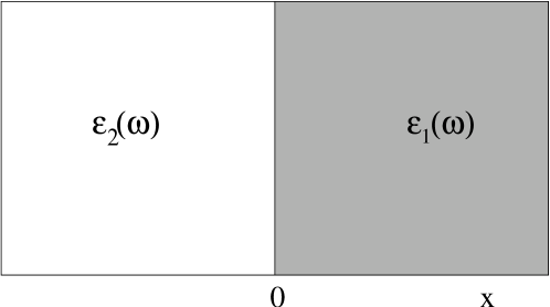
Figure 1: Two semi-infinite media characterized by dielectric functions $\epsilon_{1}(\omega)$ and $\epsilon_{2}(\omega)$

This paper is a continuation of the previous study Samaj09 . It aims at generalizing the previous sum rules to inhomogeneous situations, in particular to the interface geometry of two semi-infinite media with different dielectric functions pictured in Fig. 1. It should be emphasized that this is not exactly the configuration considered in some previous studies. The standard configuration was a conductor in contact with an “inert” (not fluctuating) wall of the static dielectric constant $\epsilon_{W}$. The presence of a dielectric wall is reflected itself only via the introduction of charge images; the microscopic quantities inside the inert wall do not fluctuate, they are simply fixed to their mean values. Such a mathematical model can provide a deformed description of real materials and, as is shown in this paper, it really does. The only exception from the described inert-wall systems is represented by the specific (two-dimensional) two-densities jellium, i.e. the interface model of two joint semi-infinite jelliums with different mean particle densities, treated in Blum84 ; Jancovici84 ; Alastuey84 . It stands to reason that in the case of the vacuum $(\epsilon_{W}=1)$ plain hard wall, there is no charge which could fluctuate and the inert-wall model is therefore adequate.

To our knowledge, the sum rules for a (fluctuating) conductor medium in contact with a dielectric (inert) wall obtained up to now were restricted to the charge-charge density correlation functions. The inhomogeneous charge-charge sum rules are either of dipole type or they are related to the long-ranged decay of the surface charge correlation function along the interface.

The classical dipole sum rule for the static charge-charge density correlations follows directly from the Carnie and Chan generalization to nonuniform fluids of the second-moment Stillinger-Lovett condition Carnie81 ; Carnie83 . The time-dependent classical dipole sum rule was derived in Lebowitz85 . A time-dependent generalization of the Carnie-Chan rule to the quantum (nonretarded) jellium and the consequent derivation of the quantum dipole sum rule for the time-dependent charge-charge density correlations were accomplished in Ref. Jancovici85b .

The bulk charge correlation functions exhibit a short-ranged, usually exponential, decay in classical conductors due to the screening. On the other hand, for a semi-infinite conductor in contact with a vacuum or (inert) dielectric wall, the correlation functions of the surface charge density on the conductor decay as the inverse cube of the distance at asymptotically large distances Usenko79 . In the classical static case, this long-range phenomenon has been obtained microscopically Jancovici82a ; Jancovici82b as well as by using simple macroscopic argument based on the electrostatic method of images Jancovici95 ; the prefactor to the asymptotic decay was found to be universal, i.e. independent of the composition of the Coulomb fluid. In the quantum case of the specific jellium model, ignoring retardation effects, a nonuniversal prefactor to the asymptotic decay was obtained, for both static Jancovici85a and time-dependent Jancovici85b ; Jancovici85a correlation functions. Recently Samaj08 ; Jancovici09a , by using the inhomogeneous version of Rytov’s fluctuational theory, we have extended the quantum analysis of the jellium to the retarded case. We got a surprising result: for both static and time-dependent surface charge correlation functions, the inclusion of retardation effects causes the quantum prefactor to take its universal static classical form, for any temperature. The restoration of the classical prefactor by retardation effects was observed subsequently for arbitrary (conductor, dielectric, vacuum) configurations of two semi-infinite quantum media Jancovici09b .

In this paper, we apply the inhomogeneous version of the Rytov fluctuational theory to extend the bulk sum rules, derived in Samaj09 , to the geometry of two joint semi-infinite media with distinct dielectric functions in Fig. 1. The sum rules derived for the charge-charge density correlations represent a generalization of the previous (dipole moment and surface charge) ones, valid for a conductor system in contact with an inert dielectric wall, to two fluctuating semi-infinite media of any kind. The fundamental differences between the results for the inert and fluctuating wall descriptions are pointed out. The charge-current and current-current sum rules obtained here are, to our knowledge, new. The current-current sum rules indicate a breaking of the directional invariance of the diagonal current-current correlations by the interface. The sum rules are expressed explicitly in the classical high-temperature limit (the static case) and for the jellium model (the time-dependent case).

The paper is organized as follows. In Sec. 2, we review the inhomogeneous Rytov theory of EM field fluctuations and write down basic expressions for the charge and current densities; explicit results for the elements of the retarded Green function tensor for the two semi-infinite media configuration in Fig.1 are presented in Appendix. Dipole sum rules for the charge-charge density correlation functions are derived in Sect. 3. The sum rules related to the long-ranged tail of the surface charge density correlation function along the interface between two media are discussed in Sect. 4 which is divided into three parts. In the first part 4.1, we generalize the classical static analysis of a medium in vacuum Jancovici09b to arbitrary media configurations. Part 4.2 concerns the derivation of a classical static relation between the dipole moment and the large distance asymptotic of the surface charge density. Part 4.3 is a brief recapitulation of the quantum case, in both retarded and nonretarded regimes. The sum rules for the charge-current and current-current density correlation functions are the subject of Sects. 5 and 6, respectively. Section 7 is the Conclusion.

2 Fluctuational Formalism

We consider the (3+1)-dimensional space of points, defined by Euclidean vectors ${\bf r}=(x,y,z)$ and time $t$. We shall deal with semi-infinite geometries, inhomogeneous say along the first coordinate $x$; it is useful to denote the remaining two coordinates normal to $x$ as ${\bf R}=(y,z)$. The model consists in two distinct semi-infinite media (conductors, dielectrics or vacuum) with the frequency-dependent dielectric functions $\epsilon_{1}(\omega)$ and $\epsilon_{2}(\omega)$ which are localized in the complementary half spaces $\Lambda_{1}=\{{\bf r}=(x>0,{\bf R})\}$ and $\Lambda_{2}=\{{\bf r}=(x<0,{\bf R})\}$, respectively, so that the interface between the media is localized at $x=0$ (see Fig. 1). We shall assume that the media have no magnetic structure, i.e. they are not magnetoactive, and the magnetic permeabilities $\mu_{1}=\mu_{2}=1$. The two-point functions studied in this paper will be translationally invariant in time and in the vector space ${\bf R}$ perpendicular to the $x$ axis, and so we shall use the (partial) Fourier representation

$$f(t,{\bf r};t^{\prime},{\bf r}^{\prime}) \equiv f(t-t^{\prime},{\bf R}-{\bf R}^{\prime};x,x^{\prime})$$ (2.1)

$$= \int_{-\infty}^{\infty}\frac{{\rm d}\omega}{2\pi}\int_{R^{2}}\frac{{\rm d}{\bf q}}{(2\pi)^{2}}{\rm e}^{-{\rm i}\omega(t-t^{\prime})+{\rm i}{\bf q}\cdot({\bf R}-{\bf R}^{\prime})}f(\omega,{\bf q};x,x^{\prime}),$$

where $\omega$ denotes the frequency and ${\bf q}=(q_{y},q_{z})$ is the two-dimensional wave vector.

The induced EM fields inside a material medium are random variables which fluctuate in time and space due to the random motion of charged particles. In the long-wavelength scale, the EM fluctuations are described by the Rytov theory Rytov53 ; Levin67 ; LP . This theory is usually formulated in the Weyl gauge with the scalar potential $\phi(t,{\bf r})=0$, so that the (classical) vector potential ${\bf A}(t,{\bf r})$ with components $A_{j}(t,{\bf r})$ $(j=x,y,z)$ determines the microscopic electric and magnetic fields as follows

$${\bf E}=-\frac{1}{c}\frac{\partial{\bf A}}{\partial t},\qquad{\bf B}={\rm curl}{\bf A}$$ (2.2)

(we use Gaussian units), where $c$ is the speed of light. In the context of the quantized EM field theory, the crucial role is played by the retarded photon Green function tensor $\mathsf{D}$ defined by

$${\rm i}D_{jk}(t-t^{\prime};{\bf r},{\bf r}^{\prime})=\left\{\begin{array}[]{lr}\langle A_{j}(t,{\bf r})A_{k}(t^{\prime},{\bf r}^{\prime})-A_{k}(t^{\prime},{\bf r}^{\prime})A_{j}(t,{\bf r})\rangle,&t\geq t^{\prime},\cr&\cr 0,&t<t^{\prime},\end{array}\right.$$ (2.3)

where $A_{j}(t,{\bf r})$ denotes the vector-potential operator in the Heisenberg picture and the angular brackets represent the equilibrium averaging at temperature $T$, or the inverse temperature $\beta=1/(k_{\rm B}T)$. For non-magnetoactive media, the Green function tensor possesses the symmetry

$$D_{jk}(t-t^{\prime};{\bf r},{\bf r}^{\prime})=D_{kj}(t-t^{\prime};{\bf r}^{\prime},{\bf r}).$$ (2.4)

In the Fourier space, the symmetry is expressible as

$$D_{jk}(\omega,{\bf q};x,x^{\prime})=D_{kj}(\omega,-{\bf q};x^{\prime},x).$$ (2.5)

The validity of macroscopic Maxwell’s equations for the mean values of the EM fields implies, in the frequency Fourier space, a set of differential equations of dyadic type fulfilled by the Green function tensor:

$$\sum_{l}\left[\frac{\partial^{2}}{\partial x_{j}\partial x_{l}}-\delta_{jl}\Delta-\delta_{jl}\frac{\omega^{2}}{c^{2}}\epsilon(\omega,{\bf r})\right]D_{lk}(\omega;{\bf r},{\bf r}^{\prime})=-4\pi\hbar\delta_{jk}\delta({\bf r}-{\bf r}^{\prime}).$$ (2.6)

Here, in order to simplify the notation, the vector ${\bf r}=(x,y,z)$ is represented as $(x_{1},x_{2},x_{3})$. The source point ${\bf r}^{\prime}$ and the index $k$ only act as some fixed parameters, the boundary conditions are with respect to the field point ${\bf r}$. There is an obvious boundary condition of regularity $D_{jk}(\omega;{\bf r},{\bf r}^{\prime})\to 0$ for asymptotically large distances $|{\bf r}-{\bf r}^{\prime}|\to\infty$. At an interface between two different media, the boundary conditions correspond to the macroscopic requirement that the tangential components of the fields ${\bf E}$ and ${\bf H}={\bf B}$, considered in the gauge (2.2), be continuous. The Green function tensor for the geometry pictured in Fig. 1 was obtained in a number of papers, see e.g. the method using vector wave functions Li94 or the Weyl expansion method Tomas95 ; Dung98 . The results are usually written in a complicated way, by using the dyadic notation for the tensors. In order to enable the reader to reproduce easily calculations performed in this work, in the Appendix we present explicitly the Fourier transforms (2.1) of the tensor elements $D_{jk}(\omega,{\bf q};x,x^{\prime})$ for two possible cases: the points ${\bf r}$ and ${\bf r}^{\prime}$ are in the same half space or they are in different half spaces.

Applying the fluctuation-dissipation theorem and assuming the symmetry (2.5), the fluctuations of the vector potential are described by the formula

$$\langle A_{j}(\omega,{\bf q};x)A_{k}(-\omega,-{\bf q};x^{\prime})\rangle^{s}=-\coth\left(\frac{\beta\hbar\omega}{2}\right){\rm Im}\,D_{jk}(\omega,{\bf q};x,x^{\prime}),$$ (2.7)

where Im means the imaginary part and $\langle A_{j}(\omega,{\bf q};x)A_{k}(-\omega,-{\bf q};x^{\prime})\rangle^{s}$ is the Fourier transform of the symmetrized correlation function

$$\langle A_{j}(t,{\bf r})A_{k}(t^{\prime},{\bf r}^{\prime})\rangle^{s}\equiv\frac{1}{2}\langle A_{j}(t,{\bf r})A_{k}(t^{\prime},{\bf r}^{\prime})+A_{k}(t^{\prime},{\bf r}^{\prime})A_{j}(t,{\bf r})\rangle^{\rm T}.$$ (2.8)

Here, $\langle\cdots\rangle^{\rm T}$ represents a truncated equilibrium average, $\langle AB\rangle^{\rm T}=\langle AB\rangle-\langle A\rangle\langle B\rangle$.

The relation (2.7) enables us to calculate the symmetrized two-point correlation function of arbitrary statistical quantities. Let a scalar quantity $u$ be expressible in terms of the components of the vector potential, in the classical format and in the gauge (2.2), as $u(t,{\bf r})=\sum_{j}{\bf U}_{j}A_{j}(t,{\bf r})$, where $\{{\bf U}_{j}\}$ $(j=x,y,z)$ are operators acting on time and space variables. Within the spectral representation with a single frequency $\omega$ and two-dimensional vector ${\bf q}$, $f(t,{\bf r})={\rm e}^{-{\rm i}\omega t+{\rm i}{\bf q}\cdot{\bf R}}f(\omega,{\bf q};x)$, this relation takes a partially algebraic form $u(\omega,{\bf q};x)=\sum_{j}{\bf U}_{j}(\omega,{\bf q};x)A_{j}(\omega,{\bf q};x)$ (${\bf U}_{j}$ can still act as operators on the $x$ coordinate). It follows from the definition (2.1) that the Fourier transform of the symmetrized two-point correlation function of statistical quantities $u$ and $v$, $\langle u(t,{\bf r})v(t^{\prime},{\bf r}^{\prime})\rangle^{s}$, is then determined by

$$\langle u(x)v(x^{\prime})\rangle^{s}_{\omega,{\bf q}} \equiv \langle u(\omega,{\bf q},x)v(-\omega,-{\bf q},x^{\prime})\rangle^{s}$$ (2.9)

$$= \sum_{jk}{\bf U}_{j}(\omega,{\bf q};x){\bf V}_{k}(-\omega,-{\bf q};x^{\prime})\langle A_{j}(x)A_{k}(x^{\prime})\rangle^{s}_{\omega,{\bf q}},$$

where $\langle A_{j}(x)A_{k}(x^{\prime})\rangle^{s}_{\omega,{\bf q}}\equiv\langle A_{j}(\omega,{\bf q};x)A_{k}(-\omega,-{\bf q};x^{\prime})\rangle^{s}$ is given by (2.7). The statistical quantities of our interest are the volume charge density $\rho$ and the electric current density ${\bf j}$. The charge density, defined by $4\pi\rho(t,{\bf r})={\rm div}\,{\bf E}$, is expressible in terms of the vector potential components as follows

$$\rho(\omega,{\bf q};x)=\frac{\omega}{4\pi c}\left({\rm i}\frac{\partial}{\partial x}A_{x}-q_{y}A_{y}-q_{z}A_{z}\right),$$ (2.10)

where the abbreviated notation $A_{j}\equiv A_{j}(\omega,{\bf q};x)$ is used. The vector components of the electric current density, defined by $4\pi{\bf j}(t,{\bf r})=c\ {\rm curl}\,{\bf B}-\partial_{t}{\bf E}$, are expressible as

$$j_{x}(\omega,{\bf q};x) = \frac{c}{4\pi}\left[\left(q^{2}-\frac{\omega^{2}}{c^{2}}\right)A_{x}-{\rm i}\frac{\partial}{\partial x}\left(q_{y}A_{y}+q_{z}A_{z}\right)\right],$$ (2.11)

$$j_{y}(\omega,{\bf q};x) = \frac{c}{4\pi}\left[-{\rm i}q_{y}\frac{\partial}{\partial x}A_{x}+\left(q_{z}^{2}-\frac{\omega^{2}}{c^{2}}-\frac{\partial^{2}}{\partial x^{2}}\right)A_{y}-q_{y}q_{z}A_{z}\right],\phantom{eee}$$ (2.12)

$$j_{z}(\omega,{\bf q};x) = \frac{c}{4\pi}\left[-{\rm i}q_{z}\frac{\partial}{\partial x}A_{x}-q_{y}q_{z}A_{y}+\left(q_{y}^{2}-\frac{\omega^{2}}{c^{2}}-\frac{\partial^{2}}{\partial x^{2}}\right)A_{z}\right].\phantom{eee}$$ (2.13)

3 Dipole sum rules

In the present and subsequent sections, we treat the symmetrized charge-charge density correlation function $\langle\rho(t,{\bf r})\rho(0,{\bf r}^{\prime})\rangle^{s}$, where we set $t^{\prime}=0$ for simplicity. This function fulfills the obvious neutrality condition

$$\int{\rm d}{\bf r}\langle\rho(t,{\bf r})\rho(0,{\bf r}^{\prime})\rangle^{s}=\int{\rm d}{\bf r}^{\prime}\langle\rho(t,{\bf r})\rho(0,{\bf r}^{\prime})\rangle^{s}=0.$$ (3.1)

Let us consider a (partial) dipole moment carried by the charge-charge density correlation function $\langle\rho(t,{\bf r})\rho(0,{\bf r}^{\prime})\rangle^{s}$, with the point ${\bf r}$ being constrained to the region $\Lambda_{1}$:

$$D^{(1)}(t)=\int_{-\infty}^{\infty}{\rm d}x^{\prime}\int_{0}^{\infty}{\rm d}x\int{\rm d}{\bf R}\,x\langle\rho(t,{\bf r})\rho(0,{\bf r}^{\prime})\rangle^{s}.$$ (3.2)

Note that, due to the translational invariance of the correlation function in the space perpendicular to the $x$ axis, the integration $\int{\rm d}{\bf R}$ can be equivalently rewritten as $\int{\rm d}{\bf R}^{\prime}$ or $\int{\rm d}({\bf R}-{\bf R}^{\prime})$. Interchanging naively the order of integrations over $x^{\prime}$ and $x$ in (3.2), rewriting $\int{\rm d}{\bf R}$ as $\int{\rm d}{\bf R}^{\prime}$ and then applying the neutrality condition (3.1), the quantity $D^{(1)}(t)$ seems to vanish. This is not true. As positive $x$ and $x^{\prime}$ become large, $\langle\rho(t,{\bf r})\rho(0,{\bf r}^{\prime})\rangle^{s}$ tends to the bulk function $S^{(1)}_{b}(t,{\bf r}-{\bf r}^{\prime})$ corresponding to the medium 1. This correlation function is not small when the points ${\bf r}$ and ${\bf r}^{\prime}$ are close to one another. Consequently, the function in (3.2) is not absolutely integrable which prevents from permuting the integrations over $x^{\prime}$ and $x$. Subtracting and adding the bulk correlation function in (3.2) leads to

$$D^{(1)}(t) = \int_{-\infty}^{\infty}{\rm d}x^{\prime}\int_{0}^{\infty}{\rm d}x\int{\rm d}{\bf R}\,x\left[\langle\rho(t,{\bf r})\rho(0,{\bf r}^{\prime})\rangle^{s}-S^{(1)}_{b}(t,{\bf r}-{\bf r}^{\prime})\right]$$ (3.3)

$$+\int_{-\infty}^{\infty}{\rm d}x^{\prime}\int_{0}^{\infty}{\rm d}x\int{\rm d}{\bf R}\,xS^{(1)}_{b}(t,{\bf r}-{\bf r}^{\prime}).$$

We assume that the convergence of the charge-charge density correlation function to the bulk function occurs on a microscopic scale, so that

$$\int_{-\infty}^{\infty}{\rm d}x^{\prime}\int_{0}^{\infty}{\rm d}x\int{\rm d}{\bf R}\,x|\langle\rho(t,{\bf r})\rho(0,{\bf r}^{\prime})\rangle^{s}-S^{(1)}_{b}(t,{\bf r}-{\bf r}^{\prime})|<\infty;$$ (3.4)

negative values of $x^{\prime}$ do not represent any complication for $x>0$ since the charge-charge density correlation function is expected to be short ranged along the normal to the interface. Under condition (3.4), we can permute the $x^{\prime}$ and $x$ integrals in the first term on the r.h.s. of (3.3); regarding the neutrality sum rule (3.1), this term becomes equal to 0. Using the translation plus rotation invariance of the bulk correlation function $S^{(1)}_{b}(t,{\bf r}-{\bf r}^{\prime})$ and the method of integration by parts, the second term on the r.h.s. of (3.3) can be easily reexpressed as follows

$$\int_{-\infty}^{\infty}{\rm d}x^{\prime}\int_{0}^{\infty}{\rm d}x\int{\rm d}{\bf R}\,xS^{(1)}_{b}(t,{\bf r}-{\bf r}^{\prime}) = \frac{1}{2}\int_{-\infty}^{\infty}{\rm d}x\int{\rm d}{\bf R}\,x^{2}S^{(1)}_{b}(t,{\bf r})$$ (3.5)

$$= \frac{1}{6}\int{\rm d}{\bf r}\,{\bf r}^{2}S^{(1)}_{b}(t,{\bf r}).$$

The calculations of this paragraph can be summarized by the equality

$$\int_{-\infty}^{\infty}{\rm d}x^{\prime}\int_{0}^{\infty}{\rm d}x\int{\rm d}{\bf R}\,x\langle\rho(t,{\bf r})\rho(0,{\bf r}^{\prime})\rangle^{s}=\frac{1}{6}\int{\rm d}{\bf r}\,{\bf r}^{2}S^{(1)}_{b}(t,{\bf r}).$$ (3.6)

Note that this dipole sum rule depends on the bulk characteristics of the only one from the two media.

We can treat similarly the (partial) dipole moment carried by the charge-charge density correlation function $\langle\rho(t,{\bf r})\rho(0,{\bf r}^{\prime})\rangle^{s}$, when the point ${\bf r}$ is constrained to the region $\Lambda_{2}$:

$$D^{(2)}(t)=\int_{-\infty}^{\infty}{\rm d}x^{\prime}\int_{-\infty}^{0}{\rm d}x\int{\rm d}{\bf R}\,x\langle\rho(t,{\bf r})\rho(0,{\bf r}^{\prime})\rangle^{s}.$$ (3.7)

The procedure analogous to the one outlined in the previous paragraph results in

$$\int_{-\infty}^{\infty}{\rm d}x^{\prime}\int_{-\infty}^{0}{\rm d}x\int{\rm d}{\bf R}\,x\langle\rho(t,{\bf r})\rho(0,{\bf r}^{\prime})\rangle^{s}=-\frac{1}{6}\int{\rm d}{\bf r}\,{\bf r}^{2}S^{(2)}_{b}(t,{\bf r}),$$ (3.8)

where $S^{(2)}_{b}(t,{\bf r})$ is the bulk charge-charge density correlation function corresponding to the medium 2. Combining relations (3.6) and (3.8), the total dipole moment reads

$$\int_{-\infty}^{\infty}{\rm d}x^{\prime}\int{\rm d}{\bf r}\,x\langle\rho(t,{\bf r})\rho(0,{\bf r}^{\prime})\rangle^{s} = \int_{-\infty}^{\infty}{\rm d}x^{\prime}\int{\rm d}{\bf r}\,(x-x^{\prime})\langle\rho(t,{\bf r})\rho(0,{\bf r}^{\prime})\rangle^{s}$$ (3.9)

$$= \frac{1}{6}\int{\rm d}{\bf r}\,{\bf r}^{2}\left[S^{(1)}_{b}(t,{\bf r})-S^{(2)}_{b}(t,{\bf r})\right].$$

We see that the dipole sum rules for an inhomogeneous configuration of two semi-infinite media are expressible in terms of the second moments of the symmetrized charge-charge density correlation function in an infinite medium with the frequency-dependent dielectric function $\epsilon_{1}(\omega)$ or $\epsilon_{2}(\omega)$. This subject was studied in Sect. 3 of the previous paper Samaj09 . The final result for the second-moment condition, derived by using the Rytov fluctuational theory, reads

$$\frac{\beta}{3}\int{\rm d}{\bf r}\,{\bf r}^{2}S_{b}^{(\alpha)}(t,{\bf r})=\int_{-\infty}^{\infty}\frac{{\rm d}\omega}{2\pi}\exp(-{\rm i}\omega t)\frac{g(\omega)}{\pi\omega}{\rm Im}\frac{1}{\epsilon_{\alpha}(\omega)},$$ (3.10)

where the index $\alpha=1,2$ denotes the medium. The introduced function

$$g(\omega)\equiv\frac{\beta\hbar\omega}{2}\coth\left(\frac{\beta\hbar\omega}{2}\right)$$ (3.11)

fulfills $g(\omega)\geq 1$, the equality $g(\omega)=1$ takes place in the classical limit $\beta\hbar\omega\to 0$. The integral over $\omega$ on the r.h.s. of (3.10) is expressible in terms of elementary functions perhaps only for the (one-component) jellium model of conductors, i.e. the system of identical particles with the number density $n$, charge $e$ and mass $m$, immersed in a neutralizing homogeneous background. The dielectric function of the jellium is adequately described, in the long-wavelength limit $q\to 0$, by the Drude formula with the dissipation constant taken as positive infinitesimal Jackson ,

$$\epsilon(\omega)=1-\frac{\omega_{p}^{2}}{\omega(\omega+{\rm i}\eta)},\qquad\eta\to 0^{+},$$ (3.12)

where the plasma frequency $\omega_{p}$ is defined by $\omega_{p}^{2}=4\pi ne^{2}/m$. Inserting the representation (3.12) into (3.10) and using the Weierstrass theorem

$$\lim_{\eta\to 0^{+}}\frac{1}{x\pm{\rm i}\eta}={\cal P}\left(\frac{1}{x}\right)\mp{\rm i}\pi\delta(x)$$ (3.13)

(P denotes the Cauchy principal value), we arrive at

$$\frac{\beta}{3}\int{\rm d}{\bf r}\,{\bf r}^{2}S_{b}(t,{\bf r})=-\frac{1}{2\pi}g(\omega_{p})\cos(\omega_{p}t).$$ (3.14)

In the static $t=0$ case, for all media, using path integration techniques and the general properties of dielectric functions in the complex frequency upper half-plane, the integral over $\omega$ on the r.h.s. of (3.10) can be formally expressed as Samaj09

$$\frac{\beta}{3}\int{\rm d}{\bf r}\,{\bf r}^{2}S_{b}(0,{\bf r})=\frac{1}{2\pi}\left[\frac{1}{\epsilon(0)}-1\right]+\frac{1}{\pi}\sum_{j=1}^{\infty}\left[\frac{1}{\epsilon({\rm i}\xi_{j})}-1\right].$$ (3.15)

Here,

$$\xi_{j}=\frac{2\pi j}{\beta\hbar}\qquad(j=1,2,\ldots)$$ (3.16)

are the (real) Matsubara frequencies. For the general medium composed of species (electrons and ions) $\sigma$ with the number density $n_{\sigma}$, charge $e_{\sigma}$ and mass $m_{\sigma}$, the dielectric function fulfills the asymptotic relation Jackson ; LL

$$\epsilon(\omega)\mathop{\sim}_{|\omega|\to\infty}=1-\frac{\omega_{p}^{2}}{\omega^{2}},\qquad\omega_{p}^{2}=\sum_{\sigma}\frac{4\pi n_{\sigma}e_{\sigma}^{2}}{m_{\sigma}}.$$ (3.17)

In the high-temperature (classical) limit $\beta\hbar\omega_{p}\to 0$, each of the Matsubara frequencies $\{\xi_{j}\}_{j=1}^{\infty}$ is much larger than $\omega_{p}$, the corresponding terms in the sum on the r.h.s. of (3.15) vanish and so the formula (3.15) represents the split of the bulk second-moment condition onto its classical and purely quantum-mechanical parts. We conclude that the dipole sum rules (3.6) and (3.8) take in the classical limit the following forms

$$\beta\int_{-\infty}^{\infty}{\rm d}x^{\prime}\int_{0}^{\infty}{\rm d}x\int{\rm d}{\bf R}\,x\langle\rho({\bf r})\rho({\bf r}^{\prime})\rangle^{\rm T}_{\rm cl} = \frac{1}{4\pi}\left(\frac{1}{\epsilon_{1}(0)}-1\right),$$ (3.18)

$$\beta\int_{-\infty}^{\infty}{\rm d}x^{\prime}\int_{-\infty}^{0}{\rm d}x\int{\rm d}{\bf R}\,x\langle\rho({\bf r})\rho({\bf r}^{\prime})\rangle^{\rm T}_{\rm cl} = -\frac{1}{4\pi}\left(\frac{1}{\epsilon_{2}(0)}-1\right).$$ (3.19)

In the above derivation of dipole sum rules, only the results of the bulk version of the Rytov fluctuational theory were needed at the final stage of the analysis. In what follows we shall show how Rytov’s theory can be adopted from the beginning in its inhomogeneous version; the true value of this approach will be justified later. Let the point ${\bf r}$ be in the region $\Lambda_{1}$, i.e. $x>0$, the position of the point ${\bf r}^{\prime}$ is arbitrary. Using the formalism of Sect. 2 and the explicit results for the retarded Green function tensor in the Appendix, the Fourier transform of the charge-charge density correlation function is found to be

$$\beta\langle\rho(x)\rho(x^{\prime})\rangle^{s}_{\omega,{\bf q}}=-\frac{1}{2}\frac{g(\omega)}{\pi\omega}{\rm Im}\left[\frac{1}{\epsilon_{1}(\omega)}\right]\left(q^{2}+\frac{\partial^{2}}{\partial x\partial x^{\prime}}\right)\delta(x-x^{\prime}).$$ (3.20)

Here, the delta function has to be understood in a macroscopic sense (disregarding microscopic structure at small distances). Taking in (3.20) ${\bf q}={\bf 0}$ and performing the inverse Fourier transform in time, we obtain

$$\beta\int{\rm d}{\bf R}\,\langle\rho(t,{\bf r})\rho(0,{\bf r}^{\prime})\rangle^{s} = \frac{1}{2}\int_{-\infty}^{\infty}\frac{{\rm d}\omega}{2\pi}\exp(-{\rm i}\omega t)\frac{g(\omega)}{\pi\omega}{\rm Im}\left[\frac{1}{\epsilon_{1}(\omega)}\right]$$ (3.21)

$$\qquad\times\left[-\frac{\partial^{2}}{\partial x\partial x^{\prime}}\delta(x-x^{\prime})\right].$$

Since the integration by parts implies

$$\int_{-\infty}^{\infty}{\rm d}x^{\prime}\int_{0}^{\infty}{\rm d}x\,x\left[-\frac{\partial^{2}}{\partial x\partial x^{\prime}}\delta(x-x^{\prime})\right]=1,$$ (3.22)

we recover the dipole sum rule (3.6) with the inserted bulk second-moment condition (3.10). The dipole sum rule (3.8) can be verified analogously.

4 Surface charge density correlations

4.1 Classical limit

We extend the classical result of Jancovici09b , Sect. II, to the configuration in Fig. 1, i.e., the two half-spaces $\Lambda_{1}$ ($x>0$) and $\Lambda_{2}$ ($x<0$) filled with media characterized by static dielectric constants $\epsilon_{1}\equiv\epsilon_{1}(0)$ and $\epsilon_{2}\equiv\epsilon_{2}(0)$, respectively. We recall that $\epsilon(0)\to{\rm i}\infty$ for conductors, $\epsilon(0)=1$ for vacuum and $\epsilon(0)>1$ (finite) for dielectrics. We shall consider the static two-point correlation functions with zero time difference $t=t^{\prime}$, so the time variables will be omitted in the notation.

For an arbitrary configuration of two points ${\bf r}$ and ${\bf r}^{\prime}$ in the media, we shall compute the correlation function $\langle\phi({\bf r})\phi({\bf r}^{\prime})\rangle^{\rm T}$, where $\phi({\bf r})$ is the microscopic electric potential created by the media at point ${\bf r}$. It is related to the microscopic charge density $\rho({\bf r}^{\prime\prime})$ by

$$\phi({\bf r})=\int{\rm d}{\bf r}^{\prime\prime}\frac{\rho({\bf r}^{\prime\prime})}{|{\bf r}-{\bf r}^{\prime\prime}|},$$ (4.1)

where the integral is over the whole space. In particular, we shall first calculate microscopically the electric potential due to an infinitesimal charge $Q$ placed in one of the two media and then complete this calculation with the phenomenological electrostatics result (the method of images) for that potential.

Let us introduce a test infinitesimal pointlike charge $Q$ at point ${\bf r}$. The microscopic formula for the total potential $\phi_{\rm tot}$ induced at point ${\bf r}^{\prime}$ is

$$\langle\phi_{\rm tot}({\bf r}^{\prime})\rangle_{Q}=\frac{Q}{|{\bf r}^{\prime}-{\bf r}|}+\langle\phi({\bf r}^{\prime})\rangle_{Q},$$ (4.2)

where $\langle\cdots\rangle_{Q}$ means an equilibrium average in the presence of charge $Q$. The additional Hamiltonian is $H=Q\phi({\bf r})$. We now use the linear response theory for $\langle\phi({\bf r}^{\prime})\rangle_{Q}$ which says that

$$\langle\phi({\bf r}^{\prime})\rangle_{Q} = \langle\phi({\bf r}^{\prime})\rangle-\beta\langle\phi({\bf r}^{\prime})H\rangle^{\rm T}$$ (4.3)

$$= \langle\phi({\bf r}^{\prime})\rangle-\beta Q\langle\phi({\bf r}^{\prime})\phi({\bf r})\rangle^{\rm T},$$

where $\langle\cdots\rangle=\langle\cdots\rangle_{Q=0}$ means the standard equilibrium average (i.e., in the absence of the test charge $Q$). Combining (4.2) and (4.3) we arrive at

$$\beta Q\langle\phi({\bf r}^{\prime})\phi({\bf r})\rangle^{\rm T}=\frac{Q}{|{\bf r}^{\prime}-{\bf r}|}-\left[\langle\phi_{\rm tot}({\bf r}^{\prime})\rangle_{Q}-\langle\phi({\bf r}^{\prime})\rangle\right].$$ (4.4)

Now, let the point ${\bf r}$ be in region $\Lambda_{1}$. According to phenomenological electrostatics Jackson , the shift of the potential average due to $Q$ is in $\Lambda_{1}$

$$\langle\phi_{\rm tot}({\bf r}^{\prime})\rangle_{Q}-\langle\phi({\bf r}^{\prime})\rangle=\frac{Q}{\epsilon_{1}|{\bf r}^{\prime}-{\bf r}|}+\frac{Q^{\prime}}{\epsilon_{1}|{\bf r}^{\prime}-{\bf r}^{\ast}|},\qquad Q^{\prime}=\frac{\epsilon_{1}-\epsilon_{2}}{\epsilon_{1}+\epsilon_{2}}Q,$$ (4.5)

where ${\bf r}^{\ast}=(-x,{\bf R})$ is the position of the image charge $Q^{\prime}$. We would like to emphasize that the relation (4.5) is valid for macroscopic distances $|{\bf r}^{\prime}-{\bf r}|$ which are much larger than the microscopic scale defined by the particle correlation length. If the test charge is in region $\Lambda_{2}$ at ${\bf r}$, the average potential $\langle\phi({\bf r}^{\prime})\rangle_{Q}$ in $\Lambda_{2}$ is given by (4.5) with indices 1 and 2 interchanged. Finally, if the test charge is in region $\Lambda_{1}$ at ${\bf r}$, the average potential in region $\Lambda_{2}$ is given by

$$\langle\phi_{\rm tot}({\bf r}^{\prime})\rangle_{Q}-\langle\phi({\bf r}^{\prime})\rangle=\frac{Q^{\prime\prime}}{\epsilon_{2}|{\bf r}^{\prime}-{\bf r}|},\qquad Q^{\prime\prime}=\frac{2\epsilon_{2}}{\epsilon_{1}+\epsilon_{2}}Q.$$ (4.6)

A similar relation is also valid if the test charge is in $\Lambda_{2}$ for the average potential in region $\Lambda_{1}$.

Using (4.4) and (4.5), we obtain

$$\beta\langle\phi({\bf r})\phi({\bf r}^{\prime})\rangle^{\rm T}=\left(1-\frac{1}{\epsilon_{1}}\right)\frac{1}{|{\bf r}^{\prime}-{\bf r}|}+\frac{\epsilon_{2}-\epsilon_{1}}{\epsilon_{2}+\epsilon_{1}}\frac{1}{\epsilon_{1}|{\bf r}^{\prime}-{\bf r}^{\ast}|}\quad\mbox{if $x,x^{\prime}>0$.}$$ (4.7)

If $x,x^{\prime}<0$, 1 and 2 should be interchanged. Similarly, (4.4) and (4.6) imply

$$\beta\langle\phi({\bf r})\phi({\bf r}^{\prime})\rangle^{\rm T}=\left(1-\frac{2}{\epsilon_{1}+\epsilon_{2}}\right)\frac{1}{|{\bf r}^{\prime}-{\bf r}|}\quad\mbox{if $x>0,x^{\prime}<0$ or $x<0,x^{\prime}>0$.}$$ (4.8)

The surface charge $\sigma({\bf R})$ on the plane $x=0$ at the point $(0,{\bf R})$ is related to the discontinuity of the normal $x$-component of the microscopic electric field ${\bf E}$ on the interface:

$$4\pi\sigma({\bf R})=E_{x}^{+}({\bf R})-E_{x}^{-}({\bf R}),$$ (4.9)

where the superscript $+$ $(-)$ means approaching the surface through the limit $x\rightarrow 0^{+}$ $(x\rightarrow 0^{-})$. The surface charge correlation thus is

$$\langle\sigma({\bf R})\sigma({\bf R}^{\prime})\rangle^{\rm T} = \frac{1}{(4\pi)^{2}}\langle E_{x}^{+}({\bf R})E_{x}^{+}({\bf R}^{\prime})+E_{x}^{-}({\bf R})E_{x}^{-}({\bf R}^{\prime})$$ (4.10)

$$\qquad-2E_{x}^{+}({\bf R})E_{x}^{-}({\bf R}^{\prime})\rangle^{\rm T}.$$

The electric field is related to the potential by ${\bf E}({\bf r})=-{\bf\nabla}\phi({\bf r})$, so that

$$\langle E_{x}({\bf r})E_{x}({\bf r}^{\prime})\rangle^{\rm T}=\frac{\partial^{2}}{\partial x\partial x^{\prime}}\langle\phi({\bf r})\phi({\bf r}^{\prime})\rangle^{\rm T}.$$ (4.11)

Using (4.7), we obtain

$$\beta\langle E_{x}^{+}({\bf R})E_{x}^{+}({\bf R}^{\prime})\rangle^{\rm T} = \frac{\partial^{2}}{\partial x\partial x^{\prime}}\left[\left(1-\frac{1}{\epsilon_{1}}\right)\frac{1}{|{\bf r}^{\prime}-{\bf r}|}\right.$$ (4.12)

$$\left.\qquad+\frac{\epsilon_{2}-\epsilon_{1}}{\epsilon_{2}+\epsilon_{1}}\frac{1}{\epsilon_{1}|{\bf r}^{\prime}-{\bf r}^{\ast}|}\right]\Bigg{|}_{x=x^{\prime}=0}.$$

Since

$$\frac{\partial^{2}}{\partial x\partial x^{\prime}}\frac{1}{|{\bf r}^{\prime}-{\bf r}|}\Big{|}_{x=x^{\prime}=0}=\frac{1}{|{\bf R}-{\bf R}^{\prime}|^{3}},\quad\frac{\partial^{2}}{\partial x\partial x^{\prime}}\frac{1}{|{\bf r}^{\prime}-{\bf r}^{\ast}|}\Big{|}_{x=x^{\prime}=0}=\frac{-1}{|{\bf R}-{\bf R}^{\prime}|^{3}},$$

we find

$$\beta\langle E_{x}^{+}({\bf R})E_{x}^{+}({\bf R}^{\prime})\rangle^{\rm T}=\left(1-\frac{2}{\epsilon_{1}}+\frac{2}{\epsilon_{1}+\epsilon_{2}}\right)\frac{1}{|{\bf R}-{\bf R}^{\prime}|^{3}}.$$ (4.13)

$\beta\langle E_{x}^{-}({\bf R})E_{x}^{-}({\bf R}^{\prime})\rangle^{\rm T}$ is obtained from (4.13) by interchanging 1 and 2. Finally,

$$\beta\langle E_{x}^{+}({\bf R})E_{x}^{-}({\bf R}^{\prime})\rangle^{\rm T}=\left(1-\frac{2}{\epsilon_{1}+\epsilon_{2}}\right)\frac{1}{|{\bf R}-{\bf R}^{\prime}|^{3}}.$$ (4.14)

Using these relations in (4.10) gives the classical result

$$\beta\langle\sigma({\bf R})\sigma({\bf R}^{\prime})\rangle^{\rm T}_{\rm cl}=\frac{h_{\rm cl}(0)}{|{\bf R}-{\bf R}^{\prime}|^{3}},\qquad h_{\rm cl}(0)=-\frac{1}{8\pi^{2}}\left(\frac{1}{\epsilon_{1}}+\frac{1}{\epsilon_{2}}-\frac{4}{\epsilon_{1}+\epsilon_{2}}\right),$$ (4.15)

where the argument of the prefactor $h_{\rm cl}(t-t^{\prime})$ equals to 0 for the considered static case $t=t^{\prime}$. We recall that this classical static result is valid for asymptotic distances $|{\bf R}-{\bf R}^{\prime}|$ much larger than any microscopic length scale. If in $\Lambda_{2}$ there is vacuum ($\epsilon_{2}=1$), one retrieves equation (20) in Jancovici09b . If furthermore in $\Lambda_{1}$ there is a conductor ($\epsilon_{1}=\infty$), one retrieves the old result of Jancovici82b .

The surface charge density $\sigma$ has to be understood as being the volume charge density $\rho$ integrated along the $x$ axis on some microscopic distance within the interface region. From this point of view, the formula (4.15) implies a sum rule for the volume charge-charge density correlation function. In particular, if one assumes an asymptotic behavior of the form

$$\beta\langle\rho({\bf r})\rho({\bf r}^{\prime})\rangle^{\rm T}_{\rm cl}=\frac{h(x,x^{\prime})}{|{\bf R}-{\bf R}^{\prime}|^{3}},\qquad|{\bf R}-{\bf R}^{\prime}|\to\infty,$$ (4.16)

$h(x,x^{\prime})$ obeys, in the classical limit, the sum rule

$$\int_{-\infty}^{\infty}{\rm d}x^{\prime}\int_{-\infty}^{\infty}{\rm d}x\,h(x,x^{\prime})=h_{\rm cl}(0).$$ (4.17)

The above formalism can be extended straightforwardly to other geometries of the interface between media, e.g. cylindrically or spherically layered media, or to planarly multi-layered media. The only modification consists in the application of the corresponding variant of the method of images.

It is instructive to compare the present classical result (4.15), valid for two fluctuating media, with the previous result Jancovici82b valid for a fluctuating medium in contact with the inert wall which “produces” the images, but does not fluctuate. For the special case of a Coulomb conductor $(\epsilon_{1}\to\infty)$ in contact with the fluctuating wall of the static dielectric constant $\epsilon_{2}\equiv\epsilon_{W}$, the prefactor $h_{\rm cl}(0)$ in the formula (4.15) takes the form

$$\mbox{fluctuating wall:}\qquad h_{\rm cl}(0)=-\frac{1}{8\pi^{2}}\frac{1}{\epsilon_{W}}.$$ (4.18)

On the other hand, for a Coulomb conductor in contact with the inert wall of the static dielectric constant $\epsilon_{W}$, the prefactor $h_{\rm cl}(0)$ was found to be Jancovici82b

$$\mbox{inert wall:}\qquad h_{\rm cl}(0)=-\frac{1}{8\pi^{2}}\epsilon_{W}.$$ (4.19)

We see that the two results (4.18) and (4.19) coincide with one anther only for the vacuum (plain hard) wall; in vacuum, there are no charges, so that the description by fluctuating and inert walls should lead to the same result. Increasing $\epsilon_{W}$ beyond 1, our formula (4.18) predicts the suppression of the surface charge fluctuations while (4.19) predicts their enhancement.

4.2 Classical Surface Charge Correlations and Dipole Moment

In the classical limit, there exists a direct relation between the dipole moments (3.18), (3.19) and the asymptotic behavior of the surface charge density correlations (4.15). The aim of the present part is to derive this relation.

Let us consider the potential-potential correlation function, given by (4.7) or (4.8), when the point ${\bf r}$ is localized at the interface, say ${\bf r}={\bf 0}$, the position of the point ${\bf r}^{\prime}$ is arbitrary:

$$\beta\langle\phi({\bf 0})\phi({\bf r}^{\prime})\rangle^{\rm T}=\left(1-\frac{2}{\epsilon_{1}+\epsilon_{2}}\right)\frac{1}{|{\bf r}^{\prime}|}.$$ (4.20)

Applying the Laplacian to both sides of this equation and using the Poisson equation $\Delta_{{\bf r}^{\prime}}\phi({\bf r}^{\prime})=-4\pi\rho({\bf r}^{\prime})$, we get

$$\beta\langle\phi({\bf 0})\rho({\bf r}^{\prime})\rangle^{\rm T}=\left(1-\frac{2}{\epsilon_{1}+\epsilon_{2}}\right)\delta({\bf r}^{\prime}).$$ (4.21)

With regard to the definition of the microscopic potential (4.1), using in (4.21) the (partial, two-dimensional) Fourier transform of the Coulomb potential

$$\frac{1}{|{\bf r}|}=\int\frac{{\rm d}^{2}q}{(2\pi)^{2}}{\rm e}^{{\rm i}{\bf q}\cdot{\bf R}}\frac{2\pi}{q}{\rm e}^{-q|x|},\qquad q=|{\bf q}|,$$ (4.22)

and the convolution theorem, we get

$$\beta\int_{-\infty}^{\infty}{\rm d}x\,\langle\rho(x)\rho(x^{\prime})\rangle_{{\bf q}}^{\rm T}{\rm e}^{-q|x|}=\frac{q}{2\pi}\left(1-\frac{2}{\epsilon_{1}+\epsilon_{2}}\right)\delta(x^{\prime}).$$ (4.23)

This equation is valid for large distances $|{\bf R}-{\bf R}^{\prime}|$ or, equivalently, small $q$. Performing the small-$q$ expansion in (4.23) and then integrating over all $x^{\prime}\in(-\infty,\infty)$, we arrive at

$$\beta\int_{-\infty}^{\infty}{\rm d}x^{\prime}\int_{-\infty}^{\infty}{\rm d}x\,\langle\rho(x)\rho(x^{\prime})\rangle_{{\bf q}}^{\rm T} = \frac{q}{2\pi}\left(1-\frac{2}{\epsilon_{1}+\epsilon_{2}}\right)$$

$$+q\beta\int_{-\infty}^{\infty}{\rm d}x^{\prime}\int_{-\infty}^{\infty}{\rm d}x\,|x|\langle\rho(x)\rho(x^{\prime})\rangle_{{\bf q}={\bf 0}}^{\rm T}.$$

This is the wanted relation. Inserting here the relations for the dipole moments (3.18) and (3.19), we end up with

$$\beta\int_{-\infty}^{\infty}{\rm d}x^{\prime}\int_{-\infty}^{\infty}{\rm d}x\,\langle\rho(x)\rho(x^{\prime})\rangle_{{\bf q}}^{\rm T}=\frac{q}{4\pi}\left(\frac{1}{\epsilon_{1}}+\frac{1}{\epsilon_{2}}-\frac{4}{\epsilon_{1}+\epsilon_{2}}\right).$$ (4.25)

Since, in the sense of distributions, the two-dimensional Fourier transform of $1/R^{3}$ is $-2\pi q$, the result (4.25) is equivalent to the previous one described by equations (4.15)–(4.17).

4.3 A Short Recapitulation of the Quantum Case

The long-range decay of the quantum surface charge density correlation functions, in both retarded and nonretarded regimes, was the subject of Refs. Samaj08 ; Jancovici09a ; Jancovici09b . By using the Rytov formalism for a plane between two media, the two-point electric field correlations were derived for any point positions in medium 1 and 2 and the discontinuity of the electric field across the interface was related to the surface charge density. The consequent integrals over the frequency were treated using path integration techniques and the general properties of dielectric functions in the complex frequency upper half-plane.

In the static $t=t^{\prime}$ case, the final result for the Fourier transform of the quantum surface charge density correlation function reads

$$\beta\langle\sigma\sigma\rangle_{{\bf q}}=\frac{q}{4\pi}\left(\frac{1}{\epsilon_{1}}+\frac{1}{\epsilon_{2}}-\frac{4}{\epsilon_{1}+\epsilon_{2}}\right)+F_{\rm qu}(0,q),$$ (4.26)

where the explicit form of the (static) function $F_{\rm qu}(0,q)$ depends on the considered, retarded or nonretarded, regime. In the retarded regime, we have

$$F_{\rm qu}^{({\rm r})}(0,q)=\frac{q^{2}}{2\pi}\sum_{j=1}^{\infty}\frac{1}{\kappa_{1}({\rm i}\xi_{j})\epsilon_{2}({\rm i}\xi_{j})+\kappa_{2}({\rm i}\xi_{j})\epsilon_{1}({\rm i}\xi_{j})}\frac{[\epsilon_{1}({\rm i}\xi_{j})-\epsilon_{2}({\rm i}\xi_{j})]^{2}}{\epsilon_{1}({\rm i}\xi_{j})\epsilon_{2}({\rm i}\xi_{j})},$$ (4.27)

where the Matsubara frequencies $\xi_{j}$ $(j=1,2,\ldots)$ are defined in (3.16) and the inverse lengths $\kappa_{\alpha}(\omega,q)$ for the regions $\alpha=1,2$ in (A.1). For the purely imaginary values of the frequencies $\omega={\rm i}\xi_{j}$, the values of the dielectric functions $\epsilon_{1,2}({\rm i}\xi_{j})$, and consequently of the inverse lengths $\kappa_{1,2}({\rm i}\xi_{j})$, are real positive. In the considered limit $q\to 0$, $\kappa_{1,2}({\rm i}\xi_{j})=\xi_{j}\epsilon_{1,2}({\rm i}\xi_{j})$. Since $\xi_{j}\propto j$ and, according to (3.17), $\epsilon_{1,2}({\rm i}\xi_{j})-1=O(1/j^{2})$, the sum in (4.27) converges. This means that the function $F_{\rm qu}^{({\rm r})}(0,q)$, being of the order $O(q^{2})$, becomes negligible in comparison with the first term in (4.26) in the limit $q\to 0$. The prefactor associated with the asymptotic decay (4.15) thus reads

$$h_{\rm qu}^{({\rm r})}(0)=-\frac{1}{8\pi^{2}}\left(\frac{1}{\epsilon_{1}}+\frac{1}{\epsilon_{2}}-\frac{4}{\epsilon_{1}+\epsilon_{2}}\right).$$ (4.28)

This expression, which does not depend on the temperature and the Planck constant, coincides with the classical result (4.15). In other words, the consideration of retardation effects makes the quantum mechanics equivalent to its classical limit. The situation is fundamentally different in the nonretarded regime. In the limit $c\to\infty$, it holds $\kappa_{\alpha}=q$. We thus get from the retarded representation (4.27) that

$$F_{\rm qu}^{({\rm nr})}(0,q)=\frac{q}{2\pi}\sum_{j=1}^{\infty}\left[\frac{1}{\epsilon_{1}({\rm i}\xi_{j})}+\frac{1}{\epsilon_{2}({\rm i}\xi_{j})}-\frac{4}{\epsilon_{1}({\rm i}\xi_{j})+\epsilon_{1}({\rm i}\xi_{j})}\right].$$ (4.29)

With regard to the asymptotic behavior $\epsilon_{1,2}({\rm i}\xi_{j})-1=O(1/j^{2})$, the sum in (4.29) converges, the nonretarded function $F_{\rm qu}^{({\rm nr})}(0,q)$ is of the order $O(q)$ and therefore contributes to the surface charge density correlation (4.26). The prefactor $h_{\rm qu}^{({\rm nr})}(0)$ is a complicated function of temperature. It was shown in Samaj08 that for distances $\lambda\sim 1/q$ much smaller than $c/\omega_{p}$ the retardation effects are negligible and so the nonretarded result (4.29) takes place, while for $\lambda\gg c/\omega_{p}$ the retardation results describe adequately the decay of the surface charge density correlations.

In the retarded regime, the time difference between points has no effect on the form of the asymptotic behavior (4.15), i. e.

$$h_{\rm qu}^{({\rm r})}(t)=-\frac{1}{8\pi^{2}}\left(\frac{1}{\epsilon_{1}}+\frac{1}{\epsilon_{2}}-\frac{4}{\epsilon_{1}+\epsilon_{2}}\right).$$ (4.30)

5 Charge-current density correlations

In this section, we shall deal with the charge-current density correlation functions $\langle\rho(t,{\bf r})j_{k}(0,{\bf r}^{\prime})\rangle^{s}$, where the component index $k$ equals $x\equiv x_{1}$, $y\equiv x_{2}$ or $z\equiv x_{3}$. We recall that for the bulk medium with the dielectric function $\epsilon(\omega)$, these correlations were shown to satisfy the following sum rules Samaj09

$$\beta\int{\rm d}{\bf r}\,\langle\rho(t,{\bf r})j_{k}(0,{\bf r}^{\prime})\rangle^{s}_{\rm b} = 0,$$ (5.1)

$$\beta\int{\rm d}{\bf r}\,x_{l}\langle\rho(t,{\bf r})j_{k}(0,{\bf r}^{\prime})\rangle^{s}_{\rm b} = \delta_{kl}\int_{-\infty}^{\infty}\frac{{\rm d}\omega}{2\pi}\exp(-{\rm i}\omega t)\frac{g(\omega)}{2\pi{\rm i}}{\rm Im}\frac{1}{\epsilon(\omega)}.$$ (5.2)

The static $t=0$ version of the sum rule (5.2) is trivial for any medium: Since $g(\omega){\rm Im}\,\epsilon^{-1}(\omega)$ is an odd function of $\omega$, the r.h.s. of (5.2) vanishes. In the special case of the jellium model with the dielectric function (3.12), the Weierstrass theorem (3.13) permits us to express explicitly the time-dependent sum rule (5.2) as follows

$$\beta\int{\rm d}{\bf r}\,x_{l}\langle\rho(t,{\bf r})j_{k}(0,{\bf r}^{\prime})\rangle^{s}_{\rm b}=\delta_{kl}\frac{g(\omega_{p})\omega_{p}}{4\pi}\sin(\omega_{p}t).$$ (5.3)

We now consider the inhomogeneous situation pictured in Fig 1. Let the point ${\bf r}^{\prime}$ be in the region $\Lambda_{1}$ $(x^{\prime}>0)$, the position of the point ${\bf r}$ is arbitrary. We start with the inhomogeneous Rytov theory (see Sect. 2 and the Appendix), whose results for the charge-current density correlation function in the Fourier space, up to terms linear in $q_{y}$ and $q_{z}$, can be summarized as follows

$$\beta\langle\rho(x)j_{x}(x^{\prime})\rangle^{s}_{\omega,{\bf q}} = -\frac{g(\omega)}{2\pi{\rm i}}{\rm Im}\left[\frac{1}{\epsilon_{1}(\omega)}\right]\frac{\partial}{\partial x}\delta(x-x^{\prime})+O(q_{y}^{2},q_{z}^{2},q_{y}q_{z}),$$ (5.4)

$$\beta\langle\rho(x)j_{y}(x^{\prime})\rangle^{s}_{\omega,{\bf q}} = -\frac{g(\omega)}{2\pi}{\rm Im}\left[\frac{1}{\epsilon_{1}(\omega)}\right]q_{y}\delta(x-x^{\prime})+O(q_{y}^{2},q_{z}^{2},q_{y}q_{z}),$$ (5.5)

$$\beta\langle\rho(x)j_{z}(x^{\prime})\rangle^{s}_{\omega,{\bf q}} = -\frac{g(\omega)}{2\pi}{\rm Im}\left[\frac{1}{\epsilon_{1}(\omega)}\right]q_{z}\delta(x-x^{\prime})+O(q_{y}^{2},q_{z}^{2},q_{y}q_{z}).$$ (5.6)

Taking ${\bf q}={\bf 0}$ in equations (5.4)–(5.6) and regarding that

$$\int_{-\infty}^{\infty}{\rm d}x\frac{\partial}{\partial x}\delta(x-x^{\prime})=-\int_{-\infty}^{\infty}{\rm d}x\frac{\partial}{\partial x^{\prime}}\delta(x-x^{\prime})=0,$$ (5.7)

we obtain in the leading order

$$\beta\int{\rm d}{\bf r}\,\langle\rho(t,{\bf r})j_{k}(0,{\bf r}^{\prime})\rangle^{s}=0\qquad\mbox{for all $k=x,y,z$.}$$ (5.8)

This is the analog of the bulk sum rule (5.1) which holds also for the point ${\bf r}^{\prime}$ being situated inside the region $\Lambda_{2}$.

With respect to the equality (obtained with the aid of the integration by parts)

$$\int_{-\infty}^{\infty}{\rm d}x\,x\frac{\partial}{\partial x}\delta(x-x^{\prime})=-1$$ (5.9)

for (5.4) and in the next order in $q$ of ${\rm e}^{-{\rm i}{\bf q}\cdot({\bf R}-{\bf R}^{\prime})}$ for the relations (5.5), (5.6), we find

$$\beta\int{\rm d}{\bf r}\,x_{l}\langle\rho(t,{\bf r})j_{k}(0,{\bf r}^{\prime})\rangle^{s}=\delta_{kl}\int_{-\infty}^{\infty}\frac{{\rm d}\omega}{2\pi}\exp(-{\rm i}\omega t)\frac{g(\omega)}{2\pi{\rm i}}{\rm Im}\frac{1}{\epsilon_{1}(\omega)}.$$ (5.10)

This is the analog of the bulk sum rule (5.2) for the point ${\bf r}^{\prime}\in\Lambda_{1}$. When ${\bf r}^{\prime}\in\Lambda_{2}$, an analogous sum rule is obtained by substituting in (5.10) $\epsilon_{1}(\omega)$ by $\epsilon_{2}(\omega)$.

There exist another sum rules for the inhomogeneous situation which have no obvious counterpart in the bulk case. These sum rules follow from the application of the equalities

$$\int_{-\infty}^{\infty}{\rm d}x\int_{0}^{\infty}{\rm d}x^{\prime}\frac{\partial}{\partial x}\delta(x-x^{\prime})=-\int_{-\infty}^{\infty}{\rm d}x\int_{0}^{\infty}{\rm d}x^{\prime}\frac{\partial}{\partial x^{\prime}}\delta(x-x^{\prime}) = 1,$$ (5.11)

$$\int_{-\infty}^{\infty}{\rm d}x\int_{-\infty}^{0}{\rm d}x^{\prime}\frac{\partial}{\partial x}\delta(x-x^{\prime})=-\int_{-\infty}^{\infty}{\rm d}x\int_{-\infty}^{0}{\rm d}x^{\prime}\frac{\partial}{\partial x^{\prime}}\delta(x-x^{\prime}) = -1,\phantom{aaaaaa}$$ (5.12)

to the formula (5.4) with $q=0$. Namely, we have

$$\beta\int{\rm d}{\bf R}\int_{-\infty}^{\infty}{\rm d}x\int_{0}^{\infty}{\rm d}x^{\prime}\langle\rho(t,{\bf r})j_{x}(0,{\bf r}^{\prime})\rangle^{s}=-\int_{-\infty}^{\infty}\frac{{\rm d}\omega}{2\pi}{\rm e}^{-{\rm i}\omega t}\frac{g(\omega)}{2\pi{\rm i}}{\rm Im}\frac{1}{\epsilon_{1}(\omega)}$$ (5.13)

and, similarly,

$$\beta\int{\rm d}{\bf R}\int_{-\infty}^{\infty}{\rm d}x\int_{-\infty}^{0}{\rm d}x^{\prime}\langle\rho(t,{\bf r})j_{x}(0,{\bf r}^{\prime})\rangle^{s}=\int_{-\infty}^{\infty}\frac{{\rm d}\omega}{2\pi}{\rm e}^{-{\rm i}\omega t}\frac{g(\omega)}{2\pi{\rm i}}{\rm Im}\frac{1}{\epsilon_{2}(\omega)}.$$ (5.14)

These relations can be verified independently by using the method for the dipole sum rules developed in Sect. 3. We first subtract from and add to the correlation function $\langle\rho(t,{\bf r})j_{k}(0,{\bf r}^{\prime})\rangle^{s}$ on the l.h.s. of equations (5.13) and (5.14) its bulk counterparts, corresponding to medium 1 if $x^{\prime}>0$ and to medium 2 if $x^{\prime}<0$. As before, assuming that

$$\int{\rm d}{\bf R}\int_{-\infty}^{\infty}{\rm d}x\int_{0}^{\infty}{\rm d}x^{\prime}\,|\langle\rho(t,{\bf r})j_{x}(0,{\bf r}^{\prime})\rangle^{s}-\langle\rho(t,{\bf r})j_{x}(0,{\bf r}^{\prime})\rangle^{s(1)}_{\rm b}|<\infty$$ (5.15)

and, similarly,

$$\int{\rm d}{\bf R}\int_{-\infty}^{\infty}{\rm d}x\int_{-\infty}^{0}{\rm d}x^{\prime}\,|\langle\rho(t,{\bf r})j_{x}(0,{\bf r}^{\prime})\rangle^{s}-\langle\rho(t,{\bf r})j_{x}(0,{\bf r}^{\prime})\rangle^{s(2)}_{\rm b}|<\infty,$$ (5.16)

the permutation of the $x$ and $x^{\prime}$ integrations nullifies the contribution of the correlation function minus its bulk counterpart due to the sum rule (5.8). Using the translational plus rotational invariance of the bulk correlation function in the nonzero term, we obtain

$$\int{\rm d}{\bf R}\int_{-\infty}^{\infty}{\rm d}x\int_{0}^{\infty}{\rm d}x^{\prime}\langle\rho(t,{\bf r})j_{x}(0,{\bf r}^{\prime})\rangle^{s(1)}_{\rm b}=-\int{\rm d}{\bf r}\,x\langle\rho(t,{\bf r})j_{x}(0,{\bf r}^{\prime})\rangle^{s(1)}_{\rm b}$$ (5.17)

and, similarly,

$$\int{\rm d}{\bf R}\int_{-\infty}^{\infty}{\rm d}x\int_{-\infty}^{0}{\rm d}x^{\prime}\langle\rho(t,{\bf r})j_{x}(0,{\bf r}^{\prime})\rangle^{s(2)}_{\rm b}=\int{\rm d}{\bf r}\,x\langle\rho(t,{\bf r})j_{x}(0,{\bf r}^{\prime})\rangle^{s(2)}_{\rm b}.$$ (5.18)

In view of these relations, the inhomogeneous sum rules (5.13) and (5.14) are in fact the consequences of the bulk sum rule (5.2) for media 1 and 2, respectively.

6 Current-current density correlations

As concerns the current-current density correlations $\langle j_{k}(t,{\bf r})j_{l}(0,{\bf r}^{\prime})\rangle^{s}$ $(k,l=x,y,z)$, for the bulk medium with the dielectric function $\epsilon(\omega)$, they satisfy the sum rule Samaj09

$$\beta\int{\rm d}{\bf r}\langle j_{k}(t,{\bf r})j_{l}(0,{\bf r}^{\prime})\rangle^{s}_{\rm b}=-\delta_{kl}\int_{-\infty}^{\infty}\frac{{\rm d}\omega}{2\pi}\exp(-{\rm i}\omega t)\frac{g(\omega)\omega}{2\pi}{\rm Im}\frac{1}{\epsilon(\omega)}.$$ (6.1)

In the case of the jellium model with the dielectric function (3.12), the Weierstrass theorem (3.13) implies

$$\beta\int{\rm d}{\bf r}\langle j_{k}(t,{\bf r})j_{l}(0,{\bf r}^{\prime})\rangle^{s}_{\rm b}=\delta_{kl}\frac{g(\omega_{p})\omega_{p}^{2}}{4\pi}\cos(\omega_{p}t).$$ (6.2)

In the static $t=0$ case, the formula (6.1) can be formally expressed as Samaj09

$$\beta\int{\rm d}{\bf r}\langle j_{k}({\bf r})j_{l}({\bf r}^{\prime})\rangle^{s}_{\rm b}=\delta_{kl}\left\{\frac{\omega_{p}^{2}}{4\pi}+\frac{1}{2\pi}\sum_{j=1}^{\infty}\left[\frac{\xi_{j}^{2}}{\epsilon({\rm i}\xi_{j})}-\xi_{j}^{2}+\omega_{p}^{2}\right]\right\},$$ (6.3)

where $\xi_{j}$ are the Matsubara frequencies defined by (3.16). The first term on the r.h.s. of (6.3) represents the classical $\beta\hbar\omega_{p}\to 0$ limit, the second term is the purely quantum-mechanical contribution to the sum rule.

For the studied configuration in Fig. 1, the inhomogeneous version of the Rytov method gives in the limit ${\bf q}\to{\bf 0}$, for distinct current indices,

$$\beta\langle j_{k}(x)j_{l}(x^{\prime})\rangle^{s}_{\omega,{\bf q}={\bf 0}}=0\qquad\mbox{for $k\neq l$,}$$ (6.4)

for any positions of points ${\bf r}$ and ${\bf r}^{\prime}$ in media 1 and 2. The relation (6.4) is equivalent to

$$\beta\int{\rm d}{\bf r}\langle j_{k}(t,{\bf r})j_{l}(0,{\bf r}^{\prime})\rangle^{s}=0\qquad\mbox{for $k\neq l$,}$$ (6.5)

where the position of the point ${\bf r}^{\prime}$ in media 1 or 2 is irrelevant. This is the generalization of the bulk sum rule (6.1) for $k\neq l$.

Let the point ${\bf r}^{\prime}$ be localized in the region $\Lambda_{1}$, i.e. $x^{\prime}>0$, the position of point ${\bf r}$ is arbitrary. For the $q\to 0$ limit of the diagonal correlation function of the $xx$ current components, the Rytov theory implies

$$\beta\langle j_{x}(x)j_{x}(x^{\prime})\rangle^{s}_{\omega,{\bf q}={\bf 0}}=-\frac{g(\omega)\omega}{2\pi}{\rm Im}\left[\frac{1}{\epsilon_{1}(\omega)}\right]\delta(x-x^{\prime}).$$ (6.6)

Integrating over $x$, this equation gives

$$\beta\int{\rm d}{\bf r}\langle j_{x}(t,{\bf r})j_{x}(0,{\bf r}^{\prime})\rangle^{s}=-\int_{-\infty}^{\infty}\frac{{\rm d}\omega}{2\pi}\exp(-{\rm i}\omega t)\frac{g(\omega)\omega}{2\pi}{\rm Im}\frac{1}{\epsilon_{1}(\omega)},\quad{\bf r}^{\prime}\in\Lambda_{1}.$$ (6.7)

A similar expression can be derived when ${\bf r}^{\prime}\in\Lambda_{2}$.

The inhomogeneous sum rules obtained up to now are quite trivial generalizations of the corresponding bulk sum rule (6.1). This is no longer true for the diagonal correlation functions of the yy and zz current components. For ${\bf r}^{\prime}\in\Lambda_{1}$, the inhomogeneous Rytov method implies

$$\beta\int{\rm d}{\bf r}\langle j_{y}({\bf r})j_{y}({\bf r}^{\prime})\rangle^{s}_{\omega} = \beta\int{\rm d}{\bf r}\langle j_{z}({\bf r})j_{z}({\bf r}^{\prime})\rangle^{s}_{\omega}$$ (6.8)

$$= -\frac{g(\omega)\omega}{2\pi}{\rm Im}\left[\frac{1}{\epsilon_{1}(\omega)}+f(\omega,x^{\prime})\right],$$

where the additional position-dependent function $f(\omega,x^{\prime})$, which does not exist in the bulk case, reads

$$f(\omega,x^{\prime}) = [1-\epsilon_{1}(\omega)]\frac{n_{1}(\omega)}{n_{1}(\omega)\epsilon_{2}(\omega)+n_{2}(\omega)\epsilon_{1}(\omega)}\frac{\epsilon_{1}(\omega)-\epsilon_{2}(\omega)}{\epsilon_{1}(\omega)}$$ (6.9)

$$\times\exp\left(-\frac{|\omega|}{c}n_{1}(\omega)x^{\prime}\right)$$

with $n_{\alpha}(\omega)$ $(\alpha=1,2)$ defined by

$$n_{\alpha}^{2}(\omega)=-\epsilon_{\alpha}(\omega),\qquad{\rm Re}\,n_{\alpha}(\omega)>0.$$ (6.10)

The function $f(\omega,x^{\prime})$ is equal to zero in three cases: the homogeneous case $\epsilon_{1}(\omega)=\epsilon_{2}(\omega)$, the medium 1 is the trivial vacuum $\epsilon_{1}(\omega)=1$ and far away from the boundary $x^{\prime}\to\infty$. Since $\lim_{\omega\to\infty}f(\omega,x^{\prime})=0$, the function $f(\omega,x^{\prime})$ does not contribute to the classical limit of (6.8), but it does contribute to quantum-mechanical corrections. A similar expression can be derived when ${\bf r}^{\prime}\in\Lambda_{2}$.

We conclude this section by noting that, according to the inhomogeneous Rytov theory, the interface between two media breaks up the directional invariance of the diagonal current-current correlations in the bulk. While the sum rule for the xx correlations (6.7) has the form of the bulk one (6.1), the yy and zz correlations (6.8) exhibit an additional dependence on the distance from the interface. We believe that this is not an artificial anomaly of the applied method, but the true phenomenon occurring in the current-current correlations functions.

7 Conclusion

In this paper, we applied the Rytov fluctuational electrodynamics to the inhomogeneous geometry in Fig. 1 to derive a sequence of sum rules for the charge-charge, charge-current and current-current density correlation functions. The validity of some of these sum rules was controlled independently by using methods developed previously in the context of the model of a fluctuating semi-infinite conductor in contact with an inert wall.

In the realistic model considered here, both semi-infinite media in contact fluctuate. Comparing the classical static results (4.18) and (4.19) for the fluctuating and inert walls, respectively, we see that they coincide, as it should be, in the vacuum case $\epsilon_{W}=1$, but for $\epsilon_{W}>1$ these results are fundamentally different.

Some of the inhomogeneous sum rules represent a straightforward generalization of their bulk counterparts. This is not the case of the current-current density correlation functions; the sum rules (6.7) and (6.8) indicate a breaking of the directional invariance of the diagonal current-current density correlations by the interface.

Appendix

In this Appendix, we present explicit forms of the retarded Green function tensor elements $D_{jk}(\omega,{\bf q};x,x^{\prime})$ for the two semi-infinite media geometry pictured in Fig. 1. The half spaces $\Lambda_{1}$ $(x>0)$ and $\Lambda_{2}$ $(x<0)$ are characterized, besides the dielectric functions $\epsilon_{\alpha}(\omega)$ $(\alpha=1,2)$, by the inverse lengths $\kappa_{\alpha}(\omega,q)$ $(\alpha=1,2)$ defined as follows

$$\kappa_{\alpha}^{2}(\omega,q)=q^{2}-\frac{\omega^{2}}{c^{2}}\epsilon_{\alpha}(\omega),\qquad{\rm Re}\,\kappa_{\alpha}(\omega,q)>0.$$ (A.1)

Here, from the two possible solutions for each $\kappa_{\alpha}$ we choose the one with the positive real part in order to ensure the regularity of tensor elements $D_{jk}(\omega,{\bf q};x,x^{\prime})$ at asymptotically large distances from the interface $x\to\pm\infty$. For simplification reasons, we shall omit in the notation the dependence of functions on the frequency $\omega$ and the wave number $q$.

i) If the two points ${\bf r},{\bf r}^{\prime}$ are localized in the same half-space, say ${\bf r}^{\prime},{\bf r}\in\Lambda_{1}$ (i.e. $x,x^{\prime}>0$), we introduce a pair of functions

$$u(x,x^{\prime}) = \frac{2\pi\hbar c^{2}}{\omega^{2}\epsilon_{1}\kappa_{1}}\left[{\rm e}^{-\kappa_{1}|x-x^{\prime}|}+\frac{\epsilon_{1}\kappa_{2}-\epsilon_{2}\kappa_{1}}{\epsilon_{1}\kappa_{2}+\epsilon_{2}\kappa_{1}}{\rm e}^{-\kappa_{1}(x+x^{\prime})}\right].$$ (A.2)

$$v(x,x^{\prime}) = \frac{2\pi\hbar c^{2}}{\omega^{2}\epsilon_{1}\kappa_{1}}\left[{\rm e}^{-\kappa_{1}|x-x^{\prime}|}-\frac{\epsilon_{1}\kappa_{2}-\epsilon_{2}\kappa_{1}}{\epsilon_{1}\kappa_{2}+\epsilon_{2}\kappa_{1}}{\rm e}^{-\kappa_{1}(x+x^{\prime})}\right].$$ (A.3)

These functions satisfy the same type of the differential equation

$$\left(\frac{\partial^{2}}{\partial x^{2}}-\kappa_{1}^{2}\right)f=-\frac{4\pi\hbar c^{2}}{\omega^{2}\epsilon_{1}}\delta(x-x^{\prime});\qquad\mbox{$f=u(x,x^{\prime})$ or $v(x,x^{\prime})$,}$$ (A.4)

and are related by

$$\frac{\partial u(x,x^{\prime})}{\partial x}=-\frac{\partial v(x,x^{\prime})}{\partial x^{\prime}},\qquad\frac{\partial u(x,x^{\prime})}{\partial x^{\prime}}=-\frac{\partial v(x,x^{\prime})}{\partial x}.$$ (A.5)

The third function we shall need is defined by

$$w(x,x^{\prime})=\frac{4\pi\hbar c^{2}}{\omega^{2}}\frac{\kappa_{2}-\kappa_{1}}{\kappa_{1}}\frac{1}{\epsilon_{1}\kappa_{2}+\epsilon_{2}\kappa_{1}}{\rm e}^{-\kappa_{1}(x+x^{\prime})}.$$ (A.6)

In terms of the introduced functions, the elements of the retarded Green function tensor are given by

$$D_{xx}(x,x^{\prime})=\frac{\partial^{2}}{\partial x\partial x^{\prime}}u(x,x^{\prime})-\frac{\omega^{2}}{c^{2}}\epsilon_{1}v(x,x^{\prime}),$$ (A.7)

$$D_{xy}(x,x^{\prime})=-{\rm i}q_{y}\frac{\partial}{\partial x}u(x,x^{\prime}),\qquad D_{yx}(x,x^{\prime})={\rm i}q_{y}\frac{\partial}{\partial x^{\prime}}u(x,x^{\prime}),$$ (A.8)

the remaining $xz$ and $zx$ components are given by the replacement rule $D_{xz}(x,x^{\prime})=D_{xy}(x,x^{\prime})\{q_{y}\leftrightarrow q_{z}\},D_{zx}(x,x^{\prime})=D_{yx}(x,x^{\prime})\{q_{y}\leftrightarrow q_{z}\}$,

$$D_{yy}(x,x^{\prime})=\left[q_{y}^{2}-\frac{\omega^{2}}{c^{2}}\epsilon_{1}\right]u(x,x^{\prime})+q_{z}^{2}w(x,x^{\prime}),$$ (A.9)

$D_{zz}(x,x^{\prime})=D_{yy}(x,x^{\prime})\{q_{y}\leftrightarrow q_{z}\}$ and

$$D_{yz}(x,x^{\prime})\equiv D_{zy}(x,x^{\prime})=q_{y}q_{z}[u(x,x^{\prime})-w(x,x^{\prime})].$$ (A.10)

ii) If the two points ${\bf r},{\bf r}^{\prime}$ are localized in the different half-spaces, say ${\bf r}^{\prime}\in\Lambda_{1}$ and ${\bf r}\in\Lambda_{2}$ (i.e. $x^{\prime}>0$ and $x<0$), we introduce the function

$$s(x,x^{\prime})=\frac{4\pi\hbar c^{2}}{\omega^{2}(\epsilon_{1}\kappa_{2}+\epsilon_{2}\kappa_{1})}{\rm e}^{\kappa_{2}x-\kappa_{1}x^{\prime}}.$$ (A.11)

In terms of this function, the elements of the retarded Green function tensor are given by

$$D_{xx}(x,x^{\prime})=-q^{2}s(x,x^{\prime})$$ (A.12)

$$D_{xy}(x,x^{\prime})=-{\rm i}q_{y}\kappa_{1}s(x,x^{\prime}),\qquad D_{yx}(x,x^{\prime})=-{\rm i}q_{y}\kappa_{2}s(x,x^{\prime}),$$ (A.13)

$D_{xz}(x,x^{\prime})=D_{xy}(x,x^{\prime})\{q_{y}\leftrightarrow q_{z}\},D_{zx}(x,x^{\prime})=D_{yx}(x,x^{\prime})\{q_{y}\leftrightarrow q_{z}\}$,

$$D_{yy}(x,x^{\prime})=[-q_{z}^{2}+\kappa_{1}\kappa_{2}]s(x,x^{\prime}),$$ (A.14)

$D_{zz}(x,x^{\prime})=D_{yy}(x,x^{\prime})\{q_{y}\leftrightarrow q_{z}\}$ and

$$D_{yz}(x,x^{\prime})=D_{zy}(x,x^{\prime})=q_{y}q_{z}s(x,x^{\prime}).$$ (A.15)

References

• (1) Martin Ph.A.: Sum rules in charged fluids. Rev. Mod. Phys. 60, 1075-1127 (1988)
• (2) Rytov S.M.: Theory of Electrical Fluctuations and Thermal Radiation. Publishing House of AS USSR, Moscow (1953)
• (3) Levin M.L., Rytov S.M.: Theory of Equilibrium Thermal Fluctuations in Electrodynamics. Science, Moscow (1967)
• (4) Lifshitz E.M., Pitaevskii L.P.: Statistical Physics, Part 2, Chap. VIII. Pergamon, Oxford (1981)
• (5) Šamaj L.: Charge and current sum rules in quantum media coupled to radiation. J. Stat. Phys. 137, 1-17 (2009)
• (6) Martin Ph.A., Oguey Ch.: Dipole and current fluctuations in the quantum one-component plasma at equilibrium. J. Phys. A: Math. Gen. 18, 1995-2016 (1985)
• (7) John P., Suttorp L.G.: Equilibrium fluctuation formulae for the quantum one-component plasma in a magnetic field. Physica A 192, 280-304 (1993)
• (8) Blum L.: A model for the interaction of two electric double layers in two dimensions: the metal electrolyte interface and the Donnan membrane. J. Chem. Phys. 80, 2953-2958 (1984)
• (9) Jancovici B.: Surface properties of a classical two-dimensional one-component plasma: exact results. J. Stat. Phys. 34, 803-815 (1984)
• (10) Alastuey A., Lebowitz J.L.: The two-dimensional one-component plasma in an inhomogeneous background: exact results. J. Phys. (Paris) 45, 1859-1874 (1984)
• (11) Carnie S.L, Chan D.Y.C.: The Stillinger-Lovett conditions for nonuniform electrolytes. Chem. Phys. Lett. 77, 437-440 (1981)
• (12) Carnie S.L.: On sum rules and Stillinger-Lovett conditions for inhomogeneous Coulomb systems. J. Chem. Phys. 78, 2742-2745 (1983)
• (13) Lebowitz J.L., Martin Ph.A.: Long wavelength oscillations in an inhomogeneous one-component plasma. Phys. Rev. Lett. 54, 1506-1508 (1985)
• (14) Jancovici B., Lebowitz J.L., Martin Ph.A.: Time-dependent correlations in an inhomogeneous one-component plasma. J. Stat. Phys. 41, 941-974 (1985). 79, 789(E) (1995)
• (15) Usenko A.S., Yakimenko I.P.: Interaction energy of stationary charges in a bounded plasma. Sov. Tech. Phys. Lett. 5, 549-550 (1979)
• (16) Jancovici, B.: Classical Coulomb systems near a plane wall. I. J. Stat. Phys. 28, 43-65 (1982)
• (17) Jancovici, B.: Classical Coulomb systems near a plane wall. II. J. Stat. Phys. 29, 263-280 (1982)
• (18) Jancovici B.: Classical Coulomb systems: screening and correlations revisited. J. Stat. Phys. 80, 445-459 (1995)
• (19) Jancovici B.: Surface correlations in a quantum mechanical one-component plasma. J. Stat. Phys. 39, 427-441 (1985)
• (20) Šamaj L., Jancovici B.: Equilibrium long-ranged charge correlations at the surface of a conductor coupled to electromagnetic radiation. Phys. Rev. E 78, 051119 (2008)
• (21) Jancovici B., Šamaj L.: Equilibrium long-ranged charge correlations at the surface of a conductor coupled to electromagnetic radiation. II. Phys. Rev. E 79, 021111 (2009)
• (22) Jancovici B., Šamaj L.: Equilibrium long-ranged charge correlations at the surface between media coupled to electromagnetic radiation. Phys. Rev. E 80, 031139 (2009)
• (23) Li L.-W., Kooi P.-S., Leong M.-S., Yeo T.-S.: On the eigenfunction expansion of dyadic Green’s function in planarly stratified media. J. Electromagn. Waves Appl. 8, 663-678 (1994)
• (24) Tomaš M.S.: Green function for multilayers: Light scattering in planar cavities. Phys. Rev. A 51, 2545-2559 (1995)
• (25) Dung H.T., Knöll L., Welsch D.-G.: Three-dimensional quantization of the electromagnetic field in dispersive and absorbing inhomogeneous dielectrics. Phys. Rev. A 57, 3931-3942 (1998)
• (26) Jackson J.D.: Classical Electrodynamics, 2nd ed., p. 147. Wiley, New York (1975)
• (27) Landau L., Lifshitz E.M.: Electrodynamics of Continuous Media. Pergamon, Oxford (1960)