Do WMAP data favor neutrino mass and a coupling between Cold Dark Matter and Dark Energy ?

Abstract

We fit WMAP5 and related data by allowing for a CDM–DE coupling and non–zero neutrino masses, simultaneously. We find a significant correlation between these parameters, so that simultaneous higher coupling and $\nu$–masses are allowed. Furthermore, models with a significant coupling and $\nu$–mass are statistically favoured in respect to a cosmology with no coupling and negligible neutrino mass (our best fits are: $C\sim 1/2m_{p}$, $m_{\nu}\sim 0.12\,$eV per flavor). We use a standard Monte Carlo Markov Chain approach, by assuming DE to be a scalar field self–interacting through Ratra–Peebles or SUGRA potentials.

1 Why DE and CDM should be coupled

One of the main puzzles of cosmology is why a model as $\Lambda$CDM, implying so many conceptual problems, apparently fits all linear data bib1 ; bib2 ; bib3 in such unrivalled fashion.

It is then important that the fine tuning paradox of $\Lambda$CDM is eased in cosmologies where DE is a self–interacting scalar field $\phi$ (dDE cosmologies), with no likelihood downgrade bib6 . The coincidence paradox is also eased in coupled DE (cDE) cosmologies, i.e., if an energy flow from CDM to dDE occurs coupling . CDM–DE coupling, however, cuts the model likelihood, when we approach a coupling intensity significantly attenuating the coincidence paradox.

The physical cosmology could however include a further ingredient, able to compensate coupling distorsions. Here we show that a possible option is neutrino mass. In fact, when we assume CDM–DE coupling or a significant $\nu$ mass, we cause opposite spectral shifts lavacca .

It is then natural to try to compensate them; if we do so, however, the residual tiny distorsions tend to favor coupling and $\nu$ mass, in respect to dDE or $\Lambda$CDM.

We illustrate this fact by considering the self–interaction potentials

$$V(\phi)=\Lambda^{\alpha+4}/\phi^{\alpha}$$ (1)

or

$$V(\phi)=(\Lambda^{\alpha+4}/\phi^{\alpha})\exp(4\pi\,\phi^{2}/m_{p}^{2}),$$ (2)

(RP RP88 and SUGRA SUGRA , respectively; $m_{p}:$ the Planck mass), admitting tracker solutions. Uncoupled RP (SUGRA) yields a slowly (fastly) varying $w(a)$ state parameter. Coupling is however an essential feature and modifies these behaviors, mostly lowering $w(a)$ at low $z$, and boosting it up to +1, for $z>\sim 10$.

For any choice of $\Lambda$ and $\alpha$ these cosmologies have a precise DE density parameter $\Omega_{de}$. Here we take $\Lambda$ and $\Omega_{de}$ as free parameters in flat cosmologies; the related $\alpha$ value then follows.

In these scenarios, DE energy density and pressure read

$$\rho=\rho_{k}+V(\phi)~{},~{}~{}~{}p=\rho_{k}-V(\phi)~{},$$ (3)

with

$$\rho_{k}=\dot{\phi}^{2}/2a^{2}~{};$$ (4)

dots indicating differentiation in respect to $\tau$, the background metrics being

$$ds^{2}=a^{2}(\tau)\left[d\tau^{2}-d\lambda^{2}\right]$$ (5)

with

$$d\lambda^{2}=dr^{2}+r^{2}(d\theta^{2}+cos^{2}\theta\,d\phi^{2})~{}.$$ (6)

Until $\rho_{k}\gg V$, therefore, $w(a)=p/\rho$ approaches +1 and DE density would rapidy dilute ($\rho\propto a^{-6}$), unless a feeding from CDM occurs. The gradual increase of $\phi$ leads it to approach $m_{p}$, so that a $V\gg\rho_{k}$ regime is attained. The state parameter approaches then –1 and DE induces cosmic acceleration.

DE cannot couple to baryons, because of the equivalence principle (see, e.g. darmour1 ). Constraints to CDM–DE interactions, however, can only derive from cosmological data.

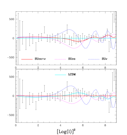
Figure 1: Left panel: Transfer functions (multiplied by $k^{1.5}$, for graphic aims) in example cosmologies with/without coupling and with/without 2 massive $\nu$’s (00/CM models). Right panel: Binned anisotropy spectral data, normalized to the best–fit $\Lambda$CDM model (upper frame) or to the best fit SUGRA cDE model including $\nu$–masses (lower frame). The distorsions arising when coupling or $\nu$–mass are separately considered are also shown.

The simplest coupling is a linear one, formally obtainable through a conformal transformation of Brans–Dicke theory (see, e.g., brans ). The coupling intensity must however be adequate to transfer from CDM to DE the energy needed to beat its spontaneous dilution $\propto a^{-6}$. This prescribes a coupling scale $C^{-1}\sim m_{p}$, while the energy drain from CDM lets its density decline (slightly) more rapidly than $a^{-3}$. The whole scenario between recombination and the birth of non linearities is then modified, and it comes as no surprise that we expect significant changes both in the matter density fluctuation spectra $P(k)$ and in the observed angular anisotropy spectrum $C_{l}$.

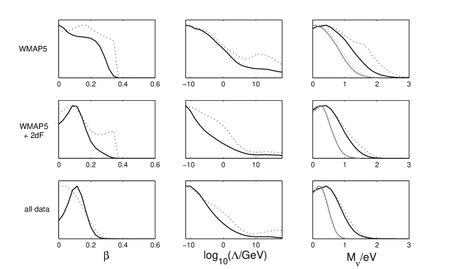
Figure 2: Marginalized (solid line) and average (dotted line) likelihood of cosmological parameters in SUGRA models. Notice that the $\beta$ signal appears when high– and low–$z$ data are put together, and is strengthened by SNIa data. As a matter of fact, coupling allows to lower the “tension” between $\Omega_{c}$ and fluctuation amplitude detected from CMB and deep sample data. For $M_{\nu}$ we also show the corresponding likelihood distributions obtained in the case of a standard $\Lambda$CDM+$M_{\nu}$ model (gray lines).

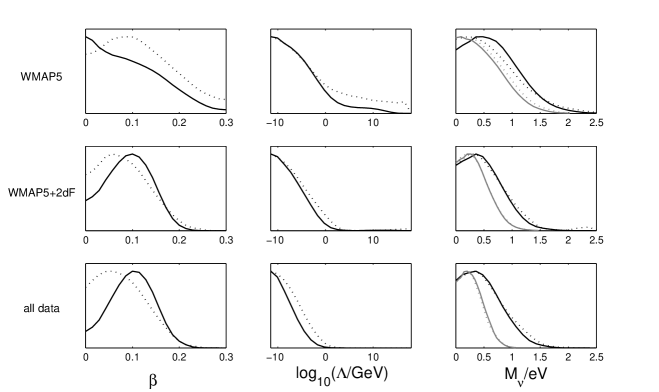
Figure 3: As previous Figure, in RP models.

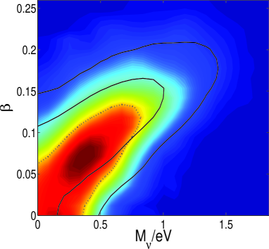
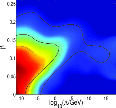
Figure 4: Two parameter contours for the SUGRA model. Solid lines are 1– and 2–$\sigma$ limits for marginalized likelihood. Colors refer to average likelihood, and the 50% likelihood contour from the average likelihood is indicated by the dotted line.

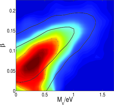
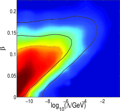
Figure 5: As previous Figure, for a RP potential.

The prescription that the 2–component dark sector interacts with baryons or radiation only through gravitaion reads $T^{(c)~{}\mu}_{~{}~{}~{}~{}\nu;\mu}+T^{(de)~{}\mu}_{~{}~{}~{}\,~{}~{}\nu;\mu}=0$  (here $T^{(c,de)}_{\mu\nu}$ are the stress–energy tensors for CDM and DE, let their traces read $T^{(c,de)}$). Only if we make the further assumption that the 2 components are separate, it shall be $C\equiv 0$ in the relations

$$T^{(de)~{}\mu}_{~{}~{}~{}\,~{}~{}\nu;\mu}=+CT^{(c)}\phi_{,\nu}~{},~{}~{}T^{(c)~{}\mu}_{~{}~{}~{}~{}\nu;\mu}=-CT^{(c)}\phi_{,\nu}~{},$$ (7)

obtained by passing from the Jordan frame, where a Brans–Dicke frame cosmology holds, to the Einstein frame coupling ; brans . These equations also show why DE cannot couple to any component with vanishing stress–energy tensor trace, e.g. to radiation.

Besides of $C$, we shall also use the dimensionless coupling parameter $\beta=(3/16\pi)^{1/2}m_{p}C~{}.$ If it is $C=1/m_{p}$, therefore, $\beta=0.2443$; values $\beta\sim$$\cal O$$(0.1)$ mean then $C\simeq 1/2m_{p}~{}$.

In this context let us then remind the interesting option of considering DE coupled to $\nu$’s mavans ; the trace $T^{(\nu)}$ becomes significant only when their kinetic energy is redshifted to values $\sim m_{\nu}$.

Another option considered in the literature is that the r.h.s.’s of eqs. (7) are replaced by $\pm\bar{C}T^{(de)}\phi_{,\nu}$, where $\bar{C}$ sign is opposite to $C$ spagnoletti . This option causes a bootstrap effect, as the energy transfer to DE is boosted as soon as its dilution is attenuated. In analogy with the coupling to $\nu$’s, this approach therefore associates the peculiarity of our epoch (the coincidence) with another accepted peculiarity. Furthermore, at variance from our approach, this option does not follow from any conformal transformation of Brans–Dicke formulation.

It should be however noticed that the correlation between $M_{\nu}$ (the trace of the 3-dimensional neutrino mass matrix) and $C$ seems no longer to persist within the frame of this approach if new datasets are considered spagnoletti2 .

2 Procedure and Results

The results shown in this paper are based on our generalization of the public program CAMB camb , enabling it to study cDE models. Likelihood distributions are then worked out by using CosmoMC lewis:2002 .

In Figure 1 we then illustrate the compensating effects between coupling and $\nu$ mass, by considering various cosmologies. A 00–model is then a cosmology without coupling and $\nu$ mass. In turn, the 01– and 10–models are cosmologies with coupling (and no $\nu$ mass) and $\nu$ mass (and 0–coupling). In the 11–model, finally, both $\nu$ mass and coupling are included.

The l.h.s. plot shows an example of transfer functions for 00–, 01–, 10– and 11–models. The sum of $\nu$ masses ($M_{\nu}$) is tuned so that the 00– and 11– $T(k)$’s nearly coincide. At the r.h.s., we then see a similar comparison with $C_{l}$ anisotropy spectral data. More details are provided in the caption.

More details on the fitting procedure are provided elsewhere kristiansen09 . The fitting procedure returns parameter values mostly in the same range as for dDE or $\Lambda$CDM cosmologies. The significant parameters in our approach are however the energy scale in potentials ($\Lambda$), the coupling intensity ($\beta$), and the sum of $\nu$ masses ($M_{\nu}$). In Figures 2 and 3 we provide one–dimensional likelihood distributions on these parameters for SUGRA and RP cosmologies.

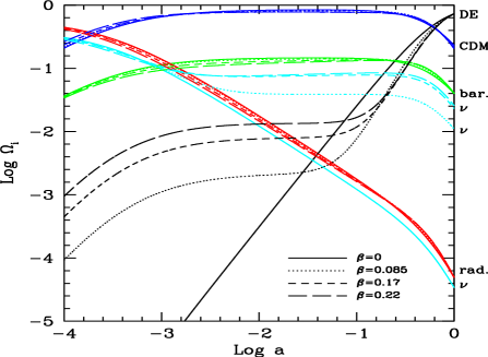
Figure 6: Evolution of density parameters in a SUGRA model with coupling and $\nu$ mass. Colors refer to different components, as specified in the frame; lines to the different models: $M_{\nu}=0,~{}\beta=0$ (continuous line); $M_{\nu}=0.5~{}$eV, $\beta=0.085$ (dotted); $M_{\nu}=1.1~{}$eV, $\beta=0.17$ (short dashed); $M_{\nu}=1.2~{}$eV, $\beta=0.22$ (long dashed).

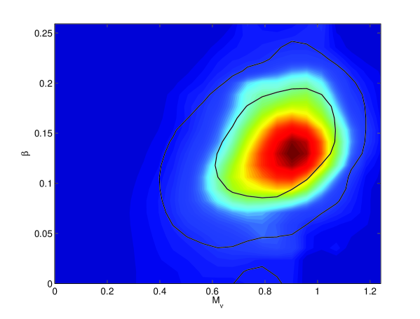
Figure 7: Detection of CDM–DE coupling, following an hypothetical determination of an electron neutrino mass $m_{\nu}\simeq 0.3~{}$eV, by the experiment KATRIN, yielding $M_{\nu}\simeq 0.9~{}$eV. Here we show the likelihood distribution, with such a prior on $M_{\nu}$. Colors and lines convey the same indications as in Figures 4 and 5.

A basic information is however the correlation between likelihood distributions. These are shown in Figures 4 and 5 again for SUGRA and RP cosmologies, respectively.

These Figures, as well as one–dimensional plots, clearly exhibit maxima, both for average and marginalized likelihood, for significantly non–zero coupling and $\nu$–masses. Although their statististical significance is not enough to indicate any “detection” level, the indication is impressive. Furthermore, a stronger signal, with the present observational sensitivity, would be impossible.

Let us however outline that this work aimed at finding how far one could go from $\Lambda$CDM, adding non–zero coupling and $\nu$–mass, without facing a likelihood degrade. It came then as an unexpected bonus that likelihood does not peak on the 0–0 option.

3 Conclusions

The allowed $\beta$ values open the possibility of a critically modified DE behavior. Figure 6 shows the scale dependence of the cosmic components for various $\beta$–$M_{\nu}$ pairs.

For $\beta$ values comprised between 0.1 and 0.22, i.e. well within 2–$\sigma$’s from the best–fit model, just as the 0–0 option, we have a long plateau in the energy density of DE, going from $z\sim 10$ to above $z=1000$. The devline of $\rho_{de}$ at greater $z$ is then mostly due to a parallel decline of the density $\rho_{c}$ of CDM: when radiation becomes dominant, both DCM and DE are negligible.

The ratio $\rho_{c}/\rho_{de}$ in the plateau is $\cal O$$(100)$. At lower $z$ it becomes gradually smaller because of the gradual contribution of the potential term to $\rho_{de}$. It should be however outlined that this behavior is not ad–hoc, but is incribed in the tracker solutions for the potentials selected.

Let us finally outline that the $M_{\nu}$ values allowed by $\beta\sim 0.1$–0.2 approach the $\nu$–mass detection area in the forthcoming experiment KATRIN katrin , based on tritium decay.

Accordingly, should particle data lead to an external prior on $M_{\nu}$, the strong degeneracy between the coupling parameter $\beta$ and the neutrino mass $M_{\nu}$ is broken, and new insight into the nature of DE is gained kristiansen09 . In Figure 7 we show how a neutrino mass determination symultaneously implies an almost model independent CDM–DE coupling detection.

This would be a revival of mixed DM models mix , in the form of Mildly Mixed Coupled (MMC) cosmologies.

References

- (1) Phillips M.M. et al. A.J. 104, 1543 (1992); A. G. Riess, R. P. Kirshner, B. P. Schmidt, S. Jha, et al., Astrophys. J. 116, 1009 (1998); S. Perlmutter, G. Aldering, G. Goldhaber, et al., Astrophys. J. 517, 565 (1999); then see also, e.g.. A. G. Riess, L.G. Strolger, J. Tonry, et al., Astrophys. J. 607, 665 (2004), A.C. Becker et al., arXiv:0811.4424 (astro-ph, 2008).
- (2) P. de Bernardis et al., Nat. 404, 955 (2000); S. Padin et al., Astrophys. J. 549, L1 (2001); J. Kovac, E. Leitch, C. Pryke, et al., Nat. 420, 772 (2002); D. Spergel, R. Bean, Dorè et al., Astrophys. J. Suppl. 170, 377 (2007), E. Komatsu et al. [WMAP Collaboration], arXiv:0803.0547 [astro-ph].
- (3) M. Colless, G. Dalton, S. Maddox, et al., Mon. Not. R. Astron. Soc. 329, 1039 (2001); M. Colless, B. Peterson, C. Jackson, et al., Preprint astro–ph/0306581; J. Loveday (the SDSS collaboration), C.P. 43, 437 (2002); M. Tegmark, M. Blanton, M. Strauss, et al., Astrophys. J. 606, 702 (2004); J. Adelman–McCarthy, M. Agueros, S. Allam, et al., Astrophys. J. Suppl. 162, 38 (2004).
- (4) L. Colombo & M. Gervasi, JCAP 10, 001 (2006).
- (5) Wetterich C., A&A 301, 321 (1995); Amendola L., Phys. Rev. D62, 043511 (2000).
- (6) G. La Vacca, S. A. Bonometto and L. P. L. Colombo, New Astron. 14, 435 (2009)
- (7) Ratra B. & Peebles P.J.E. (1988) PR D37, 3406.
- (8) Brax P and Martin J 1999 Phys. Lett. B468 40; Brax P and Martin J 2000 Phys. Rev. D61 103502
- (9) Damour T., Gibbons G. W. & Gundlach C., 1990, Phys.Rev., L64, 123D Damour T. & Gundlach C., 1991, Phys.Rev., D43, 3873
- (10) L. Amendola, Phys. Rev. D 60, 043501 (1999); V. Pettorino and C. Baccigalupi, Phys. Rev. D 77, 103003 (2008)
- (11) P. Gu, X. Wang and X. Zhang, Phys. Rev. D68, 087301 (2003); R. Fardon, A. E. Nelson & N. Weiner, JCAP 0410 005 (2004); N. Afshordi, M. Zaldarriaga & K. Kohri, Phys. Rev. D 72, 065024 (2005); O. E. Bjaelde et al., JCAP 0801, 026 (2008); V. Pettorino and C. Baccigalupi, Phys. Rev. D 77, 103003 (2008); Franca U., Lattanzi M., Lesgourgues J. & Pastor S., Phys. Rev. D 80, 083506 (2009)
- (12) M. B. Gavela, D. Hernandez, L. Lopez Honorez, O. Mena, and S. Rigolin, ArXiv e-prints (Jan., 2009) [0901.1611].
- (13) B. A. Reid, L. Verde, R. Jimenez and O. Mena, arXiv:0910.0008 [astro-ph.CO].
- (14) A. Lewis, A. Challinor & A. Lasenby, Astrophys. J. , 538, 473 (2000); http://www.camb.info/.
- (15) A. Lewis and S. Bridle 2002 Phys. Rev. D 66, 103511
- (16) KATRIN collaboration. KATRIN design report 2004. http://wwwik. fzk.de/ katrin/publications/documents/DesignReport2004-12Jan2005.pdf, 2005.
- (17) J.R. Kristiansen, G. La Vacca, L.P.L. Colombo, R. Mainini, S. A. Bonometto, arXiv:0902.2737 [astro-ph] (2009); G. La Vacca, J.R. Kristiansen, L.P.L. Colombo, R. Mainini, S. A. Bonometto, JCAP 0904, 007 (2009)
- (18) S.A. Bonometto & R. Valdarnini, Phys. Lett. A 104, 369 (1984); R. Valdarnini & S. Bonometto, A&A 146, 235 (1985); R. Valdarnini & S. Bonometto, Astrophys. J. 299, L71 (1985); Achilli S., Occhionero F. & Scaramella R., Astrophys. J. 299, 577 (1985)