Abstract

We study photonic, neutrino and charged particle signatures from slow decays of gravitino dark matter in supersymmetric theories where R-parity is explicitly broken by trilinear operators. Photons and (anti-)fermions from loop and tree-level processes give rise to spectra with distinct features, which, if observed, can give crucial input on the possible mass of the gravitino and the magnitude and flavour structure of R-violating operators. Within this framework, we make detailed comparisons of the theoretical predictions to the recent experimental data from PAMELA, ATIC and Fermi LAT.

1 Introduction

In recent years, there has been a revived interest in the possibility of gravitino dark matter within the framework of R-violating supersymmetry [1, 2]. There are several reasons for this. In the much-studied CMSSM [3], scenarios with neutralino dark matter have become rather constrained, requiring a considerable amount of fine-tuning. The additional fact that R-parity is imposed essentially by hand, and alternative schemes are equally viable from the theoretical point of view, has motivated the search for other dark matter candidates. In the case that R-parity is violated, neutralinos and other sparticles decay too fast to be dark matter, even for small couplings, however, this is not the case for gravitinos, which raise very interesting possibilities. Indeed, if gravitinos decay slowly enough for their lifetime to exceed the age of the universe [4, 5], they can be considered essentially stable and a good dark matter candidate. While cosmologically stable, gravitinos may still have decays of interest to astrophysics measurements of cosmic rays in various particle species.

Trilinear R-violating couplings have the form

$$\lambda L_{i}L_{j}{\bar{E}}_{k}+\lambda^{\prime}L_{i}Q_{j}{\bar{D}_{k}}+\lambda^{\prime\prime}{\bar{U}_{i}}{\bar{D}_{j}}{\bar{D}_{k}},$$ (1.1)

where $L(Q)$ are the left-handed lepton (quark) doublet superfields, and ${\bar{E}}$ (${\bar{D}},{\bar{U}}$) are the corresponding left-handed singlet fields. Due to SU(2) and SU(3) invariance, we have 9 $L_{i}L_{j}{\bar{E}_{k}}$ operators $(i\neq j)$, 27 $L_{i}Q_{j}{\bar{D}_{k}}$, and 9 ${\bar{U}_{i}}{\bar{D}_{j}}{\bar{D}_{k}}$ operators $(j\neq k)$. These couplings are known to give rise to very interesting collider phenomenology, with the missing energy signature of the much studied Minimal Supersymmetric Standard Model (MSSM) being in part substituted by multi-lepton and/or multi-jet events [6].

The same R-violating operators that lead to the decay of sparticles produced in collider experiments, will also cause gravitino dark matter to decay. This takes place via two-body radiative loop decays to neutrino and photon [2], and via tree-level decays to three fermions [5]. The decay rates have been presented in detail in the original references, where it was found that, for light gravitino masses and appropriate fermions in the loop, radiative decays may dominate, while for heavier gravitinos, three-body decays take over. The behavior of the total decay rate is primarily controlled by the gravitino mass dependence of the partial decay widths. These scale as

$$\Gamma_{\tilde{G}} \propto m_{\tilde{G}}^{7}\quad\text{(three-body decays),}$$ (1.2)

$$\Gamma_{\tilde{G}} \propto m_{\tilde{G}}\quad\text{(radiative decays),}$$ (1.3)

for three-body decays away from the kinematic threshold, and radiative decays with gravitino masses well below those of the next-to-lightest supersymmetric particle (NLSP) and sufficiently above the kinematic threshold of its decay products. Moreover, the results are very dependent on the flavour structure of R-violating operators, which is discussed extensively in [7].

To constitute a realistic dark matter candidate, the minimal requirement is that the gravitino lifetime should exceed the age of the universe, which may naturally occur due to the Planck scale suppression in the gravitino vertex, the smallness of the R-parity-violating coupling, and the additional loop/phase-space suppression in the radiative/tree-level diagrams. In addition, cosmic rays from slow gravitino decays have to be consistent with observations, e.g. the photon flux measured in the EGRET experiment [8]. The extra-galactic photon flux has been shown to set severe bounds on gravitino decays and thus on the allowed combinations of gravitino masses and R-violating couplings [1, 2, 7, 9]. Recently, new results on the flux of charged particles have been published by the ATIC [10], PAMELA [11, 12], and Fermi LAT Collaborations [13]. These show possible excesses that, modulo unknown astrophysical sources, could signal New Physics.

One could also consider the possibility of tree level decays to a neutrino and photon through neutrino–neutralino mixing. This decay width is directly proportional to the R-parity violating operators’ contribution to the neutrino masses. For a given choice of basis [6], this in turn depends on the alignment between the vevs of the neutral scalar components of the superfields $(H_{d},L_{i})$ and the coefficients of the bilinear terms $(\mu,\mu_{i})$, where $\mu_{i}H_{u}L_{i}$ are potentially non-zero bilinear R-violating operators.

The expected charged particle spectra of mixing induced decays have recently been studied in detail in [14, 15, 16, 17], and the neutrino spectra in [18]. The alignment angle is very restricted in order to comply with neutrino mass bounds, and a completely general phenomenological model allows these decays to be sub-dominant to the decays discussed above. Thus, our present Letter complements these analyses for the case of decays dominated by trilinear R-violating operators. As we will demonstrate, under certain assumptions on the background electron spectrum, it is possible to simultaneously fit the PAMELA data on the positron and antiproton fractions and the Fermi LAT data on the electron-plus-positron spectrum. Such a fit requires high gravitino masses, and the resulting gamma ray spectrum predicted from electron bremsstrahlung should be testable with the upcoming Fermi LAT data. For the neutrinos we find that their flux will be very difficult to detect in both present and near-future experiments.

This Letter is structured as follows: In Section 2, we study charged fermion and anti-fermion spectra from gravitino decays using a standard galactic propagation model. We attempt a fit to the PAMELA and Fermi LAT data, discussing the limitations of the background model, and we set limits on the R-parity violating couplings as a function of the gravitino mass. In Section 3, after discussing our procedure and the handling of experimental uncertainties, we proceed to a study of photonic spectra; we discuss the information that can be obtained from characteristic peaks directly linked to the magnitude and flavour of the R-violating couplings, the mass of the gravitino and the SUSY spectrum. Furthermore, we make predictions corresponding to our best fits to the PAMELA and Fermi LAT data, and show that these can be tested in the near future, either supporting our considerations, or setting even more severe bounds on R-violating couplings. In Section 4 we discuss the potential for observation of the neutrino spectra from gravitino decays. Finally in Section 5 we summarise our results and look at future prospects.

2 Charged particles

Gravitinos decaying through the tree level diagrams that are induced by trilinear R-violating operators, will produce charged particles, which, for appropriate values of the gravitino mass and the R-violating couplings may help to explain recent experimental data on cosmic rays. Of particular interest in this respect is the measurement of the cosmic ray positron fraction by PAMELA [11] and the Fermi LAT results [13] on the cosmic ray electron spectrum that both show excesses, but in somewhat different energy ranges. In addition, the non-observation of any anomaly in the antiproton data as reported by PAMELA[12] is important in constraining the possible parameter space.

2.1 Model

We calculate the electron, positron and antiproton spectra in the gravitino rest frame for a particular gravitino mass and R-violating coupling. We study the decay of gravitinos using PYTHIA 6.4 [20], and the branching ratios and lifetime given by the formulae in [5, 7]. After being produced, charged particles will propagate through the galaxy. Although we have substantial information about the various processes that give important contributions, this propagation still contains large uncertainties. For a recent review of cosmic ray propagation, see [21].

The most important propagation effects come from diffusion processes caused by galactic magnetic fields and scattering off magnetohydrodynamic (MHD) waves; this spatial diffusion causes the received spectra to be essentially isotropic. The scattering off MHD waves also causes diffusion in momentum space known as diffusive re-acceleration. It is also possible that an important role is played by convection due to galactic winds. At present, it seems that the most appropriate model for galactic propagation is a diffusion model, possibly extended with some convection [21]. On top of this, charged particles are losing energy due to synchrotron radiation, bremsstrahlung, ionization and inverse Compton scattering.

To take all these effects into account, we use the GALPROP code [22] with a conventional diffusion model, similar to ‘model 0’ in [23]. The main parameters adopted for GALPROP are given in Table 1. The dark matter component of the various fluxes incident on the earth has been calculated assuming a Navarro-Frenk-White (NFW) [24] dark matter density profile for our galaxy:

$$\rho_{\text{Halo}}(r)=\frac{\rho_{0}}{(r/r_{c})(1+r/r_{c})^{2}},$$ (2.1)

where $r$ denotes the distance to the center of the galaxy, $r_{c}=20$ kpc and $\rho_{0}=0.33$ GeV cm^-3.

$D_{0}~{}[\text{cm}^{2}\text{ s}^{-1}]$	$\delta$	$z_{h}~{}[\text{kpc}]$	$\gamma_{0}$	$N_{e^{-}}~{}[\text{cm}^{-2}\text{ s}^{-1}\text{ sr}^{-1}\text{ GeV}^{-1}]$	$\gamma_{0}^{P}$
$5.75\times 10^{28}$	0.34	4	2.50	$4.0\times 10^{-7}$	2.36

Table 1: GALPROP parameters. With the diffusion coefficient $D$ assumed to have a power-law dependence on the energy, with index $\delta$, $D_{0}$ denotes its value at $4$ GeV; $z_{h}$ is the half-height of the halo in which the cosmic rays are assumed to propagate. Finally, $\gamma_{0}$ and $N_{e^{-}}$ give the spectral index and normalization (at $34.5$ GeV) of the electron injection spectrum, while $\gamma_{0}^{P}$ is the spectral index of the nuclei injection spectra.

At low energy, below 5–10 GeV, the resulting background spectra for both positrons and antiprotons in this model deviate somewhat from the data. This is believed to be due to solar modulation effects [11], and not any potential New Physics. For the positron fraction, therefore, only points above 10 GeV are used for our fits.

2.2 Positrons and electrons

Cosmic ray electrons and positrons are usually divided into primary cosmic rays originating in cosmic accelerators such as e.g. supernova remnants (SNR), and secondary cosmic rays stemming from cosmic rays (mostly protons) interacting with the interstellar medium [25]. Positrons are, unlike electrons, believed to originate mostly from secondary cosmic rays [21]. At the energies of interest, the secondary cosmic ray particle spectrum can be assumed to be charge symmetric, with the secondary positrons and electrons having the same spectrum. The primary electrons, together with secondary electrons and positrons, are expected to give an exponentially falling electron-plus-positron spectrum, as well as positron fraction, at high energy [23].

Recently, several deviations from this picture have been observed in cosmic ray electron and positron data. The PAMELA Collaboration [11] has observed a steep rise in the positron fraction above 10 GeV, with the data continuing up to 100 GeV. In addition, ATIC [10] and Fermi LAT [13] have both reported anomalous structures in the electron-plus-positron spectra up to around 800 GeV. These anomalies seem to indicate a hitherto unknown source of primary electrons and positrons. This has lead to a lot of theoretical activity trying to explain both spectral features within various dark matter models, while at the same time avoiding severe constraints from current gamma-ray data, due to radiation from the annihilation or decay products of the dark matter candidate.

In what follows, we will investigate how well the features of the PAMELA and Fermi LAT data can be explained by decaying gravitinos. Since there is some discrepancy between ATIC and Fermi LAT, in particular at energies above 300 GeV, we focus on the Fermi LAT data, due to the smaller errors. The ATIC data, having a less smooth spectrum, cannot be fitted as well as the Fermi LAT data in the present scenario. In general, one can say that the ATIC data prefers a slightly harder spectrum than Fermi LAT, thus operators with more pronounced electron flavour (see below) would be favored.

The main source of high-energy electrons and positrons in gravitino decays with trilinear R-violating operators is the direct production of charged leptons as occurs for $LL\bar{E}$ and $LQ\bar{D}$ operators. For a given gravitino mass and electron-flavour lepton number violating operator we get a hard spectrum of direct electrons and positrons, while for second and third generation lepton number violating operators and the same gravitino mass we get softer spectra from the decays of $\mu$ and $\tau$. In the case of hadronic tau decays, as well as the direct production of quarks, we get many lower-energy electrons from the decay of charged pions.

To fit the PAMELA data with $LL\bar{E}$ operators is rather straightforward; it is in fact possible to get a decent fit with any such operator, provided the gravitino mass is sufficiently large (most require a gravitino mass of at least 320 GeV). Also $LQ\bar{D}$ operators can be used given a $L_{1}$ operator and a suitable gravitino mass. In Fig. 1 we show three examples where $L_{1}L_{2}\bar{E}_{1}$, $L_{1}L_{3}\bar{E}_{3}$ and $L_{1}Q_{2}\bar{D}_{2}$ have been used to fit the PAMELA data by varying the coupling for a $m_{\tilde{G}}=320~{}\text{GeV}$ gravitino, while assuming a common mass of $m_{\rm SUSY}=1$ TeV for the other sparticles. The details of the fits are given in Table 2.

Figure 1: Data on positron fraction from PAMELA (red, with error bars) compared to GALPROP background (solid blue) and fitted contributions from $m_{\tilde{G}}=320~{}\text{GeV}$ gravitino decaying through an $L_{1}L_{2}\bar{E}_{1}$ operator (dashed blue), an $L_{1}L_{3}\bar{E}_{3}$ operator (green) and an $L_{1}Q_{2}\bar{D}_{2}$ operator (red). The left panel shows the standard GALPROP background, in the right panel the primary electron spectrum has been rescaled by a factor 0.75.

	GALPROP background			Rescaled background
Coupling	$\lambda$	$\tau~{}[10^{26}\text{ s}]$	$\chi^{2}_{\text{PAM}}/{\rm ndf}$	$\lambda$	$\tau~{}[10^{26}\text{ s}]$	$\chi^{2}_{\text{PAM}}/{\rm ndf}$
$\lambda_{121}$	$6.2\times 10^{-8}$	3.9	2.7	$4.1\times 10^{-8}$	8.9	0.3
$\lambda_{133}$	$8.1\times 10^{-8}$	2.3	0.3	$5.5\times 10^{-8}$	5.0	1.4
$\lambda^{\prime}_{122}$	$9.3\times 10^{-8}$	1.7	0.6	$6.2\times 10^{-8}$	3.8	2.1

Table 2: Best fit values for R-violating couplings to the PAMELA positron fraction for $m_{\tilde{G}}=320$ GeV and $m_{\text{SUSY}}=1$ TeV. The respective gravitino lifetimes and the fit quality are also shown.

The background spectra of primary electrons from SNRs, as well as the secondary electrons and positrons, have been calculated by GALPROP. Which operator gives the best fit to data is sensitive to the assumptions entering into the calculation. If the standard GALPROP parameters given above are used, as shown in Fig. 1 (left panel), operators with less direct production of positrons and thus flatter spectra, $L_{1}L_{3}\bar{E}_{3}$ and $L_{1}Q_{2}\bar{D}_{2}$, give a better fit. On the other hand, a small rescaling of the primary electrons by a factor 0.75 favors the steeper rise given by the $L_{1}L_{2}\bar{E}_{1}$ operator (right panel).

Given this sensitivity to small changes in the background assumptions for the PAMELA positron fraction, we will not discuss in further detail which operators are more favored by PAMELA alone. Nor will we go to the other extreme and attempt a global fit of all data, as this would require a sophisticated treatment of experimental errors and the propagation model that go beyond the scope of this Letter. Instead, we adopt a simple approach where we investigate whether it is possible to fit the Fermi LAT data, and at the same time retain a reasonable fit quality to the PAMELA data, allowing for small adjustments in the background assumptions. In order to simultaneously explain both data sets, we find that it is sufficient to scale down the background of primary electrons somewhat compared to the conventional GALPROP model. In what follows, we have adopted a simple rescaling factor of 0.75.

Let us begin with some generic lessons learned concerning operator flavours and gravitino masses, when attempting to fit both data-sets. In order to fit the Fermi LAT data alone, a minimal requirement is a rather high gravitino mass, of at least $m_{\tilde{G}}\gtrsim 1.5$ TeV. However, for most operators, even higher gravitino masses are required. Given such a large gravitino mass, it is important not to have a too steep spectrum in order to simultaneously explain the PAMELA rise, which takes place at a much lower energy than the Fermi LAT excess. This can be best achieved with a significant amount of tau flavour in the operator. We find that operators of the type $L_{i}L_{j}\bar{E}_{3}$ are most suitable for a simultaneous fit, since they require at least one tau in the final state of the gravitino decay. At the same time, operators of the type $L_{i}L_{j}\bar{E}_{1}$ seem excluded as an explanation of both anomalies, due to their too steep spectra: the magnitude of the coupling that is required in order to explain PAMELA gives too large a contribution to the electron spectra at higher energies. Finally, to have a sufficiently large contribution to the high energy electron spectra, one either needs some electron flavour in the operator, $i=1$ or $j=1$, or an even higher gravitino mass.

The qualitative description above is quantified in Table 3, which lists the operators we find capable of simultaneously fitting both the Fermi LAT and the PAMELA data, i.e. in statistical terminology operators with $\chi^{2}$ such that we fail to reject them at the 5% significance level. Table 3 also gives the $1\sigma$ error on the gravitino mass; both the gravitino mass and the error are given from a two-parameter ($\lambda$ and $m_{\tilde{G}}$) maximum likelihood fit to the Fermi LAT data.

Under the assumption of a single coupling dominance, the value of the coupling $\lambda$ does not affect the shape of the particle spectrum, but only its normalization. As a result, the statistical error on the coupling for a given gravitino mass is quite small, around 2–3%, far smaller than the possible systematic errors on the data normalization from the energy scale in the experiments [13]. Therefore we only give the value of the coupling for the best fit gravitino mass. The behaviour of the coupling as a function of the gravitino mass around the best fit, $\lambda\propto m_{\tilde{G}}^{-3.5}$, is clear from the gravitino width dependence in the three-body decay, Eq. (1.2). We also give the gravitino lifetime for the best fit gravitino mass and the $\chi^{2}$ of the fit decomposed into the individual contributions from the two data sets, divided by the degrees of freedom: for PAMELA $n=7$, and for Fermi LAT $n-1=25$. Note that for the coupling $\lambda^{\prime}_{133}$ we have not conducted any fit of the gravitino mass. This is because it cannot simultaneously fit both the Fermi LAT and the PAMELA data. It is included in Table 3 merely for future reference.

Coupling	$m_{\tilde{G}}\ [\text{TeV}]$	$\lambda$ at best fit	$\tau\ [10^{26}\text{ s}]$	$\chi^{2}_{\text{PAM}}$	$\chi^{2}_{\text{Fermi}}$
$\lambda_{123}$	1.8${}^{+0.1}_{-0.2}$	$7.3\times 10^{-9}$	2.0	1.0	0.9
$\lambda_{132}$	1.8${}^{+0.1}_{-0.1}$	$6.9\times 10^{-9}$	2.3	1.7	1.1
$\lambda_{133}$	1.8${}^{+0.1}_{-0.3}$	$8.0\times 10^{-9}$	1.7	0.6	0.8
$\lambda_{232}$	2.8${}^{+0.4}_{-0.2}$	$1.7\times 10^{-9}$	1.5	1.6	1.1
$\lambda_{233}$	3.6${}^{+0.6}_{-0.3}$	$8.7\times 10^{-10}$	0.9	0.4	0.6
$\lambda^{\prime}_{133}$	1.8	$7.8\times 10^{-10}$	1.3	27	0.8

Table 3: Operators for which the Fermi LAT and PAMELA electron and positron data can be fitted simultaneously. $\lambda$ and $\tau$ are given for the central gravitino mass value for a given operator (see text). All other sparticle masses entering the calculation are set to 6 TeV. In the case of $\lambda^{\prime}_{133}$ the mass has not been fitted and the sparticle masses used here are 2 TeV (hence the smaller coupling).

As seen in Table 3, the best fits are given by $L_{1}L_{3}\bar{E}_{3}$ with a $1.8$ TeV gravitino and $L_{2}L_{3}\bar{E}_{3}$ with a $3.6$ TeV gravitino. These two fits are shown in Fig. 2, where we also include a comparison to HESS data on the electron spectrum at even higher energies [27]. It is, however, important to keep in mind that, even if an operator cannot fit the data by itself, it might still do so in combination with some other suitable operator.

Figure 2: Left panel: fit of $L_{1}L_{3}\bar{E}_{3}$ operator with $m_{\tilde{G}}=1.8$ TeV and $m_{\text{SUSY}}=6$ TeV (dashed blue), $L_{2}L_{3}\bar{E}_{3}$ operator with $m_{\tilde{G}}=3.6$ TeV and $m_{\text{SUSY}}=6$ TeV (dotted blue) and GALPROP background (solid blue) to electron-plus-positron spectrum from Fermi LAT (red, with error bars). Also shown is ATIC data (green, with error bars) and HESS data (violet inverted triangles, with error bars). Right panel: data on positron fraction from PAMELA (red, with error bars) shown with GALPROP background (solid blue) and the result of the fit for the $L_{1}L_{3}\bar{E}_{3}$ (dashed blue) and $L_{2}L_{3}\bar{E}_{3}$ (dotted blue) operators.

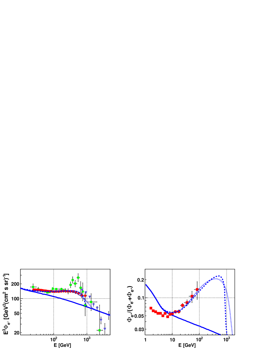
If we were to consider the excess seen in the HESS spectrum at around 1 TeV [27] in the fits, there would be some preference for the higher ends of the gravitino mass regions; for $L_{1}L_{3}\bar{E}_{3}$ and $L_{1}L_{2}\bar{E}_{3}$ one would need $m_{\tilde{G}}>2$ TeV, while $L_{2}L_{3}\bar{E}_{3}$, due to its softer cut-off at high energy, fits the HESS data more naturally.

So far we have exclusively fitted to the Fermi LAT data and ignored the ATIC data. It is of course possible to fit to the ATIC data instead. As has been mentioned above, this favors a larger amount of electron flavour in the operator and it turns out that the best operator for the ATIC data is $L_{2}L_{3}\bar{E}_{1}$. Since the ATIC data is less smooth than the Fermi LAT data, it is not possible to fit it equally well. The large error bars in the peak of the ATIC data also reduce the tension between the electron-plus-positron data and the positron fraction data, suggesting that fitting to Fermi LAT is the more reasonable and constraining approach.

It is also possible to achieve a reasonable fit to the Fermi LAT data with $LQ\bar{D}$ operators that contain $L_{1}$. The best such example is $L_{1}Q_{3}\bar{D}_{3}$, which is shown in Fig. 3; however, $LQ\bar{D}$ operators cannot fit simultaneously the PAMELA and Fermi LAT data, due to positron excesses at low energies. We shall see below that the interpretation in terms of $LQ\bar{D}$ operators is also clearly excluded by the PAMELA antiproton data.

Figure 3: Similar to Fig. 2 for an $L_{1}Q_{3}\bar{D}_{3}$ operator with $m_{\tilde{G}}=1.8$ TeV and $m_{\text{SUSY}}=2$ TeV.

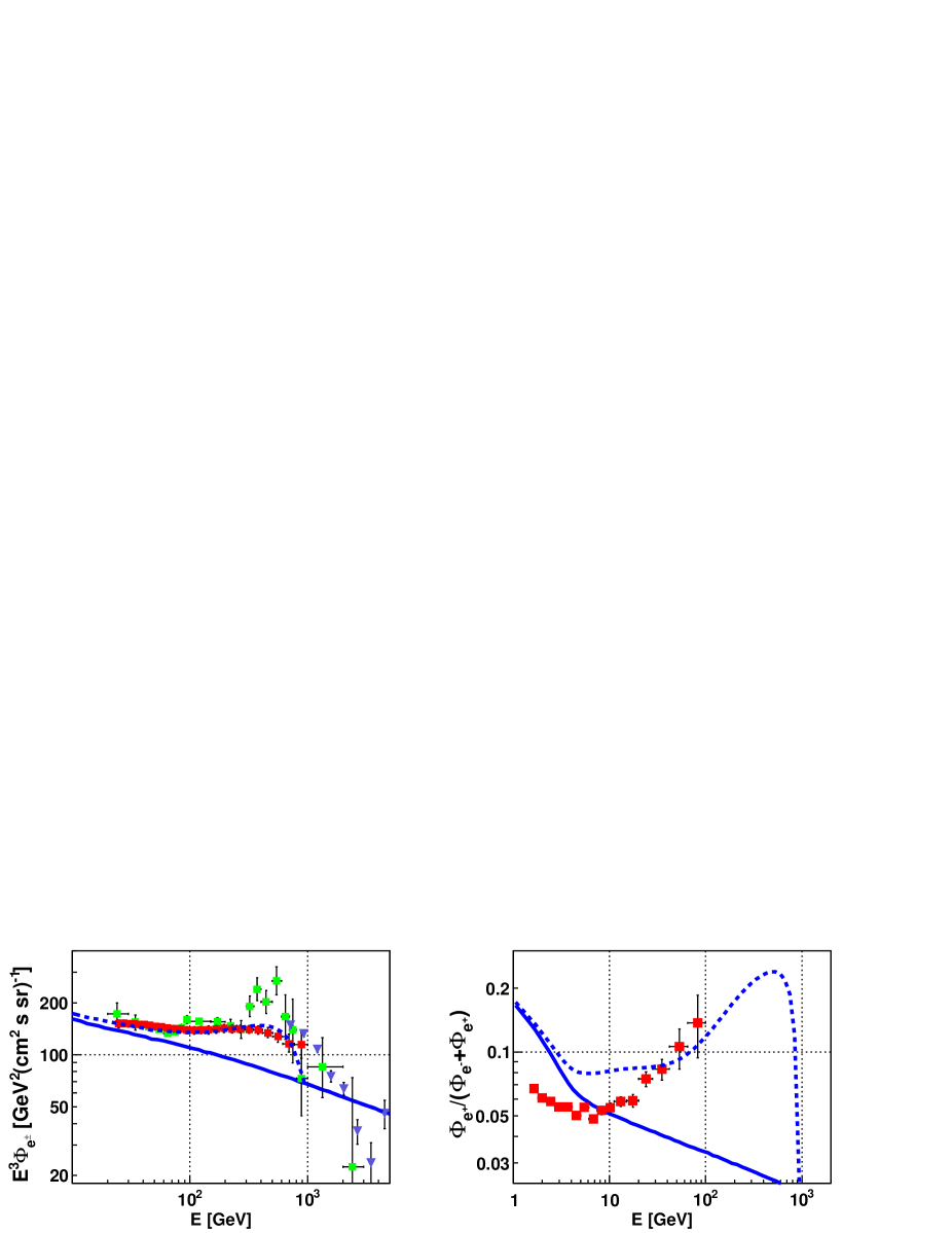
It is interesting to note some important differences between this scheme and dark matter annihilation scenarios: direct annihilation to lepton pairs gives a large contribution of monochromatic electrons and positrons in the CM frame. Even when galactic propagation is taken into account, it is difficult to achieve the smooth excess over the background spectrum that is observed by Fermi LAT. Consequently, dark matter annihilation to an electron-positron pair seems largely excluded as an explanation of the Fermi LAT [28] excess. For gravitino decays, on the other hand, the three-body phase space can naturally give rise to the smooth shape observed.

Let us finally comment on the consequences of the above for the LHC. As can be seen in Table 3, due to the large gravitino masses and the $m_{\tilde{G}}^{7}$ dependence of the gravitino decay width, the R-parity violating couplings need to be very small in order to fit the data, $\mathcal{O}(10^{-9})$. This implies that, in such a scheme, R-parity violation cannot be observed at the LHC unless the NLSP is charged and can be stopped. The large sparticle masses required also imply that the production cross section is very low, if at all non-zero.

2.3 Antiprotons

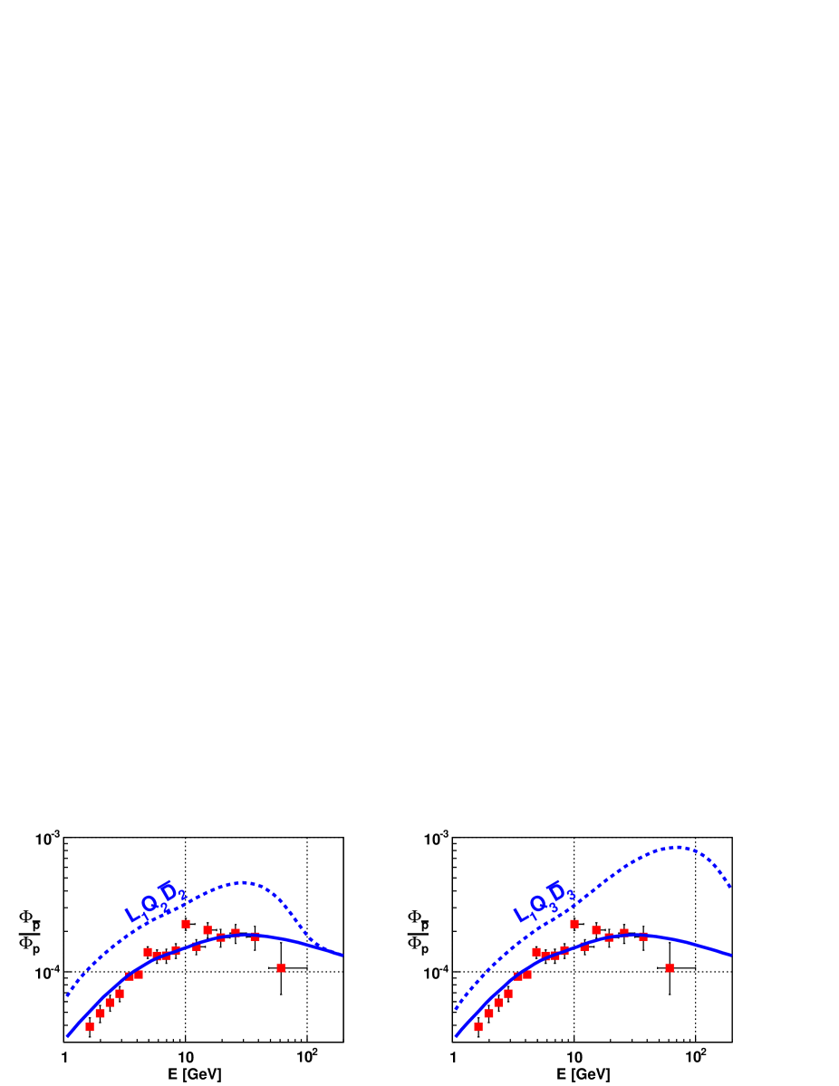
In the case of $LQ\bar{D}$ and $\bar{U}\bar{D}\bar{D}$ operators, one would also expect production of protons and antiprotons within the quark jets. The PAMELA antiproton data [12] give rather tight constraints on all $LQ\bar{D}$ and $\bar{U}\bar{D}\bar{D}$ couplings for high gravitino masses. In Fig. 4 we show the antiproton fraction data and compare to fits to the PAMELA positron fraction (left) and the Fermi LAT electron-plus-positron flux data (right). In both cases the $LQ\bar{D}$ operators that fit the lepton data overproduce antiprotons, and are effectively ruled out. From Fig. 4 we can also see that the pure background is fairly consistent with the data, considering the potential for large systematic errors. $LL\bar{E}$ operators on the other hand, do not produce any antiprotons and are therefore not affected by these bounds.

Figure 4: PAMELA data on the antiproton fraction (red, with error bars) compared to the GALPROP background (solid blue) and the contribution from the best fit to the PAMELA positron fraction using the $L_{1}Q_{2}\bar{D}_{2}$ operator (left, dashed blue) and the best fit to the Fermi LAT electron-plus-positron spectrum with the $L_{1}Q_{3}\bar{D}_{3}$ operator (right, dashed blue). The parameters of the fits can be found in Tables 2 (“rescaled background”) and 3, respectively.

2.4 Maximal couplings

From the above discussion, it follows that the R-violating couplings can be significantly constrained by the charged particle data. We determine such limits by varying the gravitino mass and the coupling, while restricting the operator to give a total flux that does not exceed any data point by more than $3\sigma$.

To be conservative when setting the bounds there are no backgrounds included in these calculations, except in the case of the positron fraction where the electron background has to be included in order to get a meaningful result; the positron background, however, is not included. In contrast to the fits, we are using here the full spectra of the PAMELA data. Given the relatively small experimental uncertainties at lower energies, and having excluded the background from the calculation, we should still get robust constraints, despite the solar modulation uncertainties at the lowest energies.

We present the resulting bounds for a representative selection of operators in Fig. 5. For comparison we also show the limits on the coupling from the EGRET gamma-ray data for $L_{1}L_{2}\bar{E}_{1}$. For details on the derivation of this limit and comparisons between gamma-ray constraints on different operators, see [7]. In Fig. 5 we use $m_{SUSY}=1$ TeV, for other sparticle masses one can use the scaling $\lambda_{max}\propto m_{SUSY}^{2}$. The range in gravitino mass shown is chosen to be comparable with earlier work [7], and to cover the range where RPV decays at the LHC might be possible.

Figure 5: Maximum allowed couplings $\lambda_{\max}$ versus gravitino mass, derived from the Fermi LAT electron-plus-positron data (solid), the PAMELA positron fraction data (dot-dashed) and antiproton data (dashed). We show bounds for the $L_{1}L_{2}\bar{E}_{1}$ (red), $L_{2}L_{3}\bar{E}_{3}$ (blue), $L_{1}Q_{2}\bar{D}_{2}$ (green) and $\bar{U}_{1}\bar{D}_{1}\bar{D}_{2}$ (violet) operators. For comparison, the constraint derived from the EGRET gamma ray data in [7] is shown for $L_{1}L_{2}\bar{E}_{1}$ (solid black).

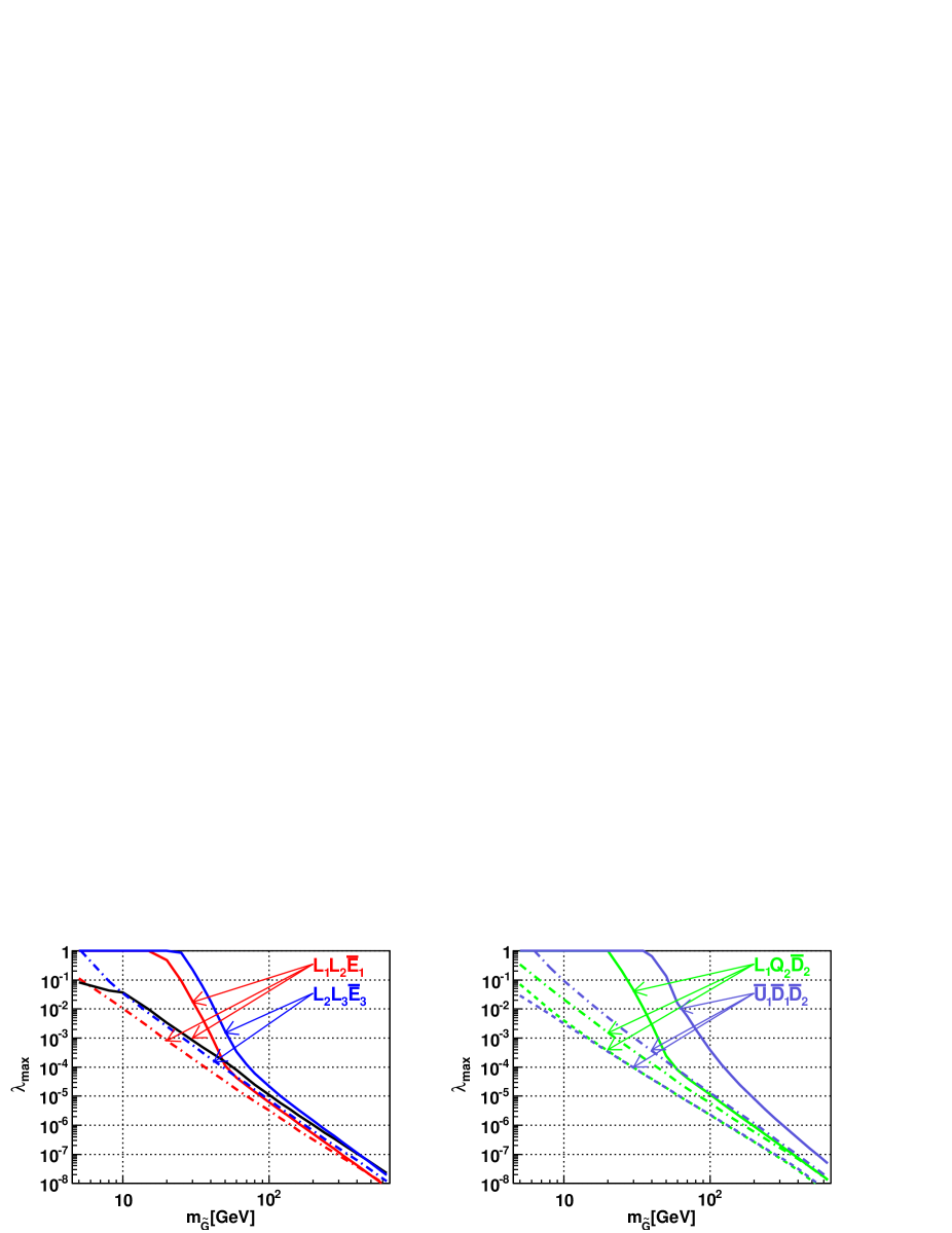
For $LL\bar{E}$ operators, the positron fraction data gives the most constraining bounds for medium to high gravitino masses. As expected, this bound is stronger for operators with direct positron production, e.g. $L_{1}L_{2}\bar{E}_{1}$, as compared to indirect production, via $L_{2}L_{3}\bar{E}_{3}$. At low gravitino masses, the operators that allow radiative loop decays, such as $L_{1}L_{2}\bar{E}_{1}$, will be mainly constrained by the gamma-ray data, while at very high masses the constraints from the electron-plus-positron data is competitive. For $LQ\bar{D}$ operators we observe a similar behaviour, however, in this case the antiproton data provide even stronger bounds. Finally, $\bar{U}\bar{D}\bar{D}$ operators have no radiative decays and no direct electron/positron production, but produce both positrons and gammas from pion decays, resulting in bounds similar to, but weaker than, the bounds on the $LQ\bar{D}$ operators. As expected the antiproton data is more restrictive; the constraint from antiprotons turns out to be almost identical to the one for $LQ\bar{D}$ operators. This is something of a numerical accident, $\bar{U}\bar{D}\bar{D}$ operators give more antiprotons, but the $LQ\bar{D}$ operators have roughly twice the gravitino decay width for the same coupling strength, and these effects cancel each other out.

Overall, we see that for gravitino masses smaller than the values required to fit PAMELA and Fermi LAT, the allowed couplings can be significantly larger and will result in observable R-violation at the LHC.

3 Photon Spectra

In this section we discuss the photon spectra from gravitino decays, and the possibility of either excluding or strengthening the gravitino interpretation of the electron and positron excesses using current and future gamma-ray measurements.

The data we use for comparison is the extragalactic spectrum from EGRET as calculated by [29]. The choice of this data over the first EGRET analysis [8] is due to the improved background modeling in [29].

3.1 Model

There are three main contributions to the gamma-ray spectrum from gravitino decays: there is direct photon production in the radiative loop decays (giving a monochromatic component), there are photons from internal bremsstrahlung of charged particles, and there are photons from pion decays. In this case as well, we let PYTHIA [20] simulate the gravitino decay including all relevant decay channels. The photon spectrum reaching the earth can be further divided into two components; one extragalactic part that has been red-shifted from its energy in the gravitino rest frame and one part from the galactic halo.

The extragalactic contribution to the total flux is given by [9]

$$\left[E^{2}\frac{dJ}{dE}\right]_{\text{EG}}=\frac{2E^{2}}{m_{\tilde{G}}}C_{\gamma}\int^{\infty}_{1}dy\frac{dN_{\gamma}}{d(Ey)}\frac{y^{-3/2}}{\sqrt{1+\kappa y^{-3}}},$$ (3.1)

where $y=1+z$, $z$ being the redshift, and $dN_{\gamma}/dE$ the gamma ray spectrum from the gravitino decay in its rest frame, as calculated by PYTHIA. The constants $C_{\gamma}$ and $\kappa$ are given by

$$C_{\gamma}=\frac{\Omega_{\tilde{G}}\rho_{c}}{8\pi\tau_{\tilde{G}}H_{0}\Omega_{M}^{1/2}}\quad{\rm and}\quad\kappa=\frac{\Omega_{\Lambda}}{\Omega_{M}}.$$ (3.2)

The halo component has been calculated using the NFW [24] dark matter halo profile of Eq. (2.1), which has been averaged over all directions such that $|b|\geq 10^{\circ}$, where $b$ denotes galactic latitude. This exclusion is done in order to avoid the difficult background of strong gamma ray sources within the galactic disc, and mimics what is done in the analysis of the EGRET data [29] that we will be comparing to. The halo component of the flux is then given as

$$\left[E^{2}\frac{dJ}{dE}\right]_{\text{Halo}}=\frac{E^{2}}{m_{\tilde{G}}}\frac{dN_{\gamma}}{dE}\frac{1}{4\pi\tau_{\tilde{G}}}\int_{\text{los}}\rho_{\text{Halo}}{\vec{l}}d\vec{l},$$ (3.3)

where $\int_{los}\rho_{Halo}{\vec{l}}d\vec{l}$ is the line-of-sight integral averaged over the specified part of the halo profile. The resulting gamma ray spectra have also been smoothed to account for the effects of a detector with energy resolution of 15%, again on the basis of the properties of the EGRET analysis.

In Fig. 6 we show photon spectra for different flavour combinations in the R-violating couplings, demonstrating the variety of possible gamma-ray spectral shapes that can be generated. To illustrate the potential observable consequences of decaying gravitino dark matter in a gamma-ray experiment, we pick the R-parity violating couplings in such a way that the spectrum is close to the EGRET measurement, and for comparison we also show the EGRET data [29].

Figure 6: Photon spectra for four representative R-violating operators: $L_{1}L_{2}\bar{E}_{1}$ (top left), $L_{1}L_{2}\bar{E}_{3}$ (top right), $L_{1}Q_{3}\bar{D}_{3}$ (bottom left) and $\bar{U}_{2}\bar{D}_{1}\bar{D}_{2}$ (bottom right), for the following set of parameters: $m_{\tilde{G}}=40$ GeV, $M_{\text{SUSY}}=200$ GeV, and $\lambda=10^{-5}$. We show the extragalactic (red) and halo (green) contributions, as well as the total (blue). Also shown is the EGRET data.

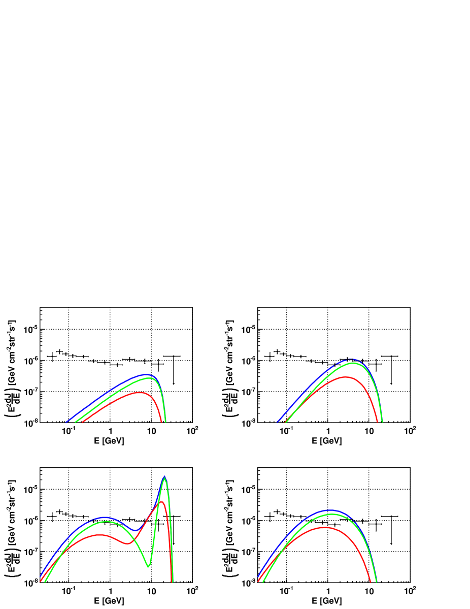
From Fig. 6 we observe that the two-body decays (when present, such as in the lower left plot) tend to dominate and the result is a monochromatic line at $m_{\tilde{G}}/2$. In an experiment this would then show up as a broad peak; however, a gravitino mass could potentially be identified if sufficient statistics were available, the accuracy limited mostly by the experimental resolution. Furthermore, we observe the following:

• When all decay products are electrons and muons (top-left panel) practically all gamma radiation comes from internal bremsstrahlung. This radiation is quite hard and has a sharp cut-off at $m_{\tilde{G}}/2$.

• For $LL\bar{E}$ operators with some $\tau$ flavour (top-right panel) gamma rays come from both internal bremsstrahlung and decaying mesons from tau decays, mostly $\pi^{0}$, giving a softer spectrum as compared to only bremsstrahlung, for the same gravitino mass.

• In the case of $L_{i}Q_{3}\bar{D}_{3}$ operators (bottom-left panel) we get a combination of photons from loop and tree-level decays (the latter give photons through decaying mesons). The heavier the particle in the loop, the larger the loop contribution; $L_{i}Q_{3}\bar{D}_{3}$ has the most pronounced loop contribution of all operators, due to the high mass of the b-quark [2].

• Finally, for $\bar{U}\bar{D}\bar{D}$ couplings (bottom-right panel), the only sizable contribution arises through meson decays, resulting in a soft spectrum.

3.2 Predictions from PAMELA and Fermi LAT

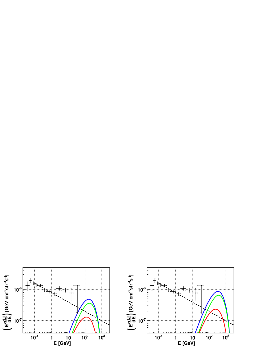
We can now make predictions for what should be observed in gamma-ray experiments assuming that the PAMELA and Fermi LAT data discussed in the previous section are explained by trilinear R-parity violating operators. As we have seen, the only option is to use $LL\bar{E}$ operators and large gravitino masses, above 1 TeV. In this range, three-body decays are likely to completely dominate, implying the absence of an observable peak of monochromatic photons. However, with such high gravitino masses, a considerable photon flux is still expected from bremsstrahlung and pion decays.

In Fig. 7 we show the predictions from two of the fits in Section 2 ($L_{1}L_{3}\bar{E}_{3}$ and $L_{2}L_{3}\bar{E}_{3}$) compared to the EGRET data. It is clear that both predictions are compatible with the data because the large gravitino mass implies that the dark matter spectrum lies outside the EGRET sensitivity range. However, new Fermi LAT data on gamma rays is expected to cover at least parts of this region, and our best fit models predict a broad spectral feature whose position is correlated to the gravitino mass. Assuming a power-law like continuation of the EGRET data this feature may be observed, or our present models excluded. If both the rise and the cut-off of the feature is observed, an estimate of a probable gravitino mass may be made, and the type and size of the R-violating coupling could be further constrained.

Figure 7: Photon spectra for the best-fit models of Fig. 2; $\lambda_{133}=8.0\times 10^{-9}$, $m_{\tilde{G}}=1.8$ TeV (left) and $\lambda_{233}=8.7\times 10^{-10}$, $m_{\tilde{G}}=3.6$ TeV (right). We show the extragalactic (red) and halo (green) contributions, as well as the total (blue). For comparison we also give the EGRET data, and a power-law continuation of the data in the interval [0.05,2] GeV (dashed line).

4 Neutrinos

In addition to the photon flux, the two-body decay mode also generates a monochromatic neutrino flux in the gravitino rest frame. Moreover, in the three-body decays, neutrinos will be produced both in the initial decay, and in subsequent decays of unstable leptons and hadrons. Neutrinos, like photons, travel essentially undeflected from the point of production. However, they undergo oscillations, changing from one flavour to another over distances which are small compared to galactic scales.

Ignoring possible CP violation in the neutrino sector, the transition probabilities can be expressed in terms of the mixing matrix $U$ as

$$P(\nu_{\alpha}\to\nu_{\beta})=\sum_{k=1}^{3}(U_{\alpha k}U_{\beta k})^{2}.$$ (4.1)

For the mixing we adopt the parameters of [30], corresponding to maximal mixing between the $\mu$ and $\tau$ flavours, $\sin^{2}\theta_{23}=0.5$, and for the remaining mixings $\sin^{2}\theta_{12}=0.304$ and $\sin^{2}\theta_{13}=0.01$. This gives:

$$\begin{split}&P(\nu_{e}\leftrightarrow\nu_{e})=0.56\,,\\ &P(\nu_{e}\leftrightarrow\nu_{\mu})=P(\nu_{e}\leftrightarrow\nu_{\tau})=0.22\,,\\ &P(\nu_{\mu}\leftrightarrow\nu_{\mu})=P(\nu_{\mu}\leftrightarrow\nu_{\tau})=P(\nu_{\tau}\leftrightarrow\nu_{\tau})=0.39\,.\end{split}$$ (4.2)

The effect of the above is to erase flavour specific information from the decay in the neutrinos that reach us. However, it also guarantees the presence of muon neutrinos in the flux, which, for the near future, seems to be our best hope for detection through the production of muons in the scattering off nucleons in experiments such as IceCube. For electron neutrinos, the resulting electron energy in the present model is too low for reconstruction of the neutrino direction, making a rejection of the enormous background from cosmic ray showers difficult, while tau neutrinos contribute to the muon flux with a fraction corresponding to the tau branching ratio into muons.

Due to the similarities in the propagation, the neutrino flux is calculated in analogy with the gamma ray flux, i.e., by the use of Eqs. (3.1) and (3.3), taking into account neutrino oscillations. The resulting neutrino spectra have then been smoothed to mimic a 10% energy resolution on muons in a detector. This smoothening causes the energy spectra to exceed the theoretical upper limit of $m_{\tilde{G}}/2$. In this simple model we have ignored the energy lost to the accompanying hadronic shower, the inelasticity of the event, which should further smear the spectrum toward lower energies. We also restrict ourselves to through-going muons, and ignore the muon energy loss in matter. For a more thorough treatment of these effects for generic models of decaying dark matter, see [33].

The resulting muon neutrino spectrum is shown in Fig. 8 (left) for the best-fit models shown in Fig. 2. We compare this signal to the expected atmospheric neutrino background spectrum taken from [34]. Figure 8 (right) also shows the expected number of signal and background events per year in the IceCube experiment, calculated by folding the neutrino spectra with the effective area of a completed IceCube experiment averaged over the northern hemisphere [35].

Figure 8: Neutrino $(\nu_{\mu}+\bar{\nu}_{\mu})$ spectrum (left) and expected number of events in IceCube (right) for best fit models (blue) discussed in Section 2 (dashed: $\lambda_{133}=8.0\times 10^{-9}$, $m_{\tilde{G}}=1.8$ TeV, dotted: $\lambda_{233}=8.7\times 10^{-10}$, $m_{\tilde{G}}=3.6$ TeV), compared to atmospheric neutrino flux (black, solid) .

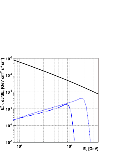
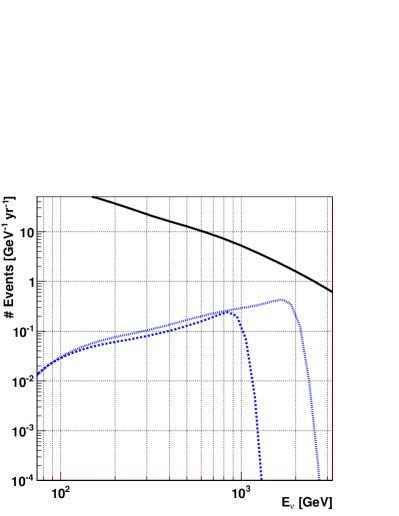
It is worth noting that the similarity at low neutrino energies and the difference in cut-off between the two models shown in Fig. 8 is a direct consequence of the fit to the Fermi LAT electron-plus-positron data and its limited reach in energy shown in Fig. 2. The model with larger gravitino mass fits the HESS data beyond Fermi LAT better. Thus, observing a cut-off in the Fermi LAT excess will predict the position of the cut-off in the neutrino spectrum in these models and vice versa.

We can see from Fig. 8 (left) that neutrinos directly produced from the three-body $LL\bar{E}$ decays give an enticing peak in the neutrino flux around $m_{\tilde{G}}/2$. However, large atmospheric backgrounds make the detection of these neutrinos very challenging. For IceCube we expect ${\mathcal{O}}(500)$ upward going muons per year in total from these neutrinos for the best case scenario with the largest gravitino mass. This seems marginal when compared to an expected total atmospheric background of 25k events per year. When using the spectral feature of the flux, the numbers are more encouraging, we find $S/\sqrt{B}=5.4$ and $S/B=0.19$ for events in the energy interval $1.6-2.0$ TeV.

One possible route to improvements is to look instead at downward going muons where efficient rejection of muon neutrinos produced in cosmic ray events may become feasible with the IceCube DeepCore detector [36, 37]. This was recently discussed for leptophilic dark matter in [38].

5 Summary-outlook

In this work, we have studied the expected charged particle, photon and neutrino spectra of slowly decaying gravitino dark matter within the framework of supersymmetric models with explicitly broken R-parity through trilinear operators. We identify couplings that generate spectra with a distinct behaviour that may reproduce recent experimental photon and (anti-)fermion data. Among others, we find the following:

• The cosmic ray electron and positron data, as reported by the PAMELA Collaboration, can be easily reproduced via $LL\bar{E}$ and $LQ\bar{D}$ operators. Couplings with significant electron flavour give rise to a hard spectrum, in contrast to the case where most electrons come from $\mu$ and $\tau$ decays. In the case of tau as well as quark final states, low energy electrons are produced from the decay of charged pions. We find that most operators require a gravitino mass of at least 320 GeV to explain the PAMELA data.

• In order to fit the Fermi LAT data alone, we need even higher gravitino masses, of at least $m_{\tilde{G}}\gtrsim 1.5$ TeV (for most operators significantly larger). In order to simultaneously account for the PAMELA rise, which takes place at a much lower energy, such gravitino masses also require a part of the spectrum that is not too hard, favoring operators of the $L_{i}L_{j}\bar{E}_{3}$ type. Sufficiently large contributions to the high energy electron spectrum can then be obtained either via some electron flavour in the operator ($i=1$ or $j=1$) or by going to even higher gravitino masses. The decaying dark matter scenario discussed in this Letter has a significant advantage over dark matter annihilation scenarios, where it is hard to achieve a spectrum that is smooth enough to explain the electron excess observed by Fermi LAT.

• $L_{1}Q_{j}\bar{D}_{k}$ operators may give a reasonable fit to the Fermi LAT data alone, but cannot then fit the PAMELA data due to positron excesses at low energies and the over-production of antiprotons. In fact, the PAMELA antiproton data give very tight constraints on all $LQ\bar{D}$ and $\bar{U}\bar{D}\bar{D}$ couplings for high gravitino masses.

• For the range of gravitino masses that can match the PAMELA and Fermi LAT data, three-body decays are likely to dominate, implying the absence of the observable peak of monochromatic photons found in two-body radiative gravitino decays. Large photon fluxes are still expected, due to bremsstrahlung off charged particles and pion decays. Such fluxes are a necessary consequence of our scenario and should be detectable by Fermi LAT for parameters that can explain the charged particle excesses, meaning that Fermi LAT will be capable of supporting or ruling out this explanation of the electron and positron anomalies.

• Neutrinos directly produced from the three-body decays have a quite sharp peak around $m_{\tilde{G}}/2$, which, with the sharp rise in effective area with energy, gives some hope of future detection at IceCube. In particular, despite only measuring the muon energy from the neutrino interaction, this may lead to a better gravitino mass determination than what is possible from bremsstrahlung photons.

Summarising, it is interesting to observe that our predictions on the basis of the PAMELA and Fermi LAT data are very restrictive, and imply that in the future this scenario will either be confirmed, or very strict bounds will be imposed on R-violating couplings for heavy gravitino masses. It is also interesting to note that R-violating couplings too small to detect at the LHC, can be probed through the study of photon and (anti-)particle spectra.

Acknowledgements. The work of NEB and PO has been supported by the Research Council of Norway. SL has been funded by the FP6 Marie Curie Excellence Grant MEXT-CT-2004-014297 and also acknowledges support by the European Research and Training Network UniverseNet, MRTPN-CT-2006 035863-1. ARR is grateful for financial support from the Swedish Research Council (VR) through the Oskar Klein Centre and thanks Chad Finley for enlightening discussions.

References

- [1] W. Buchmuller, L. Covi, K. Hamaguchi, A. Ibarra and T. Yanagida, JHEP 0703 (2007) 037 [arXiv:hep-ph/0702184].
- [2] S. Lola, P. Osland and A. R. Raklev, Phys. Lett. B 656 (2007) 83 [arXiv:0707.2510 [hep-ph]].
- [3] A. H. Chamseddine, R. Arnowitt and P. Nath, Phys. Rev. Lett. 49 (1982) 970; L. E. Ibanez, Phys. Lett. B 118 (1982) 73; K. Inoue, A. Kakuto, H. Komatsu and S. Takeshita, Prog. Theor. Phys. 68 (1982) 927 [Erratum-ibid. 70 (1983) 330]; Prog. Theor. Phys. 71 (1984) 413; J. R. Ellis, D. V. Nanopoulos and K. Tamvakis, Phys. Lett. B 121 (1983) 123; L. Alvarez-Gaume, J. Polchinski and M. B. Wise, Nucl. Phys. B 221 (1983) 495.
- [4] F. Takayama and M. Yamaguchi, Phys. Lett. B 485 (2000) 388 [arXiv:hep-ph/0005214].
- [5] G. Moreau and M. Chemtob, Phys. Rev. D 65 (2002) 024033 [arXiv:hep-ph/0107286].
- [6] R. Barbier et al., Phys. Rept. 420 (2005) 1 [arXiv:hep-ph/0406039].
- [7] N.-E. Bomark, S. Lola, P. Osland and A. R. Raklev, Phys. Lett. B 677 (2009) 62 arXiv:0811.2969 [hep-ph].
- [8] P. Sreekumar et al. [EGRET Collaboration], Astrophys. J. 494 (1998) 523 [arXiv:astro-ph/9709257].
- [9] A. Ibarra and D. Tran, Phys. Rev. Lett. 100 (2008) 061301 [arXiv:0709.4593 [astro-ph]].
- [10] J. Chang et al., Nature 456 (2008) 362.
- [11] O. Adriani et al. [PAMELA Collaboration], Nature 458 (2009) 607 [arXiv:0810.4995 [astro-ph]].
- [12] O. Adriani et al., Phys. Rev. Lett. 102 (2009) 051101 [arXiv:0810.4994 [astro-ph]].
- [13] A. A. Abdo et al. [The Fermi LAT Collaboration], Phys. Rev. Lett. 102, 181101 (2009) [arXiv:0905.0025 [astro-ph.HE]].
- [14] A. Ibarra and D. Tran, JCAP 0807, 002 (2008) [arXiv:0804.4596 [astro-ph]]; JCAP 0902, 021 (2009) [arXiv:0811.1555 [hep-ph]].
- [15] W. Buchmuller, A. Ibarra, T. Shindou, F. Takayama and D. Tran, JCAP 0909, 021 (2009) [arXiv:0906.1187 [hep-ph]].
- [16] K. Ishiwata, S. Matsumoto and T. Moroi, Phys. Rev. D 78, 063505 (2008) [arXiv:0805.1133 [hep-ph]].
- [17] K. Ishiwata, S. Matsumoto and T. Moroi, Phys. Lett. B 675, 446 (2009) [arXiv:0811.0250 [hep-ph]].
- [18] L. Covi, M. Grefe, A. Ibarra and D. Tran, JCAP 0901, 029 (2009) [arXiv:0809.5030 [hep-ph]].
- [19] S. L. Chen, R. N. Mohapatra, S. Nussinov and Y. Zhang, Phys. Lett. B 677, 311 (2009) [arXiv:0903.2562 [hep-ph]].
- [20] T. Sjostrand, S. Mrenna and P. Skands, JHEP 0605 (2006) 026 [arXiv:hep-ph/0603175].
- [21] A. W. Strong, I. V. Moskalenko and V. S. Ptuskin, Ann. Rev. Nucl. Part. Sci. 57 (2007) 285 [arXiv:astro-ph/0701517].
- [22] A. W. Strong and I. V. Moskalenko, Adv. Space Res. 27 (2001) 717 [arXiv:astro-ph/0101068].
- [23] D. Grasso et al. [FERMI-LAT Collaboration], Astropart. Phys. 32, 140 (2009) [arXiv:0905.0636 [astro-ph.HE]].
- [24] J. F. Navarro, C. S. Frenk and S. D. M. White, Astrophys. J. 490 (1997) 493 [arXiv:astro-ph/9611107].
- [25] I. V. Moskalenko, A. W. Strong and S. G. Mashnik, AIP Conf. Proc. 769 (2005) 1612 [arXiv:astro-ph/0411400].
- [26] V. Barger, Y. Gao, W. Y. Keung, D. Marfatia and G. Shaughnessy, Phys. Lett. B 678 (2009) 283 [arXiv:0904.2001 [hep-ph]].
- [27] F. Aharonian et al. [H.E.S.S. Collaboration], Phys. Rev. Lett. 101 (2008) 261104 [arXiv:0811.3894 [astro-ph]].
- [28] P. Meade, M. Papucci, A. Strumia and T. Volansky, arXiv:0905.0480 [hep-ph].
- [29] A. W. Strong, I. V. Moskalenko and O. Reimer, Astrophys. J. 613 (2004) 956 [arXiv:astro-ph/0405441]; Astrophys. J. 613 (2004) 962 [arXiv:astro-ph/0406254].
- [30] A. Strumia and F. Vissani, arXiv:hep-ph/0606054.
- [31] H. Yuksel, S. Horiuchi, J. F. Beacom and S. Ando, Phys. Rev. D 76, 123506 (2007) [arXiv:0707.0196 [astro-ph]].
- [32] S. Palomares-Ruiz, Phys. Lett. B 665, 50 (2008) [arXiv:0712.1937 [astro-ph]].
- [33] L. Covi, M. Grefe, A. Ibarra and D. Tran, arXiv:0912.3521 [hep-ph].
- [34] M. Honda, T. Kajita, K. Kasahara, S. Midorikawa and T. Sanuki, Phys. Rev. D 75 (2007) 043006 [arXiv:astro-ph/0611418].
- [35] T. Montaruli, Nucl. Phys. Proc. Suppl. 190 (2009) 101 [arXiv:0901.2661 [astro-ph]].
- [36] S. Schonert, T. K. Gaisser, E. Resconi and O. Schulz, Phys. Rev. D 79 (2009) 043009 [arXiv:0812.4308 [astro-ph]].
- [37] C. Wiebusch for the IceCube Collaboration, arXiv:0907.2263 [astro-ph.IM].
- [38] S. K. Mandal, M. R. Buckley, K. Freese, D. Spolyar and H. Murayama, arXiv:0911.5188 [hep-ph].