Abstract

It has been shown recently that phantom-like effect can be realized on the normal branch of the DGP setup without introduction of any phantom matter neither in the bulk nor on the brane and therefore without violation of the null energy condition. It has been shown also that inclusion of the Gauss-Bonnet term in the bulk action modifies this picture via curvature effects. Here, based on the Lue-Starkman conjecture on the dynamical screening of the brane cosmological constant in the DGP setup, we extend this proposal to a general DGP-inspired $f(R,\phi)$ model that stringy effects in the ultra-violet sector of the theory are taken into account by inclusion of the Gauss-Bonnet term in the bulk action. We study cosmological dynamics of this setup, especially its phantom-like behavior and possible crossing of the phantom divide line especially with a non-minimally coupled quintessence field on the brane. In this setup, scalar field and curvature quintessence are treated in a unified framework.
PACS: 98.80.-k, 95.36.+x, 98.80.Cq
Key Words: Braneworld Cosmology, Dark Energy, Scalar-Tensor Theories, Modified Gravity

1 introduction

Recent evidences from supernova searches data [1,2], cosmic microwave background (CMB) results [3-5] and also Wilkinson Microwave Anisotropy Probe (WMAP) data [6,7,8], show an positively accelerating phase of the cosmic expansion today and this feature shows that the simple picture of the universe consisting of the pressureless fluid is not enough to describe the cosmological dynamics. In this regard, the universe may contain some sort of the additional negative-pressure dark energy. Analysis of the WMAP data [9-11] shows that there is no indication for any significant deviations from Gaussianity and adiabaticity of the CMB power spectrum and therefore suggests that the universe is spatially flat to within the limits of observational accuracy. Further, the combined analysis of the WMAP data with the supernova Legacy survey (SNLS) [9], constrains the equation of state $\omega_{de}$, corresponding to almost $74\%$ contribution of dark energy in the currently accelerating universe, to be very close to that of the cosmological constant value. In this respect, a $\Lambda$CDM ( Cosmological constant plus Cold Dark Matter) model has maximum agreement with the recent data, but with an unnaturally small and fine-tuned value of $\Lambda$ [4]. From the general relativity viewpoint, such models simply modify the right hand side of the Einstein’s field equations by including in the stress-energy tensor something more than the usual matter and radiation components. As a radically different approach, one can also try to leave the source side unchanged, but rather modifying the geometric sector in the left-hand side. In this viewpoint, the cosmic speed up can be interpreted as a first signal of the breakdown of the laws of physics as encoded by the standard General Relativity. This is essentially reasonable: the General Relativity has been experimentally tested only up to the Solar System scale and there is no a priori theoretical motivation to extend its validity to extraordinarily larger scales such as the cosmological ones. Extending General Relativity without giving up its positive results, opens the way to a large class of alternative theories of gravity ranging from extra-dimensions [12] to non-minimally coupled scalar fields [13,14,15]. In particular, fourth order theories [16,17,18] based on replacing the scalar curvature $R$ in the Einstein-Hilbert action with a generic analytic function $f(R)$ have attracted a lot of attention in the last decade. Also referred to as $f(R)$ gravity, these models have been shown to be able to both fit the cosmological data and evade the Solar System constraints in several physically interesting cases [19-28]. In this sense, modified gravity provides the very natural gravitational alternative for dark energy. Also modified gravity presents very natural unification of the early-time inflation and late-time acceleration due to different role of gravitational terms relevant at small and at large curvature [29,30,31]. Moreover, some models of modified gravity are predicted by string/M-theory considerations [16,17,18].

In the framework of braneworld scenarios, a possible approach to realize the late-time acceleration of the universe is to consider modification of gravity on the appropriate scales. This can be achieved for instance by a weakening of gravitational interaction at large scales. Weakening of gravity on large scales provides an effective negative pressure that drives the late-time acceleration of the universe. The Dvali, Gabadadze and Porrati (DGP) scenario [32] is one of the simplest scenario in this regard. In this model, our universe is a brane embedded in a Minkowski 5D bulk space-time. Standard matter and gauge interactions are trapped on the brane and only gravity experiences the full bulk. Cosmological dynamics in this setup follows two distinct branches of solutions: self-accelerating and the normal branch [33,34,35]. Late-time acceleration can be explained in the self-accelerating branch without invoking any unknown dark energy component. However, the normal branch requires a dark energy component to accommodate the current observations [36-45]. Although the self-accelerating branch explains the late-time acceleration in a fascinating manner, it suffers from serious theoretical problems such as the ghost issue [46]. Fortunately the normal branch is free from instabilities. Recently it has been shown that the normal branch of the DGP braneworld scenario which is not self-accelerating can realize phantom-like behavior without introducing any phantom field on the brane [36-45]. By phantom-like behavior we mean an effective energy density which is positive and grows with time and its equation of state parameter stays always less than $-1$. Other extensions to realize this phantom-like behavior are studied in Refs. [47-66]. On the other hand, dark energy models with non-minimally coupled scalar field and other extensions of scalar-tensor theories have been studied widely some of which can be found in references [67-71].

In the spirit of scalar-tensor dark energy models, our motivation here is to show that a general $f(R,\phi)$ GBIG-inspired scenario can account for late-time acceleration and crossing of the phantom divide line in some suitable domains of model parameters space. To show this feature, first we study cosmological dynamics of $f(R,\phi)$ GBIG-inspired scenario briefly. In the minimal case, motivated by modified theories of gravity, some authors have included a term of the type $l_{0}R^{n}$ in the action [72-77]. This extension for some values of $n$ has the capability to explain late-time acceleration of the universe in a simple manner. It is then natural to extend this scenario to more general embeddings of DGP inspired scenarios.

The purpose of this paper is to perform such a generalization to study both late-time acceleration and possible crossing of the phantom divide line in this setup. we construct a braneworld scenario with modified induced gravity on the brane and the Gauss-Bonnet term in the bulk action. We study cosmological dynamics of this setup and we explore phantom-like behavior in the normal branch of the model. We focus mainly on the potential of the type $V(\phi)=\lambda\phi^{n}$ for non-minimally coupled scalar field. Our setup for minimal case predicts a power-law acceleration supporting observed late-time acceleration. In the non-minimal case, by a suitable choice of non-minimal coupling and scalar field potential, one obtains accelerated expansion in some specific regions of parameters space. While a single minimally coupled scalar field in four dimensions cannot reproduce a crossing of the phantom divide line for any scalar field potential [47-66], a non-minimally coupled scalar field account for such a crossing [78]. In GBIG model, equation of state parameter of dark energy never crosses $\omega(z)=-1$ line, and universe eventually turns out to be de Sitter phase. Nevertheless, in this setup if we include a single scalar field (ordinary or phantom) on the brane, we can show that equation of state parameter of dark energy can cross the phantom divide line [79]. Crossing of the phantom divide line with non-minimally coupled scalar field on the warped DGP brane has been studied recently [80]. Here we present an extension of these non-minimal dark energy models within GBIG-inspired $f(R,\phi)$ braneworld scenario.

We use a prime for differentiation with respect to $R$. An overdot marks differentiation with respect to the brane time coordinate. We show that this model provides a natural candidate for explanation of several interesting aspects of the late-time acceleration without suffering from issues such as the ghost instability. Among these features, natural realization of the phantom divide line crossing is worth to noting.

2 The Modified GBIG Scenario

The GBIG gravity is a generalized braneworld scenario which contains both UV (ultra-violet) and IR (infra-red) limits in a unified manner: It contains stringy effect via Gauss-Bonnet (GB) term in the bulk action as the UV sector of the theory and Induced Gravity (IG) effect which becomes important in the IR limit [81-89]. Here we add a new ingredient to this scenario: we consider possible modification of the induced gravity on the brane in the general framework of $f(R,\phi)$ gravity. The action of our modified GBIG scenario is written as follows

$$S=\frac{1}{2\kappa_{5}^{2}}\int d^{5}x\sqrt{-g^{(5)}}\bigg{\{}R^{(5)}-2\Lambda_{5}+\alpha\bigg{[}R^{(5)2}-4R_{ab}^{(5)}R^{(5)ab}+R_{abcd}^{(5)}R^{(5)abcd}\bigg{]}\bigg{\}}$$

$$+\int_{brane}d^{4}x\sqrt{-g}\bigg{[}\frac{1}{\kappa_{5}^{2}}\overline{K}+\frac{1}{2\kappa_{4}^{2}}f(R,\phi)-\lambda+L_{m}\bigg{]}\ ,$$ (1)

where $\alpha$ is the GB coupling constant. We assume the brane is located at $y=0$, where $y$ is the coordinate of the fifth dimension. $\overline{K}$ is the trace of the mean extrinsic curvature of the brane defined as follows

$$\overline{K}_{\mu\nu}=\frac{1}{2}\lim_{\epsilon\longrightarrow+0}\Big{(}[K_{\mu\nu}]_{y=-\epsilon}+[K_{\mu\nu}]_{y=+\epsilon}\Big{)}$$ (2)

and its presence guarantees the correct matching conditions across the brane. We denote the matter field Lagrangian by $L_{m}$ with the following energy-momentum tensor

$$T_{\mu\nu}=-2\frac{\delta L_{m}}{\delta g^{\mu\nu}}+g_{\mu\nu}L_{m}$$ (3)

The field equations resulting from the action (1) are given as follows

$$M_{5}^{3}\Big{(}G_{B}^{A}+\alpha H_{B}^{A}\Big{)}=\Lambda_{5}\delta_{B}^{A}+\delta_{\mu}^{A}\delta_{B}^{\nu}\tau_{\nu}^{\mu}.$$ (4)

We note that a contribution of the form $\frac{\sqrt{-g}}{\sqrt{-g^{(5)}}}$ is inherent in the definition of $\tau_{\nu}^{\mu}$ on the right. The corrections to the Einstein Field Equations originating in the GB term are represented by the Lovelock tensor [90]

$$H_{B}^{A}=2RR_{B}^{A}-4R_{K}^{A}R_{B}^{K}-4R^{KL}R_{KBL}^{A}+2R^{AKLM}R_{BKLM}-\frac{1}{2}g_{B}^{A}L_{GB}.$$ (5)

The energy-momentum tensor localized on the brane is

$$\tau_{\nu}^{\mu}=-M_{4}^{2}f^{\prime}(R,\phi)G_{\nu}^{\mu}-\frac{M_{4}^{2}}{2}\Big{[}Rf^{\prime}(R,\phi)-f(R,\phi)+2\frac{\lambda}{M_{4}^{2}}\Big{]}\delta_{\nu}^{\mu}+T_{\nu}^{\mu}$$

$$+M_{4}^{2}[D^{\mu}D_{\nu}f^{\prime}(R,\phi)-\delta_{\alpha}^{\mu}D^{\alpha}D_{\nu}f^{\prime}(R,\phi)]$$ (6)

where $D_{\mu}$ is the covariant derivative with respect to $g_{\mu\nu}$ . The corresponding junction conditions relating quantities on the brane are as follows [91,92]

$$\lim_{\epsilon\longrightarrow+0}[K_{\mu\nu}]_{y=-\epsilon}^{y=+\epsilon}=\frac{f^{\prime}(R,\phi)}{M_{5}^{3}}\bigg{[}\tau_{\mu\nu}-\frac{1}{3}g_{\mu\nu}g^{\alpha\beta}\tau_{\alpha\beta}\bigg{]}_{y=0}-$$

$$\frac{M_{4}^{2}}{M_{5}^{3}}f^{\prime}(R,\phi)\bigg{[}R_{\mu\nu}-\frac{1}{6}g_{\mu\nu}g^{\alpha\beta}R_{\alpha\beta}\bigg{]}_{y=0}.$$ (7)

To formulate cosmological dynamics on the brane, we assume the following line element

$$ds^{2}=-n^{2}(y,t)dt^{2}+a^{2}(y,t)\gamma_{ij}dx^{i}dx^{j}+b^{2}(y,t)dy^{2}$$ (8)

where $\gamma_{ij}$ is a maximally symmetric 3-dimensional metric defined as $\gamma_{ij}=\delta_{ij}+k\frac{x_{i}x_{j}}{1-kr^{2}}$ where $k=-1,0,+1$ parameterizes the spatial curvature and $r^{2}=x_{i}x^{i}$. $y$ is the coordinate of extra dimension and the brane is located at $y=0$. The junction conditions on the brane now gives the following expressions

$$\lim_{\epsilon\longrightarrow+0}[\partial_{y}n]_{y=-\epsilon}^{y=+\epsilon}(t)=\frac{2nM_{4}^{2}}{M_{5}^{3}}\bigg{[}\Big{(}\frac{df}{dR}\Big{)}\Big{(}\frac{\ddot{a}}{n^{2}a}-\frac{\dot{a}^{2}}{2n^{2}a^{2}}-\frac{\dot{n}\dot{a}}{n^{3}a}-\frac{k}{2a^{2}}\Big{)}\bigg{]}_{y=0}$$

$$+\frac{n}{3M_{5}^{3}}\bigg{[}\Big{(}\frac{df}{dR}\Big{)}\Big{(}2\rho^{(tot)}+3p^{(tot)}\Big{)}\bigg{]}_{y=0},$$ (9)

$$\lim_{\epsilon\longrightarrow+0}[\partial_{y}a]_{y=-\epsilon}^{y=+\epsilon}(t)=\frac{M_{4}^{2}}{M_{5}^{3}}\bigg{[}\Big{(}\frac{df}{dR}\Big{)}\Big{(}\frac{\dot{a}^{2}}{n^{2}a}+\frac{k}{a}\Big{)}\bigg{]}_{y=0}-\bigg{[}\bigg{(}\frac{df}{dR}\bigg{)}\frac{\rho^{(tot)}a}{3M_{5}^{3}}\bigg{]}_{y=0}.$$ (10)

If we choose a Gaussian normal coordinate system so that $b^{2}(y,t)=1$, these equations with non-vanishing components of the Einsteins tensor in the bulk yield the following generalization of the Friedmann equation for cosmological dynamics on the brane ( see for instance [93-98] for the general machinery of this derivation )

$$\bigg{[}1+\frac{8}{3}\alpha\Big{(}H^{2}+\frac{\Phi}{2}+\frac{K}{a^{2}}\Big{)}\bigg{]}^{2}\Big{(}H^{2}-\Phi+\frac{K}{a^{2}}\Big{)}=\bigg{[}r_{c}f^{\prime}(R,\phi)H^{2}+r_{c}f^{\prime}(R,\phi)\frac{K}{a^{2}}-\frac{\kappa^{2}_{5}}{6}\Big{(}\rho_{tot}+\lambda\Big{)}\bigg{]}^{2},$$ (11)

where $\rho_{tot}\equiv\rho+\rho_{c}+\rho_{\phi}$. The bulk contains a black hole mass and a cosmological constant so that $\Phi$ is defined as follows

$$\Phi+2\alpha\Phi^{2}=\frac{\Lambda_{5}}{6}+\frac{\Upsilon}{a^{4}}$$ (12)

where $\Upsilon$ is an integration constant. We note that $r_{c}$ is the crossover scale in the DGP model which measures the strength of the induced gravity effect on the brane and is related to the four and five dimensional gravitational constants by $r_{c}=\frac{\kappa^{2}_{5}}{2\kappa^{2}_{4}}$. Also, the parameter $\alpha$ which is positive measures the strength of the GB curvature effect on the brane and has dimension of length square. If $\alpha=0$, the model reduces to the DGP model with modified induced gravity, while for $r_{c}=0$ we recover the Gauss-Bonnet braneworld model. Here we restrict our study to the case where the bulk black hole mass vanishes (that is, $\Upsilon=0$) and therefore $\Phi+2\alpha\Phi^{2}=\frac{\Lambda_{5}}{6}$. In this case the bulk cosmological constant is given by $\Lambda_{5}=\frac{-6}{l^{2}}+\frac{12\alpha}{l^{4}}$, where $l$ is the bulk curvature. Assuming $\Lambda_{5}=0$ corresponding to a Minkowski bulk, for a spatially flat FRW brane ($K=0$), the Friedmann equation is given by

$$\bigg{[}1+\frac{8}{3}\alpha\Big{(}H^{2}+\frac{\Phi}{2}\Big{)}\bigg{]}^{2}(H^{2}-\Phi)=\bigg{[}r_{c}f^{\prime}(R,\phi)H^{2}-\frac{\kappa^{2}_{5}}{6}\Big{(}\rho+\rho_{c}+\rho_{\phi}+\lambda\Big{)}\bigg{]}^{2},$$ (13)

where $\lambda$ is the brane tension. We restrict ourselves to the normal branch of this DGP-inspired model. The energy density on the brane is given by a CDM component ( with energy density $\rho_{m}$ ) and a cosmological constant $\Lambda$ with $\rho=\rho_{m}+\Lambda$ and a term $\rho_{c}$ originating on the modified induced gravity as

$$\rho_{c}=\frac{1}{2}\bigg{(}R\frac{df(R,\phi)}{dR}-f(R,\phi)-6H\dot{R}\frac{d^{2}f(R,\phi)}{dR^{2}}\bigg{)}$$ (14)

$$p^{(curv)}=\frac{M_{4}^{2}}{f^{\prime}(R,\phi)}\bigg{(}{2\dot{R}Hf^{\prime\prime}(R,\phi)+\ddot{R}f^{\prime\prime}(R,\phi)+\dot{R}^{2}f^{\prime\prime\prime}(R,\phi)-\frac{1}{2}\Big{[}f(R,\phi)-Rf^{\prime}(R,\phi)\Big{]}}\bigg{)}.$$ (15)

also

$$\rho_{\phi}=\bigg{[}\frac{1}{2}\dot{\phi}^{2}+n^{2}V(\phi)-6\frac{df}{d\phi}H\dot{\phi}\bigg{]}_{y=0},$$ (16)

$$p_{\phi}=\bigg{[}\frac{1}{2n^{2}}\dot{\phi}^{2}-V(\phi)+\frac{2}{n^{2}}\frac{df}{d\phi}(\ddot{\phi}-\frac{\dot{n}}{n}\dot{\phi})+4\frac{df}{d\phi}\frac{H}{n^{2}}\dot{\phi}+\frac{2}{n^{2}}\frac{d^{2}f}{d\phi^{2}}\dot{\phi}^{2}\bigg{]}_{y=0},$$ (17)

where $\rho_{m}=\rho_{m_{0}}(1+z)^{3}$. With $\Lambda_{5}=0$ we find $\Phi=0$ and $\Phi=-\frac{1}{2\alpha}$. Our forthcoming arguments are based on the choice $\Phi=0$. Now, if we define the cosmological parameters as  $\Omega_{m}=\frac{\kappa^{2}_{4}\rho_{m_{0}}}{3H^{2}_{0}}$,  $\Omega_{\Lambda}=\frac{\kappa^{2}_{4}\Lambda}{3H^{2}_{0}}$,  $\Omega_{r_{c}}=\frac{1}{4r_{c}^{2}H^{2}_{0}}$,   $\Omega_{\alpha}=\frac{8}{3}\alpha H^{2}_{0}$,   $\Omega_{c}=\frac{\rho_{c}\kappa^{2}_{4}}{3H^{2}_{0}}$  and   $\Omega_{\phi}=\frac{\rho_{\phi}\kappa^{2}_{4}}{3H^{2}_{0}}$,  then the Friedmann equation on the brane can be expressed as follows

$$E^{2}(z)=\frac{1}{f^{\prime}(R,\phi)}\Big{[}-2\sqrt{\Omega_{r_{c}}}E(z)\big{[}1+\Omega_{\alpha}E^{2}(z)\big{]}+\Omega_{m}(1+z)^{3}+\Omega_{\phi}+\Omega_{c}+\Omega_{\Lambda}\Big{]}$$ (18)

where $E(z)=\frac{H}{H_{0}}$. Evaluating the Friedmann equation at $z=0$ gives a constraint equation on the cosmological parameters of the model as follows

$$1+2\sqrt{\Omega_{r_{c}}}(1+\Omega_{\alpha})=\Omega_{m}+\Omega_{c}+\Omega_{\Lambda}+\Omega_{\phi}$$ (19)

which can be written formally as

$$1+2\sqrt{\Omega_{r_{c}}}(1+\Omega_{\alpha})=\Omega_{m}+\Omega_{tot}.$$ (20)

We note that a contribution to this equation from $f^{\prime}(R,\phi)|_{z=0}$ has been normalized to unity. This is reasonable since we finally have to choose an ansatz for $f(R,\phi)$ where $R$ and $\phi$ are related to the redshift via scale factor and its time derivative. This quantity computed at $z=0$ gives a number which we normalize it to unity. This constraint equation implies that $\Omega_{m}+\Omega_{c}+\Omega_{\Lambda}+\Omega_{\phi}<1$ is unphysical in the model parameter space. By imposing the condition that the universe is currently accelerating, the deceleration parameter defined as $q=-[\frac{\dot{H}}{H^{2}}+1]$ takes the following form

$$q=-\bigg{[}1-\frac{\dot{f^{\prime}}(R,\phi)+\frac{3\Omega_{m}H_{0}(1+z)^{3}}{E(z)}-\frac{\kappa^{2}_{4}(\dot{\rho_{c}}+\dot{\rho_{\phi}})}{3H^{2}_{0}E^{2}(z)}}{H_{0}[2f^{\prime}(R,\phi)E(z)+2\sqrt{\Omega_{r_{c}}}(1+\Omega_{\alpha}E^{2}(z))+4\sqrt{\Omega_{r_{c}}}\Omega_{\alpha}E^{2}(z)]}\bigg{]}.$$ (21)

To proceed further, we should specify the functional form of $f(R,\phi)$. One of the most pressing problems of $f(R,\phi)$ theories is the need to escape the severe constraints imposed by the Solar System tests [23],[99-101]. The Hu-Sawicki model with [25]

$$f(R)=R-R_{c}\frac{\alpha_{0}(\frac{R}{R_{c}})^{n}}{1+\beta_{0}(\frac{R}{R_{c}})^{n}}$$

is among those models that have good agreement with Solar-System tests. In which follows, we choose the ansatz

$$f(R,\phi)=\Big{(}R-R_{c}\frac{\alpha_{0}(\frac{R}{R_{c}})^{n}}{1+\beta_{0}(\frac{R}{R_{c}})^{n}}\Big{)}\Big{(}\frac{1}{2}(1-\xi\phi^{2})\Big{)}.$$ (22)

where the $R$-dependent part is from Hu-Sawicki scenario and in the $\phi$-dependent part we have included a non-minimal coupling term. We adopt also the ansatz $\phi(t)=\phi_{0}t^{-\mu}$ , where $\mu$ is a positive constant and we set $\mu=0.9$. For scale factor we adopt the following ansatz

$$a(t)=\Big{(}t^{2}+\frac{t_{0}}{1-\nu}\Big{)}^{\frac{1}{1-\nu}}$$ (23)

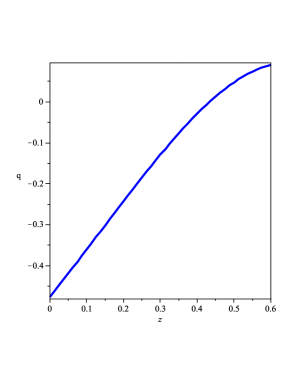
where that $\nu\neq 1$  [102]. Figure $1$ shows the behavior of $q$ versus the redshift in this model. The universe enters the accelerating phase at $z\approx 0.44$.

Figure 1: The variation of $q$ versus the redshift.

The modified Raychaudhuri equation follows easily from the Friedmann equation of the brane and the conservation of the brane energy density

$$\frac{\dot{H}}{H^{2}_{0}}=-\frac{\dot{f^{\prime}}(R,\phi)E^{2}(z)+3\Omega_{m}H_{0}(1+z)^{3}E(z)-\frac{\kappa^{2}_{4}(\dot{\rho_{c}}+\dot{\rho_{\phi}})}{3H^{2}_{0}}}{H_{0}[2f^{\prime}(R,\phi)E(z)+2\sqrt{\Omega_{r_{c}}}(1+\Omega_{\alpha}E^{2}(z))+4\sqrt{\Omega_{r_{c}}}\Omega_{\alpha}E^{2}(z)]}.$$ (24)

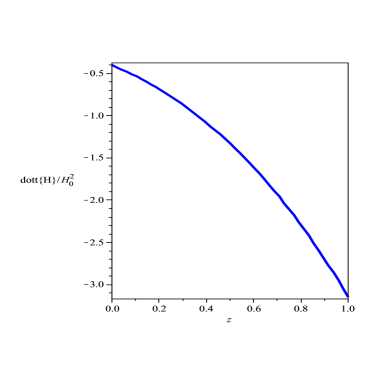
Figure $2$ shows the variation of $\frac{\dot{H}}{H^{2}_{0}}$ with redshift. It is always negative and therefore there is no super-acceleration and big-rip singularity in this braneworld scenario. Since $\dot{H}<0$, the Hubble parameter decreases as the brane expands.

Figure 2: The variation of $\frac{\dot{H}}{H^{2}_{0}}$ with redshift.

3 The Phantom-like Behavior

We will show in this section that a phantom-like behavior can be realized on the brane and this occurs without including any exotic matter that violates the null energy condition not on the brane nor in the bulk. The phantom-like behavior is based on the definition of an effective energy density which is corresponding to a balance between the cosmological constant and geometrical effects encoded on the Hubble rate evolution [36-45],[47-66]. The phantom-like behavior on the brane is based on the definition of an effective energy density $\rho_{eff}$ which increases with cosmic time and an effective equation of state parameter always less than $-1$,  $\omega_{eff}<-1$. More precisely, the effective description is inspired in writing down the modified Friedmann equation of the brane as the usual relativistic Friedmann equation so that [47-66]

$$H^{2}=\frac{\kappa^{2}_{4}}{3}(\rho_{m}+\rho_{eff}).$$ (25)

Using equations (13) and (25), we find

$$\rho_{eff}=\frac{3H^{2}_{0}}{\kappa^{2}_{4}}\bigg{[}\frac{1}{f^{\prime}(R,\phi)}\Big{[}-2\sqrt{\Omega_{r_{c}}}E(z)(1+\Omega_{\alpha}E^{2}(z))+\Omega_{m}(1+z)^{3}+\Omega_{c}+\Omega_{\phi}+\Omega_{\Lambda}\Big{]}-\Omega_{m}(1+z)^{3}\bigg{]}.$$ (26)

By definition, phantom-like prescription breaks down if $\rho_{eff}\leq 0$. Figure $3$ shows the variation of $\rho_{eff}$ versus $z$ in our proposed setup.

Figure 3: $\rho_{eff}$ versus redshift.

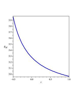
It is always positive and grows with cosmic time, therefore effective energy density shows the phantom-like behavior. In this respect, the important feature of this scenario is the fact that this phantom-like behavior never breaks down at least in the proposed subspace of the model parameter space. Nevertheless, there are other subspaces of the model parameter space that phantom-like prescription may be broken in these subspaces in the same way as has been mentioned by Bouhamdi-Lopez in Ref. [47-66]. The main point here is the fact that it is possible essentially to save phantom-like prescription for a wide range of redshifts.

The effective equation of state parameter $\omega_{eff}$, can be defined using the conservation equation of the effective energy density on the brane

$$\dot{\rho}_{eff}+3H(1+\omega_{eff})\rho_{eff}=0.$$ (27)

The effective energy density evolve as follows

$$\dot{\rho}_{eff}=\frac{-3}{\kappa^{2}_{4}}\bigg{[}\frac{[2\dot{H}H_{0}\sqrt{\Omega_{r_{c}}}(1+\Omega_{\alpha}E^{2}(z))+2\Omega_{\alpha}E^{2}(z)\dot{H}H_{0}+3\Omega_{m}E(z)(1+z)^{3}H^{3}_{0}-\frac{\kappa^{2}_{4}\dot{\rho}_{c}+\dot{\rho}_{\phi}}{3}]}{f^{\prime}(R,\phi)}$$

$$+\frac{\dot{f^{\prime}}(R,\phi)H^{2}_{0}[-2\sqrt{\Omega_{r_{c}}}(1+\Omega_{\alpha}E^{2}(z))+\Omega_{m}(1+z)^{3}+\Omega_{c}+\Omega_{\phi}+\Omega_{\Lambda}]}{(f^{\prime}(R,\phi))^{2}}-3\Omega_{m}(1+z)^{3}E(z)H^{3}_{0}\bigg{]}.$$ (28)

By defining

$$y\equiv\frac{\dot{f^{\prime}}(R,\phi)H^{2}_{0}[-2\sqrt{\Omega_{r_{c}}}(1+\Omega_{\alpha}E^{2}(z))+\Omega_{m}(1+z)^{3}+\Omega_{c}+\Omega_{\phi}+\Omega_{\Lambda}]}{(f^{\prime}(R,\phi))^{2}}-3\Omega_{m}(1+z)^{3}E(z)H^{3}_{0},$$ (29)

we find

$$1+\omega_{eff}=\frac{\frac{-3}{\kappa^{2}_{4}}[\frac{[2\dot{H}H_{0}\sqrt{\Omega_{r_{c}}}(1+\Omega_{\alpha}E^{2}(z))+2\Omega_{\alpha}E^{2}(z)\dot{H}H_{0}+3\Omega_{m}E(z)(1+z)^{3}H^{3}_{0}-\frac{\kappa^{2}_{4}\dot{\rho}_{c}+\dot{\rho}_{\phi}}{3}]}{f^{\prime}(R,\phi)}+y]}{3H_{0}E(z)\rho_{eff}}.$$ (30)

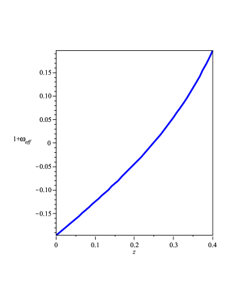
Figure $4$ shows the plot of $1+\omega_{eff}$ versus the redshift. The universe enters to the phantom phase in $z\approx 0.25$. As this figure shows, the phantom-like behavior has no break down at small redshifts in contrast to the $\Lambda$DGP-GB model [47-66]. So, our model realizes a phantom-like behavior without introducing any phantom matter on the brane or in the bulk. It is important to note that this setup explains also a smooth transition to phantom phase, the so called phantom-divide line crossing.

Figure 4: $1+w_{eff}$ versus the redshift.

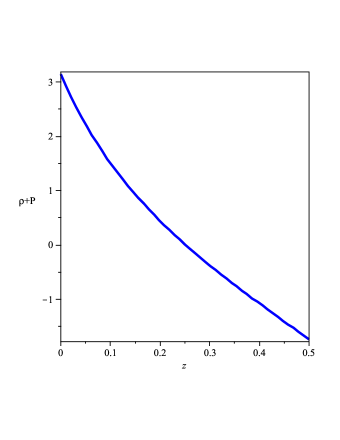
Our main achievement here is the realization of the phantom-like behavior without introducing any phantom matter not on the brane nor in the bulk. Nevertheless, the phantom-like behavior realized in this gravitational way should respect the null energy condition, at least in some subspaces of the model parameter space. So, we should check the status of the null energy condition in this setup. The null energy condition is respected if $\rho_{eff}+p_{eff}>0$. Figure $5$ shows a plot of $\rho_{eff}+p_{eff}$ versus the redshift. As this figure shows, the phantom-like behavior in our proposed model occurs without violation of the null energy condition at least in some subspaces of the model parameter space. Especially, this condition is respected in the phantom-like region of the model. We emphasize that validity of the null energy condition in the phantom-like region of the scenario is important for our purposes in this paper. This is because with phantom fields usually the null energy condition breaks down. Here we realized a phantom-like behavior in a braneworld setup without violation of the null energy condition in the phantom-like region. It is important to note that in the non-phantom region, the situation is different and the validity of null energy condition is guaranteed by positivity of the effective energy density in this region.

Figure 5: The status of the null energy condition in this setup: $\rho_{eff}+p_{eff}$ versus the redshift.

4 Lue-Starkman Screening of the Brane Cosmological Constant

Lue and Starkman have shown that one can realize phantom-like effect, that is, increasing of the effective dark energy density with redshift, in the normal branch of the DGP cosmological solution without introducing any phantom field [103]. The normal branch of the DGP model which cannot explain the self-acceleration, has the key property that brane is extrinsically curved so that shortcuts through the bulk allow gravity to screen the effects of the brane energy-momentum contents at Hubble parameters $H\sim r_{c}^{-1}$ where $r_{c}$ is the crossover distance [103]. Since in this case $H(z)$ is a decreasing function of the redshift, the effective dark energy component is increasing with redshift and therefore we observe a phantom-like behavior without introducing any phantom matter that violates the null energy condition and suffers from several theoretical problems. In the first step, in this section we study the phantom-like effect in the normal branch of a GBIG scenario. In other words, here we suppose that there is a quintessence field non-minimally coupled to modified induced gravity on the brane in addition to a Gauss-Bonnet term in the bulk action. In fact we incorporate the possibility of modification of the induced gravity on the brane in the spirit of $f(R)$ gravity. We emphasize also that we have included a canonical (quintessence) scalar field to incorporate possible coupling of the gravity and scalar degrees of freedom on the brane. This provides a wider parameter space with capability to handle the problem more completely. In fact, inclusion of this quintessence field brings the theory to realize crossing of the phantom divide line [36-40]. Considering the normal branch of the equation (13) , we have

$$H^{2}=\frac{8\pi G}{3}(\rho_{m}+\rho_{\phi}+\rho_{c})+\frac{\Lambda}{3}-\frac{[f^{\prime}(R,\phi)]^{-1}H}{r_{c}}(1+\frac{8}{3}\alpha H^{2}),$$ (31)

where $G\equiv G_{eff}=\Big{(}8\pi M_{4}^{2}F^{\prime}(R,\phi)\Big{)}^{-1}$ and a prime denotes differentiation with respect to $R$. Now, we rewrite this equation in the following form

$$H^{2}=\frac{8\pi G}{3}(\rho_{m}+\rho_{\phi}+\rho_{c})+\frac{8\pi G}{3}(\rho_{DE}^{eff}).$$ (32)

By comparing this equation with the Friedmann equation (31), we find

$$\frac{8\pi G}{3}(\rho_{DE}^{eff})=\frac{\Lambda}{3}-\frac{[f^{\prime}(R,\phi)]^{-1}H}{r_{c}}(1+\frac{8}{3}\alpha H^{2}).$$ (33)

As a result, in this GBIG-inspired model the crossover scale takes the following form

$$r_{f}=\frac{M_{4}^{2}f^{\prime}(R,\phi)}{2M_{5}^{3}}={f^{\prime}(R,\phi)r_{c}},$$ (34)

Now as an enlightening example, we set for instance

$$f(R,\phi)=\Big{(}R-R_{c}\frac{\alpha_{0}(\frac{R}{R_{c}})^{n}}{1+\beta_{0}(\frac{R}{R_{c}})^{n}}\Big{)}\Big{(}\frac{1}{2}(1-\xi\phi^{2})\Big{)}\Big{.}$$ (35)

where the $f(R)$ part is the Hu-Sawicki model [25]. With this choice, one recovers the general relativity for $n=0$. For $n\neq 0$, we obtain

$$\frac{8\pi G}{3}(\rho_{DE}^{eff})=\frac{\Lambda}{3}-\frac{[\Big{(}R-R_{c}\frac{\alpha_{0}(\frac{R}{R_{c}})^{n}}{1+\beta_{0}(\frac{R}{R_{c}})^{n}}\Big{)}\Big{(}\frac{1}{2}(1-\xi\phi^{2})\Big{)}]^{-1}H}{r_{c}}(1+\frac{8}{3}\alpha H^{2})\,,$$ (36)

where for a spatially flat FRW geometry, the Riici scalar is given by

$$R=6\frac{\ddot{a}}{a}+6(\frac{\dot{a}}{a})^{2}.$$ (37)

Figure $6$ shows the variation of $\rho_{eff}^{DE}$ versus $n$ and the redshift in this GBIG-inspired $F(R,\phi)$ model. As we see, the phantom-like behavior can be realized for all values of $n$ constraint in the Hu-Sawicki model. In other words, for all values of acceptable $n$ in the Hu-Sawicki model, the effective dark energy in this GBIG-inspired $F(R,\phi)$ model has the phantom-like behavior.

Figure 6: Variation of the effective dark energy density versus $n$ and $z$ in a GBIG-inspired $F(R,\phi)$ model with $F(R,\phi)=f(R,\phi)=\Big{(}R-R_{c}\frac{\alpha_{0}(\frac{R}{R_{c}})^{n}}{1+\beta_{0}(\frac{R}{R_{c}})^{n}}\Big{)}\Big{(}\frac{1}{2}(1-\xi\phi^{2})\Big{)}$. The phantom-like behavior can be realized for all $n$.

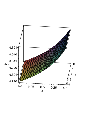
Figure $7$ shows the variation of the effective dark energy density versus $z$ and the non-minimal coupling. By increasing the values of $\xi$, the effective dark energy density reduces, and for a fixed value of $\xi$ there is phantom-like effect for appropriate values of $n$.

Figure 7: Variation of the effective dark energy density versus $z$ and the non-minimal coupling.

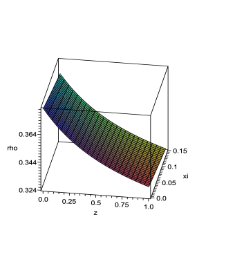
Also, figure $8$ shows the variation of the effective dark energy density versus $n$ and the non-minimal coupling. The phantom-like effect ( increasing the values of the effective dark energy density with cosmic time) can be realized for suitable ranges of $n$ and $\xi$.

Figure 8: Variation of the effective dark energy density versus $n$ and the non-minimal coupling.

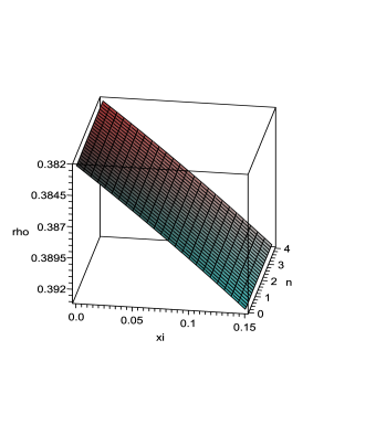
As an important especial case, for $F(R,\phi)=f(R)$ we find the screening effect in a general GBIG $f(R)$-gravity

$$\frac{8\pi G}{3}\rho_{DE}^{eff}=\lambda-\frac{\Big{[}f^{\prime}(R)\Big{]}^{-1}H}{r_{c}}(1+\frac{8}{3}\alpha H^{2}).$$ (38)

Now as an enlightening example, we set for instance

$$f(R)=\Big{(}R-R_{c}\frac{\alpha_{0}(\frac{R}{R_{c}})^{n}}{1+\beta_{0}(\frac{R}{R_{c}})^{n}}\Big{)}$$ (39)

Figure $9$ shows the variation of the effective dark energy density versus $n$. There is phantom-like effect for all possible values of $n$ in the Hu-Sawicki model.

Figure 9: variation of the $\rho_{DE}$ versus n.

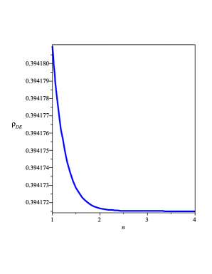
Figure $10$ shows the variation of the effective dark energy density versus the redshift.

Figure 10: : $\rho_{DE}$ versus the redshift.

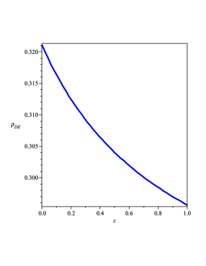
The main result of these numerical solutions is that this modified GBIG scenario has the capability to realize the phantom-like prescription without introducing any phantom field neither on the brane nor in the bulk. We note that we have included a quintessence field non-minimally coupled to the modified induced gravity on the brane to have a wider parameter space and to include all possible situations.

5 Dynamical Screening and Phantom-Like Mimicry with non-minimal coupling and curvature effect

Our setup in this section contains a DGP-inspired braneworld scenario with curvature effect through the Gauss-Bonnet term in the bulk action and a non-minimally coupled scalar field on the brane. The ordinary matter localized on the brane is assumed to be a quintessence scalar field non-minimally coupled to the induced gravity on the brane. This canonical scalar field respects the null energy condition and we assume there is no phantom matter present on the brane or in the bulk. By virtue of dynamical screening, we show that this model accounts for a phantom-like behavior without violating the null energy condition. In addition, we show that in contrast to existing literature which argued that this phantom-like effect breaks down in some small values of redshift, there is no break-down of this behavior in the presence of the non-minimal coupling of the quintessence field . The action of our model with Gauss-Bonnet and induced gravity effects and a scalar field non-minimally coupled to induced gravity on the brane is given as follows [104] (see also [81-84])

$$S=\frac{1}{2\kappa_{5}^{2}}\int d^{5}x\sqrt{-g^{(5)}}\Bigg{[}R^{(5)}-2\Lambda_{5}+\alpha\Big{(}R^{(5)2}-4R_{ab}^{(5)}R^{(5)ab}+R_{abcd}^{(5)}R^{(5)abcd}\Big{)}\Bigg{]}$$

$$+\Bigg{[}\frac{r_{c}}{2\kappa_{5}^{2}}\int d^{4}x\sqrt{-g}\bigg{(}\beta(\phi)R-2\kappa_{4}^{2}g^{\mu\nu}\nabla_{\mu}\phi\nabla_{\nu}\phi-4\kappa_{4}^{2}V(\phi)-4\kappa_{4}^{2}\lambda\bigg{)}\Bigg{]}_{y=0},$$ (40)

where $\alpha$ and $r_{c}$ are the GB coupling constant and IG cross-over scale respectively. We assume the brane is located at $y=0$ where $y$ is the coordinate of the extra dimension. Also $\beta(\phi)$ is a general non-minimal coupling of the scalar field and induced gravity on the brane. The cosmological dynamics of the model is given by the following generalized Friedmann equation [104]

$$\bigg{[}1+\frac{8}{3}\alpha\Big{(}H^{2}+\frac{\Phi}{2}+\frac{K}{a^{2}}\Big{)}\bigg{]}^{2}\Big{(}H^{2}-\Phi+\frac{K}{a^{2}}\Big{)}=\bigg{[}r_{c}\beta(\phi)H^{2}+r_{c}\beta(\phi)\frac{K}{a^{2}}-\frac{k^{2}_{5}}{6}\Big{(}\rho+\rho_{\phi}+\lambda\Big{)}\bigg{]}^{2}.$$ (41)

This equation describes the cosmological evolution on the brane with tension and a non-minimally coupled scalar field localized on the brane. As usual, the bulk contains a black hole mass and a cosmological constant, so that $\Phi$ is defined as equation (12). As usual, $r_{c}$ is the crossover scale in the DGP model and $\alpha$ measures the strength of the GB curvature effect on the brane. If $\alpha=0$, the model reduces to the DGP model with a non-minimally coupled scalar field on the brane, while for $r_{c}=0$ we recover the Gauss-Bonnet braneworld model. Here, we restrict our study to the case where the bulk black hole mass vanishes and we neglect the bulk cosmological constant too ( that is, $\Lambda_{5}=0$). For a spatially flat FRW brane, the Friedmann equation is given by

$$\bigg{[}1+\frac{8}{3}\alpha\Big{(}H^{2}+\frac{\Phi}{2}\Big{)}\bigg{]}^{2}(H^{2}-\Phi)=\bigg{[}r_{c}\beta(\phi)H^{2}-\frac{\kappa^{2}_{5}}{6}\Big{(}\rho+\rho_{\phi}+\lambda\Big{)}\bigg{]}^{2}.$$ (42)

We restrict ourselves to the normal branch of this GBIG-inspired scenario and therefore there is no ghost instabilities in this case. The energy density on the brane $\rho$, is composed of a CDM component ( with energy density $\rho_{m}$ ) and a cosmological constant $\Lambda_{4}$

$$\rho=\rho_{m}+\Lambda_{4}.$$ (43)

Considering the normal branch of the equation (43), we have

$$H^{2}=\frac{8\pi G}{3}(\rho_{m}+\rho_{\phi})+\frac{\Lambda_{4}}{3}-\frac{[\beta(\phi)]^{-1}H}{r_{c}}(1+\frac{8}{3}\alpha H^{2}).$$ (44)

Comparing this equation with the following Friedmann equation

$$H^{2}=\frac{8\pi G}{3}(\rho_{m}+\rho_{\phi})+\frac{8\pi G}{3}(\rho_{DE}^{eff})$$ (45)

we find

$$\frac{8\pi G}{3}(\rho_{DE}^{eff})=\frac{\Lambda_{4}}{3}-\frac{[\beta(\phi)]^{-1}H}{r_{c}}(1+\frac{8}{3}\alpha H^{2})$$ (46)

where $G\equiv G_{eff}=\Big{(}8\pi M_{5}^{2}\beta(\phi)\Big{)}^{-1}$ and the crossover scale takes the following form

$$r_{f}=\frac{M_{4}^{2}\beta(\phi)}{2M_{5}^{3}}={\beta(\phi)r_{c}}.$$ (47)

Equation (46) shows the dynamical screening of the brane cosmological constant due to both non-minimal coupling and the Gauss-Bonnet effect. In which follows, we set for simplicity $\beta(\phi)=\frac{1}{2}(1-\xi\phi^{2})$ where $\xi$ is the conformal coupling. We note also that in our numerical calculations we adopt the ansatz $\phi(t)=\phi_{0}t^{-\mu}$ and $a(t)=\Big{(}t^{2}+\frac{t_{0}}{1-\nu}\Big{)}^{\frac{1}{1-\nu}}$, where $\mu$ and $\nu$ are positive constants. We obtain from equation (46)

$$\frac{8\pi G}{3}(\rho_{DE}^{eff})=\frac{\Lambda_{4}}{3}-\frac{[\Big{(}\frac{1}{2}(1-\xi\phi^{2})\Big{)}]^{-1}H}{r_{c}}(1+\frac{8}{3}\alpha H^{2}).$$ (48)

Figure $11$ shows the variation of $\rho_{DE}^{eff}$ versus $\xi$ in a constant time slice. The range of $\xi$ are chosen from [67-71] constraint by the recent observations. As this figure shows, by increasing the values of the nonminimal coupling, $\rho_{DE}^{eff}$ decreases in a fixed redshift( fixed time slice).

Figure 11: $\rho_{DE}^{eff}$ versus $\xi$ in a constant time slice.

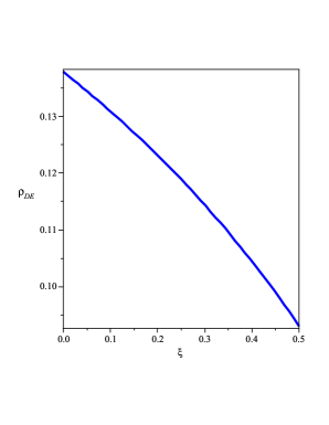
Figure $12$ shows the variation of the effective dark energy density versus the redshift. As this figure shows, $\rho_{DE}^{eff}$ increases by decreasing the redshift and this is exactly the phantom-like behavior we are interested in. Note that this phantom-like effects is realized without introducing any phantom matter on the brane and only screening of the brane cosmological constant due to non-minimal coupling and the curvature effect causes such an intriguing aspect.

Figure 12: $\rho_{DE}$ versus redshift.

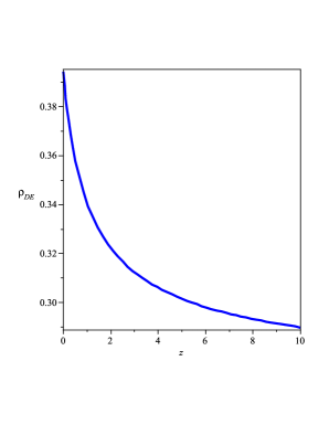
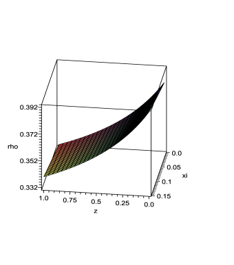
Figure $13$ shows the variation of the effective dark energy density versus the redshift and the non-minimal coupling. We note that while the introduction of a phantom field requires the violation of the null energy condition, here this energy condition is respected ( at least in some subspaces of the model parameter space) since we have not included any phantom matter on the brane. In other words, since the phantom-like dynamics realized in this setup is gravitational ( the quintessence field introduced on the brane plays the role of standard matter on the brane), the null energy condition could be respected in some subspaces of the model parameter space.

Figure 13: Variation of the effective dark energy versus the redshift and the non-minimal coupling.

6 Conclusion

In this paper we have analyzed in some detail a modified $\Lambda$DGP-Gauss-Bonnet model which corresponds to a 5D braneworld model where the bulk is a 5D Minkowski space-time. This model contains a Gauss-Bonnet term in the bulk and an induced gravity term on the brane which is modified in the spirit of $f(R)$ gravity. We incorporated also a canonical (quintessence) scalar field non-minimally coupled to induced gravity on the brane. Our analysis is performed for the normal (or non self-accelerating) ghost-free branch which we have assumed to be filled by cold deark matter (CDM) and a cosmological constant. We have shown especially that how the brane accelerates at late-time in this normal branch. An interesting feature of this model is the role played by the extra dimension: it induces a mimicry of a phantom-like behavior without introducing any matter that violates the null energy condition on the brane. This phantom-like behavior happens without any super-acceleration of the brane. We should emphasize that the Gauss-Bonnet effect which induces the ultraviolet corrections on the brane, modifies the phantom-like behavior at earlier times. Therefore, a consistent DGP brane model which essentially is an infra-red modification of the General Relativity, should have ultraviolet modifications as well and this is achieved by incorporation of the Gauss-Bonnet term in the bulk action. We have incorporated also the possible modification of the induced gravity on the brane. This is equivalent to introduce a canonical scalar field on the brane with General Relativity as the background gravitational theory. By adopting suitable and observationally viable ansatz for $f(R,\phi)$ and the scale factor, we have shown that this model realizes the phantom-like behavior in some subspaces of the model parameter space without violation of the null energy condition. The phantom-like prescription in our proposed model has no break down in some appropriate subspaces of the model parameter space and it realizes a smooth crossing of the phantom-divide line.

Acknowledgment
This work has been supported partially by Research Institute for Astronomy and Astrophysics of Maragha, IRAN.

References

- [1] S. Perlmutter et al, Astrophys. J. 517 (1999) 565
- [2] A. G. Riess et al, Astron. J. 116 (1998) 1006
- [3] A. D. Miller et al, Astrophys. J. Lett. 524 (1999) L1
- [4] P. de Bernardis et al, Nature 404 (2000) 955
- [5] S. Hanany et al, Astrophys. J. Lett. 545 (2000) L5
- [6] D. N. Spergel et al, Astrophys. J. Suppl. 148 (2003) 175
- [7] L. Page et al, Astrophys. J. Suppl. 148 (2003) 233
- [8] G. Hinshaw et al, [WMAP Collaboration], arXiv:0803.0732
- [9] D. N. Spergel et al, Astrophys. J. Suppl. 170 (2007) 377
- [10] G. Hinshaw et al, Astrophys. J. Suppl. 170 (2007) 288
- [11] L. Page et al, Astrophys. J. Suppl. 170 (2007) 335
- [12] T. Padmanabhan, Phys. Rept. 380 (2003) 235
- [13] I. Fujii, K. Maeda, The scalar - tensor theory of gravity, Cambridge University Press, Cambridge (UK), 2003
- [14] P. Caresia, S. Matarrese and L. Moscardini, Astrophys. J. 605, 21 (2004)
- [15] V. Pettorino, C. Baccigalupi and G. Mangano, JCAP 0501, 014 (2005).
- [16] S. Nojiri and S. D. Odintsov, Int. J. Geom. Meth. Mod. Phys. 4, 115 (2007) [arXiv:hep-th/0601213]
- [17] S. Capozziello and M. Francaviglia, Gen. Rel. Grav. 40, 357 (2008) [arXiv:0706.1146 [astro-ph]]
- [18] T. P. Sotiriou and V. Faraoni, [arXiv:0805.1726 [gr-qc]].
- [19] H. Kleinert and H.-J. Schmidt, Gen. Rel. Grav. 34, 1295 (2002)
- [20] S. Nojiri and S.D. Odintsov, Phys. Lett. B, 576, 5 (2003)
- [21] S. Nojiri and S.D. Odintsov, Mod. Phys. Lett. A, 19, 627 (2003)
- [22] S. Nojiri and S.D. Odintsov, Phys. Rev. D, 68, 12352 (2003)
- [23] S.M. Carroll, V. Duvvuri, M. Trodden and M. Turner, Phys. Rev. D, 70, 043528 (2004)
- [24] G. Allemandi, A. Borowiec and M. Francaviglia, Phys. Rev. D 70, 103503 (2004)
- [25] W. Hu and I. Sawicki, Phys. Rev. D 76, 064004 (2007) [arXiv:0705.1158].
- [26] A. A. Starobinsky, JETP Lett. 86, 157 (2007) [arXiv:0706.2041].
- [27] S. A. Appleby and R. A. Battye, Phys. Lett. B 654, 7 (2007).
- [28] S. Nojiri and S. D. Odintsov, Phys. Lett. B 652, 343 (2007) [arXiv:0706.1378].
- [29] S. Nojiri and S. D. Odintsov, Phys. Rev. D 78, 046006 (2008) [arXiv:0804.3519]
- [30] S. Nojiri and S. D. Odintsov, AIP Conf. Proc. 1115, (212) (2009) [arXiv:0810.1557]
- [31] G. Cognola, E. Elizalde, S. Nojiri, S. D. Odintsov, L. Sebastiani and S. Zerbini, Phys. Rev. D 77, 046009 (2008) [arXiv:0712.4017].
- [32] G. Dvali, G. Gabadadze and M. Porrati, Phys. Lett. B 485 (2000) 208, [hep-th/0005016]
- [33] C. Deffayet, Phys. Lett. B 502, 199 (2001)
- [34] C. Deffayet, G. Dvali and G. Gabadadze, Phys. Rev. D 65, 044023 (2002)
- [35] C. Deffayet, S. J. Landau, J. Raux, M. Zaldarriaga and P. Astier, Phys. Rev. D 66, 024019 (2002).
- [36] V. Sahni and Y. Shtanov, JCAP 0311, 014 (2003) [arXiv:astro-ph/0202346]
- [37] V. Sahni [arXiv:astro-ph/0502032]
-
[38]
R. Lazkoz, R. Maartens and E. Majerotto, Phys. Rev. D 74,
083510 (2006) [arXiv:astro-ph/0605701]
- [39] L. P. Chimento, R. Lazkoz, R. Maartens and I. Quiros, JCAP 0609 (2006) 004, [arXiv:astro-ph/0605450]
- [40] R. Maartens and E. Majerotto [arXiv:astro-ph/0603353].
- [41] K. Nozari and F. Kiani, JCAP 07 (2009) 010, [ arXiv:0906.3806]
- [42] M. Bouhmadi-Lopez, [arXiv:0905.1962]
- [43] K. Nozari and N. Rashidi, JCAP 0909 (2009) 014, [arXiv:0906.4263]
- [44] K. Nozari, T. Azizi and M. R. Setare, JCAP 10 (2009) 022, [arXiv:0910.0611]
- [45] K. Nozari and T. Azizi, Phys. Lett. B 680 (2009) 205, [arXiv:0909.0351].
- [46] K. Koyama, Class. Quant. Grav. 24, R231 (2007) [arXiv:0709.2399 [hep-th]].
- [47] M. Bouhmadi-Lopez, Nucl. Phys. B 797, 78 (2008) [arXiv:astro-ph/0512124]
- [48] M. Bouhmadi-Lopez and P. V. Moniz, Phys. Rev. D 78, 084019 (2008) [arXiv:0804.4484]
- [49] M. Bouhmadi-Lopez and P. V. Moniz, AIP Conf. Proc. 1122, 201 (2009) [arXiv:0905.4269]
- [50] A. Vikman, Phys. Rev. D 71 (2005) 023515, [astro-ph/0407107]
- [51] Y. H. Wei and Y. Z. Zhang, Grav. Cosmol. 9 (2003) 307
- [52] V. Sahni and Y. Shtanov, JCAP 0311 (2003) 014
- [53] Y. H. Wei and Y. Tian, Class. Quantum Grav. 21 (2004) 5347
- [54] F. C. Carvalho and A. Saa, Phys. Rev. D 70 (2004) 087302
- [55] F. Piazza and S. Tsujikawa, JCAP 0407 (2004) 004
- [56] R. G. Cai, H. S. Zhang and A.Wang, Commun. Theor. Phys. 44 (2005) 948
- [57] I. Y. Arefeva, A. S. Koshelev and S. Y. Vernov, Phys. Rev. D 72 (2005) 064017
- [58] A. Anisimov, E. Babichev and A. Vikman, JCAP 0506 (2005)006
- [59] B. Wang, Y.G. Gong and E. Abdalla, Phys. Lett. B 624 (2005) 141
- [60] S. Nojiri and S. D. Odintsov, [hep-th/0506212]
- [61] S. Nojiri, S. D. Odintsov and S. Tsujikawa, [hep-th/0501025]
- [62] E. Elizalde, S. Nojiri, S. D. Odintsov and P. Wang, Phys. Rev. D 71 (2005) 103504
- [63] W. Zhao and Y. Zhang, Phys. Rev.D 73 (2006) 123509
- [64] P. S. Apostolopoulos and N. Tetradis, [hep-th/0604014]
- [65] I. Ya. Arefeva and A. S. Koshelev, [hep-th/0605085]
- [66] S. D. Sadatian and K. Nozari, Europhys. Lett. 82 (2008) 49001.
- [67] R. Gannouji, D. Polarski, A. Ranquet and A. A. Starobinsky, JCAP 0609 (2006) 016, [arXiv:astro-ph/0606287]
- [68] O. Hrycyna and M. Szydlowski, Phys. Lett. B651 (2007) 8, [arXiv:0704.1651]
- [69] O. Hrycyna and M. Szydlowski, Phys. Rev. D76 (2007) 123510, [arXiv:0707.4471]
- [70] M. Szydlowski, O. Hrycyna and A. Kurek, Phys. Rev. D 77 (2008) 027302, [arXiv:0710.0366]
- [71] S. Nojiri, S. D. Odintsov and P. V. Tretyakov, [ arXiv:0710.5232]
- [72] S. Capozziello, V. F. Cardone and A. Troisi, JCAP 0608 (2006) 001, [arXiv:astroph/ 0602349]
- [73] S. Capozziello, S. Nojiri and S.D. Odintsov, Phys. Lett. B 634 (2006) 93, [arXiv:hep-th/0512118]
- [74] S. Capozziello, V. F. Cardone, E. Piedipalumbo and C. Rubano, Class. Quant. Grav. 23 (2006) 1205, [arXiv:astro-ph/0507438]
- [75] S. Capozziello, V. F. Cardone, S. Carloni and A. Troisi, Int. J. Mod. Phys. D12 (2003) 1969, [arXiv:astro-ph/0307018].
- [76] K. Atazadeh, M. Farhoudi and H. R. Sepangi, Phys. Lett. B 660 (2008) 275, [arXiv:0801.1398]
- [77] K. Atazadeh and H. R. Sepangi, JCAP 09 (2007) 020, [arXiv:0710.0214].
- [78] S. Nesseris and L. Perivolaropoulos, JCAP 0701 (2007) 018; [arXiv:astro-ph/0610092].
- [79] H. Zhang and Z.-H. Zhu, Phys. Rev. D 75 (2007) 023510, [arXiv:astro-ph/0611834]
- [80] K. Nozari, N. Behrouz, T. Azizi and B. Fazlpour, Prog. Theor. Phys. Vol. 122, No. 3 (2009) [arXiv:0808.0318].
- [81] R. A. Brown, [arXiv:gr-qc/0701083]
- [82] R. A. Brown et al, JCAP 0511, 008 (2005), [arXiv:gr-qc/0508116]
- [83] K. Nozari and B. Fazlpour, JCAP 0806, (032) (2008) [ arXiv:0805.1537]
- [84] B. Gumjudpai, Gen. Relat.Gravit. 36, 747 (2004).
- [85] R.-G. Cai, H.-S. Zhang and A. Wang, Commun. Theor. Phys. 44, 948 (2005) [arXiv:hep-th/0505186]
- [86] S. Nojiri, S. D. Odintsov and P. V. Tretyakov, Phys. Lett. B 651 224 (2007) [arXiv:0704.2520]
- [87] G. Cognola, E. Elizalde, S. Nojiri, S. D. Odintsov and S. Zerbini, Phys. Rev. D 73, 084007 (2006) [arXiv:hep-th/0601008]
- [88] S. Nojiri and S. D. Odintsov, Phys. Lett. B 631, 1 (2005) [arXiv:hep-th/0508049]
- [89] S. Nojiri, S. D. Odintsov and M. Sasaki, Phys. Rev. D71, 123509 (2005) [arXiv:hep-th/0504052].
- [90] P. S. Apostolopoulos, N. Brouzakis, N. Tetradis and E. Tzavara, Phys. Rev.D 76 (2007) 084029, [arXiv:0708.0469].
- [91] R. Dick, Class. Quant. Grav. 18 (2001) R1-R24, [arXiv:hep-th/0105320]
- [92] K. Nozari, JCAP 0709 (2007) 003, [arXiv:0708.1611]
- [93] K. Nozari and M. Pourghassemi, JCAP 10 044 (2008) [arXiv:0808.3701]
- [94] K. Nozari, JCAP, 09 003 (2007) [arXiv:hep-th/07081611]
- [95] K. Atazadeh and H. R. Sepangi, Phys. Lett. B 643 76 (2006) [arXiv:gr-qc/0610107]
- [96] K. Atazadeh and H. R. Sepangi, JCAP 0709 020 (2007) [ arXiv:0710.0214]
- [97] K. Atazadeh and H. R. Sepangi, JCAP 01 006 (2009) [arXiv:0811.3823]
- [98] J. Saavedra and Y. Vasquez, [arXiv:0803.1823].
- [99] A. D. Dolgov and M. Kawasaki, Phys. Lett. B573 (2003) 1, [arXiv:astro-ph/0307285]
- [100] C. -G. Shao, R.-G. Cai, B. Wang and R.-K. Su, Phys. Lett. B633 (2006) 164, [arXiv:gr-qc/0511034]
- [101] A. L. Erickcek, T. L. Smith and M. Kamionkowski, Phys. Rev.D74 (2006) 121501, [arXiv:astro-ph/0610483].
- [102] Y.-Fu. Cai, T. Qiu, Y.-S. Piao, M. Li and X. Zhang, JHEP 0710 (2007) 071, [arXiv:0704.1090]
- [103] A. Lue and G. D. Starkman, Phys. Rev. D 70 (2004) 101501, [arXiv:astro-ph/0408246]
- [104] K. Nozari and B. Fazlpour, JCAP 06 (2008) 032, [arXiv:0805.1537]