Re-Pair Compression of Inverted Lists

Abstract

Compression of inverted lists with methods that support fast intersection operations is an active research topic. Most compression schemes rely on encoding differences between consecutive positions with techniques that favor small numbers. In this paper we explore a completely different alternative: We use Re-Pair compression of those differences. While Re-Pair by itself offers fast decompression at arbitrary positions in main and secondary memory, we introduce variants that in addition speed up the operations required for inverted list intersection. We compare the resulting data structures with several recent proposals under various list intersection algorithms, to conclude that our Re-Pair variants offer an interesting time/space tradeoff for this problem, yet further improvements are required for it to improve upon the state of the art.

1 Introduction

Inverted indexes are one of the oldest and simplest data structures ever invented, and at the same time one of the most successful ones in Information Retrieval (IR) for natural language text collections. They play a central role in any book on the topic [BYR99, WMB99], and are also at the heart of most modern Web search engines, where simplicity is a plus.

An inverted index is a vector of lists. Each vector entry corresponds to a different word or term, and its list points to the occurrences of that word in the text collection. The collection is seen as a set of documents. The set of different words is called the vocabulary. Empirical laws well accepted in IR [Hea78] establish that the vocabulary is much smaller than the collection size $n$, more precisely of size $O(n^{\beta})$, for some constant $0<\beta<1$ that depends on the text type.

Two main variants of inverted indexes exist [BYMN02, ZM06]. One is aimed at retrieving documents which are “relevant” to a query, under some criterion. Documents are regarded as vectors, where terms are the dimensions, and the values of the vectors correspond to the relevance of the terms in the documents. The lists point to the documents where each term appears, storing also the weight of the term in that document (i.e., the coordinate value). The query is seen as a set of words, so that retrieval consists in processing the lists of the query words, finding the documents which, considering the weights the query terms have in the document, are predicted to be relevant. Query processing usually involves somehow merging the involved lists, so that documents can get the combined weights over the different terms. Algorithms for this type of queries have been intensively studied, as well as different data organizations for this particular task [PZSD96, WMB99, ZM06, AM06, SC07]. List entries are usually sorted by descending relevance of the term in the documents.

The second variant, which is our focus, are the inverted indexes for so-called full-text retrieval. These are able of finding the documents where the query appears. In this case the lists point to the documents where each term appears, usually in increasing document order. Queries can be single words, in which case the retrieval consists simply of fetching the list of the word; or disjunctive queries, where one has to fetch the lists of all the query words and merge the sorted lists; or conjunctive queries, where one has to intersect the lists. While intersection can be done also by scanning all the lists in synchronization, it is usually the case that some lists are much shorter than the others [Zip49], and this opens many opportunities of faster intersection algorithms. Those are even more relevant when many words have to be intersected.

Intersection queries have become extremely popular because of Google-like default policies to handle multiword queries. Given the huge size of the Web, Google solves the queries, in principle, by intersecting the inverted lists. Another important query where intersection is essential is the phrase query. This can be solved by intersecting the documents where the words appear and then postprocessing the candidates. In order to support phrase queries at the index level, the inverted index must store all the positions where each word appears in each document. Then phrase queries can be solved essentially by intersecting word positions. The same opportunities for smart intersection arise.

The amount of recent research on intersection of inverted lists witnesses the importance of the problem [DM00, BK02, BY04, BYS05, BLOL06, ST07, CM07]. Needless to say, space is an issue in inverted indexes, especially if one has to store word positions. Much research has been carried out on compressing inverted lists [WMB99, NMN⁺00, ZM06, CM07], and on its interaction with the query algorithms, including list intersections. Despite that algorithms in main memory have received much attention, in many cases one resorts to secondary memory, which brings new elements to the tradeoffs. Compression not only reduces space, but also transfers from secondary memory when fetching inverted lists (the vocabulary usually fits in main memory even for huge text collections). Yet, the random accesses used by the smart intersection algorithms become more expensive.

Most of the list compression algorithms rely on the fact that the inverted lists are increasing, and that the differences between consecutive entries are smaller on the longer lists. Thus, a scheme that represents those differences with encodings that favor small numbers work well [WMB99]. Random access is supported by storing sampled absolute values, and some storage schemes for those samples considering secondary storage have been proposed as well [CM07].

In this paper we explore a completely different compression method for inverted lists: We use Re-Pair compression of the differences. Re-Pair [LM00] is a grammar-based compression method that generates a dictionary of common sequences, and then represents the data as a sequence of those dictionary entries. It is simple and fast at decompression, allowing for efficient random access to the data even on secondary memory, and achieves competitive compression ratios. It has been successfully used for compression of Web graphs [CN07], where the adjacency lists play the role of inverted lists. Using it for inverted lists is more challenging because several other operations must be supported apart from fetching a list, in particular the many algorithms for list intersection. We show that Re-Pair is well-suited for this task as well, and also design new variants especially tailored to the various intersection algorithms. We test our techniques against a number of the best existing compression methods and intersection algorithms, showing that our Re-Pair variants offer an interesting time/space tradeoff for this problem, yet further improvements are required for it to improve upon the state of the art.

2 Related Work

2.1 Intersection algorithms for inverted lists

The intersection of two inverted lists can be done in a merge-wise fashion (which is the best choice if both lists are of similar length), or using a set-versus-set (svs) approach where the longer list is searched for each of the elements of the shortest, to check if they should appear in the result. Either binary or exponential (also called galloping or doubling) search are typically used for such task. The latter checks the list at positions $i+2^{j}$ for increasing $j$, to find an element known to be after position $i$ (but probably close). All these approaches assume that the lists to be intersected are given in sorted order.

Algorithm by [BY04] is based on binary searching the longer list $N$ for the median of the smallest list $M$. If the median is found, it is added to the result set. Then the algorithm proceeds recursively on the left and right parts of each list. At each new step the longest sublist is searched for the median of the shortest sublist. Results showed that by performs about the same number of comparisons than svs with binary search. As expected, both svs and by improve merge algorithm when $|N|>>|M|$ (actually from $|N|\approx 20|M|$).

Multiple lists can be intersected using any pairwise svs approach (iteratively intersecting the two shortest lists, and then the result against the next shortest one, and so on). Other algorithms are based on choosing the first element of the smallest list as an eliminator that is searched for in the other lists (usually keeping track of the position where the search ended). If the eliminator is found, it becomes a part of the result. In any case, a new eliminator is chosen. Barbay et al. [BLOL06] compared four multi-set intersection algorithms: i) a pairwise svs-based algorithm; ii) an eliminator-based algorithm [BK02] (called Sequential) that chooses the eliminator cyclically among all the lists and exponentially searches for it; iii) a multi-set version of by; and iv) a hybrid algorithm (called small-adaptive) based on svs and on the so-called adaptive algorithm [DM00], which at each step recomputes the list ordering according to their elements not yet processed, chooses the eliminator from the shortest list, and tries the others in order. Results [BLOL06] showed that the simplest pairwise svs-based approach (coupled with exponential search) performed best.

2.2 Data structures for inverted lists

The previous algorithms require that lists can be accessed at any given element (for example those using binary or exponential search) and/or that, given a value, its smallest successor from a list can be obtained. Those needs interact with the inverted list compression techniques.

The compression of inverted lists usually represents each list $\langle p_{1},p_{2},p_{3},\ldots,p_{\ell}\rangle$ as a sequence of d-gaps $\langle p_{1},p_{2}-p_{1},p_{3}-p_{2},\ldots,p_{\ell}-p_{\ell-1}\rangle$, and uses a variable-length encoding for these differences, for example $\gamma$-codes, $\delta$-codes, Golomb codes, etc. [WMB99]. More recent proposals [CM07] use byte-aligned codes, which lose little compression and are faster at decoding.

Intersection of compressed inverted lists is still possible using a merge-type algorithm. However, approaches that require direct access are not possible as sequential decoding of the d-gaps values is mandatory. This problem can be overcome by sampling the sequence of codes [CM07, ST07]. The result is a two-level structure composed of a top-level array storing the absolute values of, and pointers to, the sampled values in the sequence, and the encoded sequence itself.

Assuming $1\leq p_{1}<p_{2}<\ldots<p_{\ell}\leq u$, Culpepper and Moffat [CM07] extract a sample every $k^{\prime}=k\log\ell$ values from the compressed list, being $k$ a parameter. Each of those samples and its corresponding offset in the compressed sequence is stored in the top-level array of pairs $\langle value,of\!fset\rangle$ needing $\lceil\log u\rceil$ and $\lceil\log(\ell\log(u/\ell))\rceil$ bits, respectively, while retaining random access to the top-level array. Accessing the $v$-th value of the compressed structure implies accessing the sample $\lceil v/k^{\prime}\rceil$ and decoding at most $k^{\prime}$ codes. We call this “(a)-sampling”. Results showed that intersection using svs coupled with exponential search in the samples performs just slightly worse than svs over uncompressed lists.

Sanders and Transier [ST07], instead of sampling at regular intervals of the list, propose sampling regularly at the domain values. We call this a “(b)-sampling”. The idea is to create buckets of values identified by their most significant bits and building a top-level array of pointers to them. Given a parameter $B$ (typically $B=8$), and the value $k=\lceil\log(uB/\ell)\rceil$, bucket $b_{i}$ stores the values $x_{j}=p_{j}~{}\textrm{mod}~{}2^{k}$ such that $(i-1)2^{k}\leq p_{j}<i\,2^{k}$. Values $x_{j}$ can also be compressed (typically using variable-length encoding of d-gaps). Comparing with the previous approach [CM07], this structure keeps only pointers in the top-level array, and avoids the need of searching it (in sequential, binary, or exponential fashion), as $\lceil p_{j}/2^{k}\rceil$ indicates the bucket where $p_{j}$ appears. In exchange, the blocks are of varying length and more values might have to be scanned on average for a given number of samples. The authors also keep track of up to where they have decompressed a given block in order to avoid repeated decompressions. This direct-access method is called lookup.

Moffat and Culppeper [MC07] proposed a technique to further improve the space and time of inverted lists representation. The main idea is to represent longer lists using bitmaps. Since the longer lists generate very dense bitmaps, the next element can be retrieved in low amortized time, and also the intersection between two long lists can be done by bit-and operations. Experimental results show that this effectively improves the speed and achieves lower overall space. As we show in our experimental results, their technique can be applied to our approach, yet it does not yield to such an effective improvement in this case.

2.3 Re-Pair compression algorithm

Re-Pair [LM00] consists of repeatedly finding the most frequent pair of symbols in a sequence of integers and replacing it with a new symbol, until no more replacements are useful. More precisely, Re-Pair over a sequence $L$ works as follows:

1. It identifies the most frequent pair $ab$ in $L$.

2. It adds the rule $s\rightarrow ab$ to a dictionary $R$, where $s$ is a new symbol not appearing in $L$.

3. It replaces every occurrence of $ab$ in $L$ by $s$.

4. It iterates until every pair in $L$ appears once.

We call $C$ the sequence resulting from $L$ after compression. Every symbol in $C$ represents a phrase (a substring of $L$), which is of length $1$ if it is an original symbol (called a terminal) or longer if it is an introduced one (a non-terminal). Any phrase can be recursively expanded in optimal time (that is, proportional to its length), even if $C$ is stored on secondary memory (as long as the dictionary $R$ fits in RAM). Notice that replaced pairs can contain terminal and/or nonterminal symbols.

Re-Pair can be implemented in linear time [LM00]. However, this requires several data structures to track the pairs that must be replaced. This is problematic when applying it to large sequences, as witnessed when using it for compressing natural language text [Wan03], suffix arrays [GN07], and Web graphs [CN07]. The space consumption of the linear time algorithm is about $5|L|$ words.

In this work, we make use of an approximate version [CN07] that provides a tuning parameter that trades speed and memory usage for compression ratio. It achieves very good compression ratio within reasonable time and using little memory (3% on top of the sequence). It also works well on secondary memory. The main ideas behind this approximate version are to replace many pairs per iteration and to count the occurrences of each pair using limited-capacity hash tables, so that only the pairs occurring early in $L$ are considered. As the compression method advances, the space reduced from the original sequence is added to the space reserved for the hash tables. This extra space improves the selection of pairs at the later iterations of the algorithm, when the distribution of the occurrences of the pairs is expected to be flatter, and hence more precision is needed to choose good pairs.

Larsson and Moffat [LM00] proposed a method to compress the set of rules $R$. In this work we prefer another method [GN07], which is not so effective but allows accessing any rule without decompressing the whole set of rules. It represents the DAG of rules as a set of trees. Each tree is represented as a sequence of leaf values (collected into a sequence $R_{S}$) and a bitmap that defines the tree shapes in preorder (collected into a bitmap $R_{B}$). Nonterminals are represented by the starting position of their tree (or subtree) in $R_{B}$. In $R_{B}$, internal nodes are represented by 1s and leaves by 0s, so that the value of the leaf at position $i$ in $R_{B}$ is found at $R_{S}[rank_{0}(R_{B},i)]$. Operation $rank_{0}$ counts the number of 0s in $R_{B}[1,i]$ and can be implemented in constant time, after a linear-time preprocessing that stores only $o(|R_{B}|)$ bits of space [Mun96] on top of the bitmap. To expand a nonterminal, we traverse $R_{B}$ and extract the leaf values, until we have seen more 0s than 1s. Leaf values corresponding to nonterminals must be recursively expanded. Nonterminals are shifted by the maximum terminal value to distinguish them.

Figure 1 shows an example. Consider the second box (gaps) as the text to be compressed. Its most frequent pair is $\langle\mathit{1},\mathit{2}\rangle$. Hence we add rule $A\rightarrow\mathit{1\,2}$ to the dictionary $R$ and replace all the occurrences of $\mathit{1\,2}$ by nonterminal $A$. We go on replacing pairs; note that the fourth rule $D\rightarrow AA$ replaces nonterminals. In the final sequence $D\,C\,\mathit{2}\,C\,B\,D\,B$, no repeated pair appears. We now represent the dictionary of four rules as a forest of four small subtrees. Now, as nonterminal $A$ is used in the right-hand side of another rule, we insert its tree as a subtree of one such occurrence, replacing the leaf. Other occurrences of $A$ are kept as is (see leftmost box in the first row). This will save one integer in the representation of $A$. The final representation is shown in the large box below it. In $R_{B}$, the shape of the first subtree (rooted at $D$) is represented by $11000$ (the first 1 corresponds to $D$ and the second to $A$); the other two ($B$ and $C$) are $100$. These nonterminals will be further identified by the position of their 1 in $R_{B}$: $D=\mathbf{1}$, $A=\mathbf{2}$, $B=\mathbf{6}$, $C=\mathbf{9}$. Each 0 (tree leaf) corresponds to an entry in $R_{S}$, containing the leaf values: $\mathit{12}A=\mathit{12}\mathbf{2}$ for the first subtree, and $\mathit{22}$ and $\mathit{14}$ for the others. Nonterminal positions (in boldface) are in practice distinguished from terminal values (in italics) by adding them the largest terminal value. Finally, sequence $C$ is $\mathbf{1\,9}\,\mathit{2}\,\mathbf{9\,6\,1\,6}$. To expand, say, its sixth position ($C[6]=\mathbf{1}$), we scan from $R_{B}[1,\ldots]$ until we see more 0s than 1s, i.e., $R_{B}[1,5]=11000$. Hence we have three leaves, namely the first three 0s of $R_{B}$, thus they correspond to the first three positions of $R_{S}$, $R_{S}[1,3]=\mathit{12}\mathbf{2}$. Whereas $\mathit{12}$ is already final (i.e., terminals), we still have to recursively expand $\mathbf{2}$. This corresponds to subtree $R_{B}[2,4]=100$, that is, the first and second 0 of $R_{B}$, and thus to $R_{S}[1,2]=\mathit{12}$. Concatenating, $C[6]$ expands to $\mathit{1212}$.

Figure 1: Example of inverted lists compressed with our Re-Pair-based method. Solid boxes enclose the data we represent. We include both variants of data aligned to the 1s in $R_{B}$. Bold numbers (nonterminals) in the lists and $R_{S}$ refer to positions in $R_{B}$, whereas slanted ones (terminals) refer to gap values. To distinguish them, the maximum offset $u$ is actually added to the bold numbers.

3 Our Compressed Inverted Index

3.1 Re-Pair compressed inverted lists

Our basic idea is to differentially encode the inverted lists, transforming a sequence $\langle p_{1},p_{2},p_{3},\ldots,p_{\ell}\rangle$ into $\langle p_{1},p_{2}-p_{1},$ $p_{3}-p_{2},\ldots,p_{\ell}-p_{\ell-1}\rangle$, and then apply the Re-Pair compression algorithm to the sequence formed by the concatenation of all the lists. A unique integer will be appended to the beginning of each list prior to the concatenation, in order to ensure that no Re-Pair phrase will span more than one list. At the end of the compression process, we remove those artificial identifiers from the compressed sequence $C$ of integers. We store a pointer from each vocabulary entry to the first integer of $C$ that corresponds to its inverted list. We must also store the Re-Pair dictionary, as explained in Section 2.3. The terminal symbols are directly the corresponding differential values, e.g., value $\mathit{3}$ is represented by the terminal integer value 3.

Since no phrase extends over two lists, any list can be expanded in optimal time (i.e., proportional to its uncompressed size), by expanding all the symbols of $C$ from the corresponding vocabulary pointer to the next. Moreover, if the dictionary is kept in main memory and the compressed lists on disk, then the retrieval accesses at most $1+\lceil(\tilde{\ell}-1)/B\rceil$ contiguous disk blocks, where $B$ is the disk block size and $\tilde{\ell}\leq\ell$ is the length of the compressed list. Thus I/O time is also optimal in this sense.

3.2 Direct access: sampling and skipping

Several intersection algorithms, as explained in Section 2.1, require direct accesses to the inverted lists. With Re-Pair compression there is no direct access to every list position, even if we knew its absolute value and position in the compressed data. We can have direct access only to the Re-Pair phrase beginnings, that is, to integers in the compressed sequence. Accepting those “imprecisions” at locating, we can still implement the (a)- and (b)-samplings of Section 2.2.

Before discussing sampling we note that, unlike other compression methods, we can apply some skipping without sampling nor decompressing, by processing the compressed list symbol by symbol without expanding them. The key idea is that nonterminals also represent differential values, namely the sum of the differences they expand into. We call this the phrase sum of the nonterminal. In our example, as $D=\mathbf{1}$ expands to $\mathit{1212}$, its phrase sum is $1+2+1+2=6$. If we store this sum associated to $D$, we can skip it in the lists without expanding it, by knowing its symbols add up to 6.

Phrase sums will be stored in sequence $R_{S}$, aligned with the 1 bits of sequence $R_{B}$. Thus $rank$ is not anymore necessary to move from one sequence to the other. The 0s in $R_{B}$ are aligned in $R_{S}$ to the leaf data, and the 1s to the phrase sums of the corresponding nonterminals.

In order to find whether a given document $d$ is in the compressed list, we first scan the entries in $C$, adding up in a sum $s$ the value $C[i]$ if it is a terminal, or $R_{S}[C[i]]$ if it is a nonterminal. If at some point we get $s=d$, then $d$ is in the list. If instead $s>d$ at some point, we consider whether the last $C[i]$ processed is a terminal or not. If it is a terminal, then $d$ is not in the list. If it is a nonterminal, we restart the process from $s-C[i]$ and process the $R_{S}$ values corresponding to the 0s in $R_{B}[C[i],\ldots]$, recursing as necessary until we get $s=d$ or $s>d$ after reading a terminal.

In our example of Figure 1, assume we want to know whether document 9 is in the list of word $\beta$. We scan its list $\mathit{2}\,C\,B=\mathit{2}\,\mathbf{9\,6}$, from sum $s=0$. We process $\mathit{2}$, and since it is a terminal we set $s=s+2=2$. Now we process $\mathbf{9}$, and since it is a nonterminal, we set $s=s+R_{S}[9]=s+5=7$ (note the $5$ is correct because $\mathbf{9}=C$ expands to $\mathit{1\,4}$). Now we process $\mathbf{6}$, setting $s=s+R_{S}[6]=s+4=11$. We have exceeded $d=9$, thus we restart from $s=7$ and now process the zeros in $R_{B}[6,\ldots]=100\ldots$. The first 0 is at $R_{B}[7]$, and since $R_{S}[7]=\mathit{2}$ is a terminal, we add $s=s+R_{S}[7]=9$, concluding that $d=9$ is in the list. The same process would have shown that $d=8$ was not in the list.

We return to sampling now. Depending on whether we want to use strategies of type svs or lookup for the search, we can add the corresponding sampling of absolute values to the Re-Pair compressed lists. For svs we will sample $C$ at regular positions (i.e., (a)-sampling), and will store the absolute values preceding each sample. The pointers to $C$ are not necessary, as both the sampling and the length of the entries of $C$ are regular. This is a plus compared to classical gap encoding methods. Strategy lookup will insert a new sample each time the absolute value surpasses a new multiple of a sampling step (i.e., (b)-sampling). Now we need to store pointers to $C$ (as in the original method) and also the absolute values preceding each sample (unlike the original method). The reason is that the value to sample may be inside a nonterminal of $C$, and we will be able to point only to the (beginning of the) whole nonterminal in $C$. Indeed, several consecutive sampled entries may point to the same position in $C$.

In our example, imagine we wish to do a (b)-sampling on list $\gamma$, for $2^{k}=4$ (including the first element too). Then the samples should point at positions 1, 3, and 5, of the original list. But this list is compressed into $D\,B$, so the first two pointers point to $D$, and the latter to $B$. That is, the sampling array stores $(0,1),\,(0,1),\,(6,2)$. Its third entry, e.g., means that the first element $\geq 8$ is at its 2nd entry in its compressed list, and that we should start from value 6 when processing the differences. For example, if we wish to access the first list value exceeding 4, we should start from $(0,1)$, that is, accumulate differences from $D$, starting from value 0, until exceeding 4.

3.3 Intersection algorithm

We can implement any of the existing intersection algorithms on top of our Re-Pair compressed data structure. In this paper we will try several versions. A first does skipping without any sampling, yet using the stored phrase sums for the nonterminals. A second version uses (a)-sampling and implements an svs strategy with sequential, binary, or exponential search in the samples [CM07], also profiting from skipping. A third version uses instead a (b)-sampling, adapted to Re-Pair as explained above, and uses lookup search strategy [ST07], that is, direct access to the correct sample thanks to the sampling method used.

To intersect several lists, we sort them in increasing order of their uncompressed length (which we must store separately). Thus we proceed iteratively, searching in step $i$ the list $i+1$ for the elements of the candidate list. In step 1 this list is (the uncompressed form of) list 1, and in step $i>1$ it is the outcome of the intersection at step $i-1$.

To carry out each intersection, the candidate list is sequentially traversed. Let $x$ be its current element. We skip phrases of list $i+1$ (possibly aided by the type of sampling chosen), accumulating gaps until exceeding $x$, and then consider the previous and current cumulative gaps, $x_{1}\leq x<x_{2}$. Then the last phrase represents the range $[x_{1},x_{2})$. We advance in the shorter list until finding the largest $x^{\prime}<x_{2}$. We will process all the interval $[x,x^{\prime}]$ within the phrase representing $[x_{1},x_{2})$ by a recursive procedure: We expand nonterminals into their two components, representing subintervals $[x_{1},z)$ and $[z,x_{2})$. We partition $[x,x^{\prime}]$ according to $z$ and proceed recursively within each subinterval, until we reach an answer (a terminal) to output or the interval $[x,x^{\prime}]$ becomes empty. Note, however, that our dictionary representation does not allow for this recursive partition. We must instead traverse their sequence in $R_{S}$ and add up gaps. Nonterminals found in $R_{S}$, however, can be skipped.

3.4 Optimizing space

The original Re-Pair algorithm requires two integers of space per new rule introduced, and thus, roughly, one should stop creating new symbols for pairs that appear just twice in the sequence, as the two integers saved in the sequence would be reintroduced in the dictionary. Reality is more complex because of dictionary compression and the usage of the exact number of bits to represent the integers. In our case, we must also consider the cost of storing the phrase sums on the symbols we create.

We aim at finding the optimal point where to stop inserting new dictionary entries. We first complete the compression process (inserting all the entries up to the end) and then successively unroll the last symbol added by Re-Pair  so as to choose the value that minimizes the overall size.

Let us call $\sigma$ the size of the alphabet in the original sequence. Let $d=|R_{S}|$ be the number of elements in $R_{S}$, and $l=|R_{B}|$ the length of the bitmap in the dictionary measured in bits. The space required to represent each symbol in $C$ or $R_{S}$ is $\mathcal{S}(l)=\lceil\log_{2}(\sigma+l-2)\rceil$, so the total space is $(d+n)\mathcal{S}(l)+l+o(l)=(d+n)\mathcal{S}(l)+\mathcal{C}(l)$ bits. We call $\rho$ the overhead added to each rule (in units of $\mathcal{S}(l)$ bits, as this data is also in $R_{S}$); in our case $\rho=1$.

Observation 1

The last symbol added by Re-Pair  $s\rightarrow s_{1}s_{2}$, adds $\rho+c(s_{1})+c(s_{2})$ symbols in $R_{S}$, it reduces the space in $C$ by $k$ symbols if it occurs $k$ times, and requires $f(s)=1+c(s_{1})+c(s_{2})$ bits in $R_{B}$, where $c(a)=1$ if rule $a$ is used by another rule previous to $s$ and $c(a)=0$ otherwise.

Hence we can predict the size of the final representation after expanding the last symbol. So, by keeping the order in which pairs were added to the dictionary, their new value when the dictionary is compressed, their frequency, and the number of elements referencing each rule, we can compute the optimal dictionary size in $O(d)$ time. Then we must expand the dictionary symbols that are to be discarded, which costs time proportional to the size of the output.

4 Analysis

One can achieve worst-case time $O(m(1+\log\frac{n}{m}))$ to intersect two lists of length $m<n$, for example by binary searching the longer list for the median of the shortest and dividing the problem into two [BY04], or by exponentially searching the longer list for the consecutive elements of the shortest [CM07]. This is a lower bound in the comparison model, as one can encode any of the ${n\choose m}$ possible subsets of size $m$ of a universe of size $n$ via the results of the comparisons of an intersection algorithm, so these must be $\geq\log{n\choose m}\geq m\log\frac{n}{m}$ in the worst case, and the output can be of size $m$. Better results are possible for particular classes of instances [BLOL06].

We now analyze our skipping method, assuming that the derivation trees of our rules have logarithmic depth (which is a reasonable assumption, as shown later in the experiments, and also theoretically achievable [Sak05]). We expand the shortest list if it is compressed, at $O(m)$ cost, and use skipping to find its consecutive elements on the longer list, of length $n$ but compressed to $n^{\prime}\leq n$ symbols by Re-Pair. Thus, we pay $O(n^{\prime})$ time for skipping over all the phrases. Now, consider that we have to expand phrase $j$, of length $n_{j}$, to find $m_{j}$ symbols of the shortest list, $\sum_{j=1}^{n^{\prime}}n_{j}=n$, $\sum_{j=1}^{n^{\prime}}m_{j}=m$. Assume $m_{j}>0$ (the others are absorbed in the $O(n^{\prime})$ cost). In the worst case we will traverse all the nodes of the derivation tree up to level $\log m_{j}$, and then carry out $m_{j}$ individual traversals from that level to the leaves, at depth $O(\log n_{j})$. In the first part, we pay $O(2^{i}\log\frac{m_{j}}{2^{i}})$ for the $2^{i}$ binary searches within the corresponding subinterval $[x,x^{\prime}]$ of $m_{j}$ at that level (an even partition of the $m_{j}$ elements into $m_{j}/2^{i}$ is the worst case), for $0\leq i\leq\log m_{j}$. This adds up to $O(m_{j})$. For the second part, we have $m_{j}$ individual searches for one element $x$, which costs $O(m_{j}(\log n_{j}-\log m_{j}))$. All adds up to $O(m_{j}(1+\log\frac{n_{j}}{m_{j}}))$. Added over all $j$, this is $O(m(1+\log\frac{n}{m}))$, as the worst case is $n_{j}=\frac{n}{n^{\prime}}$, $m_{j}=\frac{m}{n^{\prime}}$.

Theorem 1

The intersection between two lists $L_{1}$ and $L_{2}$ of length $n$ and $m$ respectively, with $n>m$, can be computed in time $O\left(n^{\prime}+m(1+\log\frac{n}{m})\right)$, where Re-Pair compresses $L_{1}$ to $n^{\prime}$ symbols using rules of depth $O(\log n)$.

Theorem 1 exposes the need to use sampling to achieve the optimal worst-case complexity. One absolute sample out of $\log\frac{n}{n^{\prime}}$ phrases in the lists would multiply the space by $1+\frac{1}{\log\frac{n}{n^{\prime}}}$ (which translates into a similar overall factor, in the worst case, when added over all the inverted lists), and would reduce the $O(n^{\prime})$ term to $O(m\log\frac{n}{n^{\prime}})$, which is absorbed by the optimal complexity as this matters only when $m\leq n^{\prime}$. Recall also that the parse tree traversal requires that we do not represent the Re-Pair dictionary in compressed form.

Corollary 1

By paying $1+\frac{1}{\log\frac{n}{n^{\prime}}}$ extra space factor, the intersection algorithm of Theorem 1 takes $O\left(m(1+\log\frac{n}{m})\right)$ time.

5 Experimental Results

We focus on the incremental approach to solve intersections of sets of words, that is, proceeding by pairwise intersection from the shortest to the longest list, as in practice this is the most efficient approach [BLOL06, CM07]. Thus we measure the intersection of two lists. We implemented the variants with and without sampling and, based on previous experiments [BLOL06, CM07, ST07], we compare with the following, most promising, basic techniques for list intersections (more sophisticated methods build orthogonally on these): merge (the merging based approach), exp (the svs approach with exponential search over the sampling of the longer list [CM07]; this was better than binary and sequential search, as expected), and lookup (svs where the sampling is regular on the domain and so the search on the samples is direct). We used byte codes [CM07] to encode the differential gaps in all of the competing approaches, as this yields good time-space trade off. We also include the versions representing the longest lists using bitmaps [MC07]. For Re-Pair, we extract the lists that would be represented by bitmaps according to the technique, and then we proceed to the compression phase.

We measure Cpu times in main memory. Our machine is an Intel Core 2 Duo T8300, 2.4GHz, 3MB cache, 4GB RAM, running Ubuntu 8.04 (kernel 2.6.24-23-generic). We compiled with g++ using -m32 -09 directives.

We have parsed collections FT91 to FT94 from TREC-4, of 519,569,227 bytes (or 495.50MB), into its 210,138 documents (of about 2.4KB on average), and built the inverted lists of its 502,259 different words (a word is a maximum string formed by letters and digits, folded to lowercase), which add up to 50,285,802 entries. This small-document scenario is the worst for our Re-Pair index. We show also a case with larger documents, by packing 10 of our documents into one; here the inverted lists have 29,887,213 entries.

We used Re-Pair construction with parameter $k=10,000$ [CN07], which takes just $1.5$min to compress the whole collection.

5.1 Space Usage

Re-Pair compression produces a non-monotonic phenomenon on the lengths of the lists. Longer lists involve smaller and more repetitive differences, and thus they compress much better (e.g. the pair of differences $(1,1)$ accounts for around 10% of the repetitions factored out by Re-Pair). Yet, expanding those resulting short lists is costly; this is why we process the lists in the order given by their expanded length. Figure 2 (left) illustrates the resulting (non-monotonic) lengths.

Figure 2: Left: The compressed list sizes as a function of their original length, in bytes, dictionary excluded. Right: Compression ratio as a function of the length of the lists for random and real data.

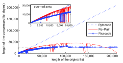
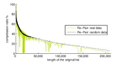
Re-Pair should exploit repetitions in the sets of documents where different words belong. It is well known that words do not distribute uniformly across documents [BYN04]. However, this is not the main source of the success of Re-Pair. To empirically validate this claim, we modified our inverted lists as follows: Each list of $\ell$ entries in $[1,u]$ was replaced by $\ell$ different random numbers in $[1,u]$. So the list lengths are maintained, but the skewness in the chosen documents is destroyed. Re-Pair compressed this new list to 64.24MB, compared to the 48.24MB obtained on the original list.

Figure 2 (right) shows the compression ratio achieved as a function of the length of the lists (dictionary excluded), for both the real and the random distributions. The behavior of Re-Pair is very similar in both cases, and thus it can be largely explained by combinatorial arguments and by the distribution of the list lengths. This is governed by Zipf Law [Zip49]. Nevertheless, simple binomial- and Poisson/exponential-based models that ignore interactions between consecutive pairs do not explain the results well; a more complex model should be used.

The real lists compress 25% more than the randomly generated ones. This is related to the parts of the plot where some words of intermediate frequency compress very well, and corresponds to positive correlation of word occurrences, that is, words that tend to appear in the same documents and thus generate the same pairs, which are thus easily compressed. Therefore, the uneven distribution of words across the collection [BYN04] is a non-negligible, yet secondary, source of Re-Pair compressibility, being Zipf Law the main one.

Finally, we have experimented with the maximum height of a rule to verify the hypothesis of logarithmic behavior. We packed 1 to 128 consecutive documents in the whole collection, so as to have an increasing number of (aggregated) documents. The growth of the maximum height is indeed logarithmic, starting from 15 when 128 documents are packed (fewest documents) and stabilizing around 25 when packing 8 documents. When we optimize the number of rules, the heights go to 9 and 19 respectively.

5.2 Time performance

We now consider intersection time. We show results for two different versions of the indexes. In the first scenario we assume that all the posting lists are compressed with Re-Pair, byte coding, or Rice codes. In the second scenario, we follow the ideas in [MC07] and represent the longest lists using bitmaps, and the remainder with the pure techniques.

5.2.1 Pure compression scenario: byte codes vs Re-Pair vs Rice

The outcome of the comparison significantly depends on the ratio of lengths between the two lists [ST07]. Thus we present results between randomly chosen pairs of words, as a function of this ratio. Due to its non-monotonicity, however, the results for Re-Pair depend on the absolute length of the lists. Thus we obtained results for different length ranges of the longer list. The results given in Figures 3 and 4 show times assuming that the longest list has around 100,000 values. We generated 1,000 pairs per plot and repeated each search 1,000 times; average times are computed grouping by ratio.

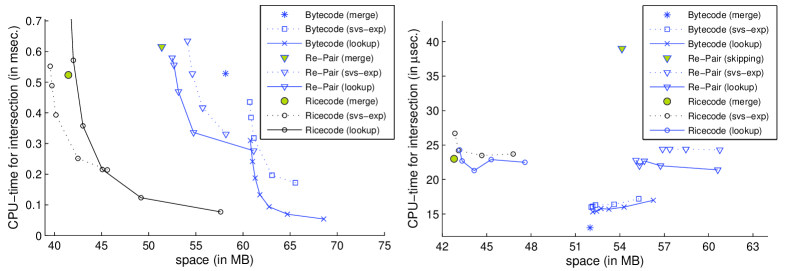
Figure 3 (left) shows some results. We chose variants using least space for byte codes (but they are still much larger than ours). The Rice variants used are clearly the least space demanding alternatives. When using merge, byte codes are faster than Re-Pair, yet the latter uses significantly less space.

Re-Pair with (b)-sampling and lookup search outperforms byte codes with (a)-sampling and exp search, even using less space (for $B=64$). Times only match if Re-Pair uses $B=256$, but then Re-Pair uses much less space than byte code-based ones. Also, Re-Pair with exp search is a bit slower than with lookup for about the same space. However, it still performs better than byte codes using exp  for the same space: Although not shown in the figure, Re-Pair with (a)-sampling and $k=1$ requires 58.18MB, whereas byte coding for $k=32$ needs 60.86MB, yet it performs similarly to Re-Pair with (b)-sampling and $B=64$, which requires only 54.75MB.

The results worsen a bit for Re-Pair on the shorter lists, as svs using exp search obtains similar results to Re-Pair with (b)-sampling and $B=64$, and merge becomes better than Re-Pair with no sampling. Again, (b)-sampling is the best choice for Re-Pair.

Our method dominates the time-space tradeoff when compared to byte codes with lookup, yet the latter allows to achieve better times by letting the structure use much more space than ours. The advantage of Re-Pair can be attributed to the fact that by achieving much better space, it allows to use a denser sampling, and to the ability of skipping phrases.

Rice coding behave particularly well in this scenario. They require much less space than the others (for example Rice with (a)-sampling and $k=4$ requires only 42.49MB), and even though when combined with either merge or lookup it is overcome by byte coding (but using much less space), it is very competitive when coupled with a svs intersection algorithm.

Figure 3: The intersection times as a function of the length ratios (the longest list has around 100,000 elements). Left: pure variants for Re-Pair and byte codes. Right: variants representing the longest lists with bitmaps following the approach in [MC07].

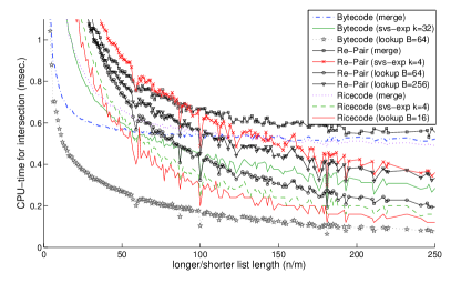
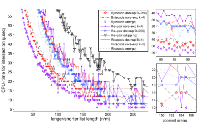
Figure 4 (left) shows this time-space tradeoff for those runs with $n/m$ values in the range $100\leq n/m\leq 200$. Our Re-Pair with no sampling achieves 13% better compression than byte codes with no sampling, hence we can use a denser sampling for the same space (and even less). The dictionary is negligible and it would fit in RAM for very large collections, even if it scaled linearly with the data. If we consider the dictionary and the resulting sequence, the total space is about 10% of the text size and, discounting vocabulary, about 25% of the plain integer representation of inverted lists. When packing 10 documents into one, Re-Pair total space improves even in relative terms: it is about 5% of the text, discounting vocabulary it is 20% of an integer inverted list representation, and it is 27% better than the byte code-based techniques.

Figure 4: Time-space tradeoff. Intersection times shown as the average of runs with $100\leq n/m\leq 200$. Left: pure variants for Re-Pair and byte codes. Right: variants representing the longest lists with bitmaps following the approach in [MC07].

5.2.2 Hybrid compression: bitmaps + pure techniques

In Figure 3 (right) we include the results representing the longest lists using bitmaps [MC07]. In this case the other methods outperform Re-Pair in almost all aspects. Figure 4 (right) shows the tradeoff offered by the three methods combined with the bitmap representation [MC07]. As mentioned above, the other structures improve further than ours with this approach, offering a better time/space tradeoff. On the one hand, by representing the longest lists with a bitmap, Re-Pair cannot benefit from the existence of the very repetitive gaps that occur on those lists (it was the main source of its good compression). On the other hand, byte coding has no longer to pay so much space for representing the longest lists. Note that the shortest codeword length is one byte for the byte codes.

Figure 5: Time-space tradeoff. Intersection times shown as the average of runs with $n\in\{10,50,100\}$ and, (left) $n\leq m\leq n\times 10$ or (right) $n\leq m\leq n\times 100$

.

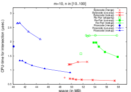
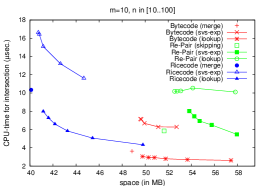
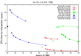
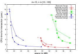
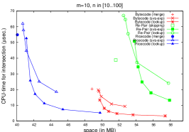
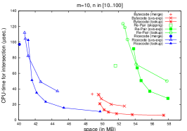
Figure 5 shows also values for different lengths of the shortest list $n\in\{10,50,100\}$ and the length of longest list $m$ such that $n\leq m\leq 10\textperiodcentered n$ (first row) and $n\leq m\leq 100\textperiodcentered n$ (second row) respectively. In these experiments, the maximum number of elements in the largest list (n) is always $n\leq 10,000$. As proposed in [MC07], we used the value $\frac{num\ of\ docs}{8}$ as a threshold for the number of elements a list must contain to be compressed with a bitmap. Therefore, we can ensure that no bitmap-compressed lists will be included in the intersection of two given lists. It can be seen that byte-coding is the fastest approach, Rice achieves the best compression values, and Re-Pair is clearly overcome in the space-time tradeoff. The comparison of merge with Rice codes against Re-Pair with skipping is more attractive for Re-Pair, as it takes again advantage of its implicit skipping features.

Given the results in both cases (with and without bitmaps), we conjecture that the loss of Re-Pair in the time/space tradeoff is due to the fact that Re-Pair does not gain as much compression as the other techniques when converting the longer lists to bitmaps. This suggests that the criteria for replacing a list and use a bitmap should be studied further. Our experiments expose a result that is of independent interest, namely the lookup strategy [ST07] with bitmaps achieves a better time/space tradeoff than the original proposal [MC07].

6 Conclusions

We have presented a novel method to compress inverted lists. While previous methods rely on variable-length encoding of differences, we use Re-Pair on the differences. The compression we achieve is not only much better than difference encoding using byte codes (which permits denser sampling for the same space), but it also contains implicit data that allows for fast skipping on the unsampled areas. Thus our method achieves a good time/space tradeoff in main memory which, as explained in the Introduction, is a scenario receiving much attention. When we include the technique proposed by Moffat and Culpepper [MC07], Re-Pair loses its advantage. Yet, we believe that further research in this line could achieve more competitive results for our Re-Pair representation. For example, we could represent with bitmaps the lists that remain long after compressing.

Because of its locality properties, we also expect our index to perform well on secondary memory. The vocabulary, the samplings, and the Re-Pair dictionary can realistically fit in RAM: all are small and can be controlled at will.

We have compared Re-Pair with difference encoding using byte codes, as they have been shown to offer a very good time/compression tradeoff [CM07]. Byte coding, however, is not the most space-efficient way to encode differences, as the experiments show in the results for Rice codes. This variant dominates the time/space tradeoff. In this aspect, it is interesting that there are also more compact representations of the Re-Pair output [CN08], which are potentially competitive on secondary memory.

Another interesting challenge is how to handle changes to the collection, where new documents are inserted into or deleted from the collection. The usual technique for insertions is to index the new documents and then merge the indexes, so that some symbols are appended at the end of several lists.

Finally, we also aim at compressed Re-Pair dictionary representations that allow descending faster in the parse tree, and at Re-Pair variants for compression of other types of inverted indexes, such as those used for relevance ranking.

Acknoledgements

This work was funded in part by NSERC of Canada and Go-Bell Scholarships Program (first author), by MEC grant TIN2006-15071-C03-03 (second author), by AECI grant A/8065/07 (second and third authors), and by Fondecyt grant 1-080019 (first and third authors).

References

- [AM06] V. Anh and A. Moffat. Pruned query evaluation using pre-computed impacts. In Proc. 29th SIGIR, pages 372–379, 2006.
- [BK02] J. Barbay and C. Kenyon. Adaptive intersection and t-threshold problems. In Proc. 13th SODA, pages 390–399, 2002.
- [BLOL06] J. Barbay, A. López-Ortiz, and T. Lu. Faster adaptive set intersections for text searching. In Proc. 5th WEA, pages 146–157, 2006.
- [BY04] R. Baeza-Yates. A fast set intersection algorithm for sorted sequences. In Proc. 15th CPM, LNCS 3109, pages 400–408, 2004.
- [BYMN02] R. Baeza-Yates, A. Moffat, and G. Navarro. Searching Large Text Collections, pages 195–244. Kluwer Academic, 2002.
- [BYN04] R. Baeza-Yates and G. Navarro. Modeling text databases. In Recent Advances in Applied Probability, pages 1–25. Springer, 2004.
- [BYR99] R. Baeza-Yates and B. Ribeiro. Modern Information Retrieval. Addison-Wesley, 1999.
- [BYS05] R. Baeza-Yates and A. Salinger. Experimental analysis of a fast intersection algorithm for sorted sequences. In Proc. 12th SPIRE, pages 13–24, 2005.
- [CM07] J. Culpepper and A. Moffat. Compact set representation for information retrieval. In Proc. 14th SPIRE, pages 137–148, 2007.
- [CN07] F. Claude and G. Navarro. A fast and compact Web graph representation. In Proc. 14th SPIRE, LNCS 4726, pages 105–116, 2007.
- [CN08] F. Claude and G. Navarro. Practical rank/select queries over arbitrary sequences. In Proc. 15th SPIRE, LNCS, 2008.
- [DM00] E. Demaine and I. Munro. Adaptive set intersections, unions, and differences. In Proc. 11th SODA, pages 743–752, 2000.
- [GN07] R. González and G. Navarro. Compressed text indexes with fast locate. In Proc. 18th CPM, LNCS 4580, pages 216–227, 2007.
- [Hea78] H. Heaps. Information Retrieval - Computational and Theoretical Aspects. Academic Press, 1978.
- [LM00] J. Larsson and A. Moffat. Off-line dictionary-based compression. Proc. IEEE, 88(11):1722–1732, 2000.
- [MC07] A. Moffat and S. Culppeper. Hybrid bitvector index compression. In Proc. 12th ADCS, pages 25–31, 2007.
- [Mun96] I. Munro. Tables. In Proc. 16th FSTTCS, LNCS 1180, pages 37–42, 1996.
- [NMN+00] G. Navarro, E. Moura, M. Neubert, N. Ziviani, and R. Baeza-Yates. Adding compression to block addressing inverted indexes. Inf. Retr., 3(1):49–77, 2000.
- [PZSD96] M. Persin, J. Zobel, and R. Sacks-Davis. Filtered document retrieval with frequency-sorted indexes. J. Amer. Soc. Inf. Sci., 47(10):749–764, 1996.
- [Sak05] H. Sakamoto. A fully linear-time approximation algorithm for grammar-based compression. Journal of Discrete Algorithms, 3:416–430, 2005.
- [SC07] T. Strohman and B. Croft. Efficient document retrieval in main memory. In Proc. 30th SIGIR, pages 175–182, 2007.
- [ST07] P. Sanders and F. Transier. Intersection in integer inverted indices. In Proc. 9th ALENEX, 2007.
- [Wan03] R. Wan. Browsing and Searching Compressed Documents. PhD thesis, Dept. of Computer Science and Software Engineering, Univ. Melbourne, 2003. http://eprints.unimelb.edu.au/archive/00000871.
- [WMB99] I. Witten, A. Moffat, and T. Bell. Managing Gigabytes. Morgan Kaufmann, 2nd edition, 1999.
- [Zip49] G. Zipf. Human Behaviour and the Principle of Least Effort. Addison-Wesley, 1949.
- [ZM06] J. Zobel and A. Moffat. Inverted files for text search engines. ACM Comp. Surv., 38(2):article 6, 2006.