A re–analysis of the iron line in the XMM-Newton data from the low/hard state in GX339–4

Abstract

The detection of an extremely broad iron line in XMM-Newton MOS data from the low/hard state of the black hole binary GX339-4 is the only piece of evidence which unambiguously conflicts with the otherwise extremely successful truncated disc interpretation of this state. However, it also conflicts with some aspect of observational data for all other alternative geometries of the low/hard state, including jet models, making it very difficult to understand. We reanalyse these data and show that they are strongly affected by pileup even with extensive centroid removal as the source is $\sim$ 200$\times$ brighter than the recommended maximum countrate. Instead, we extract the simultaneous PN timing mode data which should not be affected by pileup. These show a line which is significantly narrower than in the MOS data. Thus these data are easily consistent with a truncated disc, and indeed, strongly support such an interpretation.

1 Introduction

The current paradigm for the structure of the accretion flow in black hole binaries (hereafter BHB) at low luminosities is that the cool, optically thick, geometrically thin standard accretion disc is replaced in the inner regions by a hot, optically thin, geometrically thick flow (Esin et al. 1997). This model has gained widespread acceptance by its ability to provide a framework in which to interpret large amounts of apparently unrelated observational data by decreasing the truncation radius of the disc as the mass accretion rate increases. At the lowest luminosities, the lack of an inner disc means that there are few seed photons from the disc illuminating the flow, so the spectra are hard. Decreasing the disc truncation radius leads to greater overlap of the flow with the disc, so more seed photons to Compton cool the flow, giving softer spectra. This also gives a correlated increase in the amount of reflection and iron line produced by irradiation of the disc, and an increase in the broadening of these features by the stronger special and general relativistic effects. The decreasing radius also means that any frequencies set by this radius will increase, giving a qualitative (and sometimes quantitative) description of the increasing characteristic frequencies (including Quasi- Periodic Oscillations) seen in the power spectra and their tight correlation with the energy spectra. The flow is completely replaced by the disc when the disc reaches its minimum radius (last stable orbit), giving a physical mechanism for the marked hard-to-soft transition seen in black hole binaries. Even the jet behaviour can be tied into this picture, as a large scale height flow is probably required for jet formation, so the collapse of the inner flow as the disc reaches its minimum radius triggers a similar collapse of the radio emission (see e.g. the reviews by Remillard & McClintock 2006 and Done, Gierlinski & Kubota 2007, hereafter DGK07, with specific data on GX339-4 in e.g. Fender et al 1999; Belloni et al 2005).

Nonetheless, such models are ruled out despite these evident successes if the disc extends down to the last stable orbit in the low/hard state. There are two clear claims of this in the literature, first from a detection of an extremely broad iron line in the low/hard state of GX339-4 (Miller et al 2006 hereafter M06, Reis et al 2008 hereafter R08) and secondly from the detection of the residual thermal disc emission which is consistent with a disc extending down to the last stable orbit (M06; Rykoff et al 2007; R08, Reis, Miller & Fabian 2009). The direct disc emission can be alternatively interpreted as a truncated disc, especially when including the effects of irradiation of the inner disc (Cabanac et al 2009; Gierlinski, Done & Page 2008). There is also potential contamination by other components in soft X-rays, as must be the case in the well studied dim low/hard state spectra from XTE J1118+480. This system has very low absorption, allowing the cool, truncated disc emission to be seen in the UV/EUV (Esin et al 2001) while the soft X-ray excess is clearly hotter and less luminous (Reis, et al 2009; Chiang et al 2009; perhaps arising from the jet: Brocksopp et al 2010).

Thus the extreme broad iron line in the XMM-Newton data of GX339-4 is the only strong evidence against the truncated disc/hot flow models for the low/hard state (Tomsick 2008). If this is a unique interpretation of the data then it is sufficient evidence to rule out the hot inner flow/truncated disc geometry and to require an alternative picture for the low/hard state. However, there are strong constraints on the geometry of any cool disc with respect to the hard X–ray source which arise from reprocessing. We outline these, and show that the extremely broad line conflicts with some aspect of the observational data for all current alternative geometries for the low/hard state, even that of a mildly relativistic beaming of the hard X-ray associated with jet model (Beloborodov 1999).

These conflicts motivate us to re-examine these data from the low/hard state of GX 339-4 to see how robust the iron line parameters are. We find that while the description of the line in the data is robust, the data themselves are not. The source is $\sim 200\times$ brighter than the recommended limit for pile up in the data modes used. We show that pileup is still an issue even excluding the central 18” core of the image and using only single events as in M06. R08 reanalysed these data excluding a 50” core, using single plus double events. We show that while the singles are probably free from pileup at this large radius, the doubles are not, so these data are still affected, plus there are additional uncertainties form response and background.

Instead, we extract the PN data which is in timing mode so is not strongly affected by pile up. These give a line which is clearly narrower than that of M06 and R08. This narrower line is also consistent with the simultaneous RXTE data, contrasting with the extreme broad line from the MOS data which requires the addition of an ’instrumental’ edge feature at 4.78 keV in RXTE. We fit both simple and sophisticated models to the PN spectrum, and show that the line in these data strongly supports a truncated disc interpretation of the low/hard state. This conclusion is further strengthened by Suzaku data from a lower luminosity low/hard state of GX339-4 which also show a narrow line (Tomsick et al 2009).

2 Potential alternative geometries for the low/hard state

The main problem is to explain how an extremely broad line can co-exist with a hard spectrum. The line is produced by X-ray illumination of the disc and the fraction of emission which is not reflected is (quasi)thermalised, adding to any intrinsic soft flux from the disc. Some fraction of this flux is re-intercepted by the corona, increasing its Compton cooling, and making the spectrum softer. It is this coupling between the reflected emission and the corona seed photons via reprocessing which makes it difficult to maintain a hard spectrum from the corona in the presence of a cool material which extends down close to the black hole.

For example, if the corona extends smoothly over the disc in a sandwich geometry then all the reprocessed photons are re-intercepted by the corona. If the reprocessed emission thermalises, then it adds to the soft photons for Compton cooling. Energy balance then gives spectra which are necessarily steep, in conflict with the observed hard spectra which define the low/hard state (Haardt & Maraschi 1993). Compton anisotropy in this plane parallel geometry can harden the observed spectrum in the first few scattering orders (Haardt & Maraschi 1993), but this then predicts a break at higher energies which is not seen in the data (Barrio, Done & Nayakshin 2003). Alternatively, extreme ionisation of the disc could prevent thermalisation of the reprocessed flux, but this requires some very specific conditions which may not be physical (constant density disc atmosphere rather than hydrostatic equilibrium: Malzac et al 2005).

Another way to make a hard spectrum with a corona above the disc is if the corona is patchy rather than smooth, or forms a ’lamppost’ above the spin axis. In either geometry, a large fraction of the reprocessed flux need not re-intercept the corona and cool it, so can produce hard spectra (Stern et al 1995; Malzac et al 2005), while the illumination of the disc gives the line. However, this illumination should also give rise to an accompanying continuum reflection signature, and these reflected photons are then likewise not re-intercepted, predicting a strong reflection signature to accompany a strong, broad line. Yet the observed amount of reflected continuum (and line) is generally rather weak in the low/hard state (around $\sim 0.3\times$ that which would be expected if the disc covered half the sky as seen from the X-ray source for these GX339-4 data: see Fig 10 of R08), but both line and amount of reflection increase together as the spectrum softens (e.g. Gilfanov, Churazov & Revnivtsev 1999; Ibragimov et al 2005; DGK07). This can be due to a changing illuminating geometry or a changing ionisation state (see below). The changing geometry has an obvious origin in the truncated disc model, with increased reflection (and smearing) as the disc extends further into the hot flow, correlated with a steeper spectral index as more seed photons illuminate the Comptonising region. Instead, if the disc inner radius is fixed, then the source geometry has to change. In a patchy corona this can be linked to its covering fraction over the disc, but this gives the opposite trend to that seen in the data. A higher covering fraction of the corona over the disc gives steeper spectra by intercepting more (reprocessed and intrinsic) flux from the disc but also means that less of the reflected emission can escape (Malzac et al 2005). Conversely, in a static ’lamppost’ model there is no possible geometry change.

Nonetheless, even without a changing geometry, the contrast of the reflection features with respect to the illuminating continuum can change with ionisation state of the material. Extreme ionisation effects can lead to a suppression of the apparent amount of reflection below 20 keV as this removes the characteristic atomic features. Thus the change in amount of reflection discussed above could instead be a result of changing ionisation rather than geometry. However, ionisation has no effect on the high energy shape of the reflected emission as this is determined only by Compton downscattering losses. Thus the shape of the high energy spectrum (50-200 keV) constrains the total amount of reflection, and this clearly shows that the amount of reflection in the low/hard state is intrinsically low (Maccarone & Coppi 2002; Barrio, Done & Nayakshin 2003).

The combination of observed small solid angle of reflection with a hard spectrum (i.e. small inferred seed photon flux from reprocessing) can be reconciled with an underlying disc only if the hard X-rays are anisotropic. An attractive origin for this is the mildly relativistic jet seen in the low/hard state, with resultant mild beaming of the X-ray irradiation away from the disc (Beloborodov 1999, Ferreira et al 2006). These models, with a cool, passive disc down to the last stable orbit acting as an anchor for the magnetic fields which launch the jet, then seem to give a possible origin for the broad iron line. However, the broad line itself is inconsistent with this geometry as it requires an emissivity which is strongly centrally peaked (M06; R08). This is opposite to the less centrally concentrated beaming pattern which arises from a mildly relativistic jet. Instead, such centrally concentrated emission could be produced either by strong lightbending for a source very close to the black hole (Miniutti et al 2003; Miniutti & Fabian 2004), or by the X-ray source moving towards the disc e.g. a failed jet (Henri & Petrucci 1997; Ghisellini et al 2004). However, both of these then lead to enhanced reflection fractions, rather than the small reflection fractions observed. The alternative jet models of Markoff, Nowak & Wilms (2005) also converge on the truncated disc, hot inner flow geometry, so do not offer a way to produce the broad line.

Instead, perhaps the combination of scarcity of seed photons to give the hard spectrum and a (very centrally concentrated) broad iron line could be reconciled if the cool reflecting material were not a complete disc, but formed only a small ring close to the innermost stable orbit. In effect this is a reversal of the truncated disc/hot flow model, with the disc on the inside, and the hot flow on the outside. Such a geometry may form close to the major hard-soft spectral transition from disc evaporation/condensation (Liu et al 2007). While this is a potentially viable model (see also Chiang et al 2009), it runs into subtle problems with the very rapid spectral variability. The fastest variability has harder spectrum (and less reflection) than the slower variability (Revnivtsev, Gilfanov & Churazov 1999), leading to a complex series of time lags across the spectrum (Miyamoto & Kitamoto 1989; Poutanen & Fabian 1999). This can be explained in the standard truncated disc/hot inner flow models as the larger timescale variability is characteristic of the larger radii regions of the hot flow. This is the region of overlap between the hot flow and truncated disc, so giving more seed photons and reflection. Conversely, the most rapid variability is produced in the innermost regions, where there is no overlap with the disc and the spectra are harder (Kotov et al 2001; Arevelo & Uttley 2006). The inner ring of material reverses this, predicting that the fastest variability has the softest spectra and most reflection, contrary to the observations.

Thus while there is an obvious conflict between an extremely relativistically broadened line and the truncated disc models, all other alternative geometries currently suggested for the low/hard state also have issues with this observation. Assuming that the line shape is robust, and is set by relativistic effects alone (with no contribution from scattering in an outflow: Titarchuck et al 2009; Sim et al 2010), then there appears to be no geometry which can simultaneously explain the line shape together with a hard continuum spectrum in these data without giving rise to potentially serious problems with other observations.

3 XMM-Newton Data Selection and Extraction

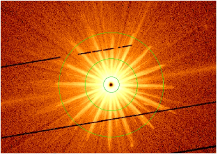
Figure 1: MOS1 image, with the black centre showing the extreme pileup. The circles have radii 18, 60 and 120 arcsec from the center. We extract spectra from single events only from 0-120, 18-120, 60-120 and (not shown) 90-120 arcsecond regions.

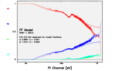
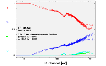
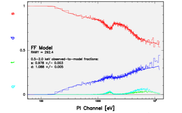
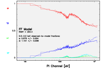
Figure 2: Quantative measures of pileup in the MOS1 camera using the SAS task epatplot. The data points show the fraction of events which register as singles (s), doubles (d), triples (t) and quadruples (q), while the line shows the expected fraction for non-piled up data. The upper panels show the data extracted from 0-120 and 18-120 arcsec regions, while the lower panels show 60-120 and 90-120 arcseconds. The deviations between the expected and observed pattern distributions are clearly present even for the singles for the 0-120 arcsec data above 3 keV, and for 18-120 above 6 keV. The 60-180 and 90-120 singles distribution appears clean, though the doubles probably are still affected above 7 keV.

The XMM-Newton Observatory (Jansen et al 2001) includes three 1500 cm² X-ray telescopes each with an EPIC (0.1–15 keV) at the focus. Two of the EPIC imaging spectrometers use MOS CCDs (Turner et al 2001) and one uses PN CCDs (Struder et al 2001).

We analysed XMM-Newton observations 0204730201 and 0204730301, taken in revolutions 782 and 783, starting at 2004-03-16 16:23:41 and 2004-03-18 17:19:49, respectively. The MOS data are taken in Full Frame mode, with the medium filter in place, while the PN data are in timing mode, again with the medium filter. Data products were reduced using the Science Analysis Software (SAS) version 9.0 (beta). This includes an update in calculating the ancillary response files for non-contiguous extraction regions for timing data, as required for excluding the central columns to check for pileup.

The events list were screened against times with high instrumental flaring. This resulted in net exposures time of 66, 81 and 81 ks for EPIC pn, MOS1 and MOS2 cameras for observation 0204730201 and of 53, 70 and 70 ks for EPIC pn, MOS1 and MOS2 cameras for observation 0204730301.

The source was very bright, and the PN data (see below) give a 0.4-10 keV flux of $1.3\times 10^{-9}$ ergs cm^-2 s^-1 for a single power law fit with $\Gamma=1.55$ and $N_{h}=4.1\times 10^{21}$ cm^-2. This gives a WebPIMMS predicted count rate for the MOS in full frame mode with the medium filter of 61 c/s for a 15” extraction region, or total of $\sim 120$ c/s, nearly 200$\times$ larger than the 0.7 c/s recommended total count rate limit for pileup not to affect the spectra. Instead, the measured count rate for a 15” extraction region is 4.4 c/s, as the central part of the image is so badly piled up as to be black (see Fig.1).

’Photon pile-up’ occurs when a source is so bright that there is the non-negligible possibility that two or more X-ray photons deposit charge packets in a single pixel during one read-out cycle (i.e. one frame). This leads to complete flux loss in the central part of the source if the summed energy of the two photons is larger than the reconstructed energy rejection threshold, or spectral hardening if the summed energy is below the rejection threshold. In addition, pattern pile-up occurs when two or more X-ray photons deposit charge packets in neighbouring pixels within the same frame e.g. two single soft events will be interpreted as a double event with twice the energy. Again, this leads to flux loss or spectral hardening depending on whether the summed energy of the event is above or below the rejection threshold.

3.1 MOS data

The EPIC MOS Full Frame Mode reads out all pixels of all CCDs, covering the full field of view. We first extract a source spectrum from a 120 arcsec radius circle centred on the source position (largest circle in Fig. 1) and illustrate the extent of pileup on these using the SAS task epatplot. Fig.2a shows the distribution of observed single- and double- pixel (and more complex) events together with their expected values. The effects of pile-up are evident when the data and model distributions diverge, as is clearly the case here above 4 keV. The effects of pile-up will be different for each source, depending on the spectral shape (see XMM-Newton Users Handbook for some examples).

Pileup cannot yet be corrected, but its effects can be mitigated in imaging modes by excising the heavily piled-up core from the image, and extracting counts in an annulus which includes only the lower count rate wings of the point spread function (see XMM-Newton Users Handbook). We follow M06 and exclude the inner 18” region (smallest circle in Fig. 1). M06 chose this radial range by using epatplot to assess the extent of pileup. We show the epatplot results in Fig. 2b. There is still a marked deviation in the distribution of observed events from the expected curve above 6 keV (somewhat better than the 4 keV for the full data, but still clearly affected by pileup).

epatplot also integrates the observed ratios over a given energy range to quantify the amount of pileup. The default range is 0.5-2 keV as this is most sensitive to pileup for soft photon spectra. The observed distribution of single events in this bandpass is within $\sim 3\sigma$ of the expected value (M06). However, the spectrum of GX339-4 is very hard, so the effects of pileup are instead most noticeable at high energies so this default bandpass is not very sensitive to the extent of pileup. These ratios are clearly incompatible with unity in the 6-10 keV band. Pileup strongly affects the spectrum above $\sim$ 6 keV even excluding the central 18 arcmin and extracting only single events.

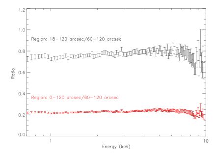
Figure 3: A model independent way to show the effect of pileup on the spectra. The ancillary response file (arf) for each spectrum is used to correct the counts in each channel for the effective area. We ratio these corrected counts for 0-120s/60-120s and 18-120s/60-120s. If pileup were not important, these ratios should be unity at all energies. This is plainly not the case. The 0-120s/60-120s shows that many counts are lost from the 0-120s spectrum due to pileup, and that this is not a constant factor but depends on energy. While many fewer counts are lost from the 18-120s spectrum, the energy dependence is clearly not flat but results in a broad curvature of the spectrum with obvious implications for modelling the red wing of the iron line.

We exclude progressively larger central regions and find that we need to go beyond 60 arcsec before the ratio of observed to expected fraction in epatplot is consistent (at $3\sigma$) with unity in the 6-10 keV for the single events. The distribution for the doubles still appears inconsistent, but the much poorer statistics means that this is not significantly different from unity. Thus the spectra extracted by R08 (singles, doubles and quadruple events, excluding a 50 arcsec core) should be mainly free from pileup in singles alone, but doubles and quadruples could still be affected.

This is at first sight surprising as the count rate per pixel is nominally below the recommended on axis surface brightness limit of $4.9\times 10^{-4}$ c/s/arcsec² (i.e. 0.35 c/s in a 15” radius circle). This shows that the effects of pileup can be subtle, and in fact the double events still deviate from the expected curve above 6 keV even for data extracted from 90-120”, though again the statistics are so poor that this is not significantly different from unity (see Fig. 2d).

We use the spectrum extracted from single events in a 60-120 arcsec annular region (hereafter 60-120s) as our reference spectrum to try to assess the effect of pileup in the spectra extracted from singles in the 18-120 arcsec region (hereafter 18-120s) and singles extracted in the 0-120 arcsec region (hereafter 0-120s). We generate ancillary response files (arf’s) using the SAS task arfgen for the three spectral regions, and for each spectrum we divide each energy channel count rate by its effective area at that energy as given by the arf. This corrects for the differing effective areas in each extraction region, so we can take a ratio of the spectra to show the effect of pileup in a model independent manner. Fig. 3 shows this for 0-120s (lower, red) and the 18-120s data (upper, black). These ratios should be unity if the arf generation is correct and no counts are lost in pileup. Instead, the full region gives a mean value of 0.2, suggesting that the intrinsic count rate was close to $\sim 120$ counts/sec, as predicted! More importantly, the ratio is not flat, showing the derived spectra are distorted. This curvature is not large but is very significant as the error bars are small. Conversely, the 18-120s data are much closer to the expected normalisation, showing that many fewer counts are lost, but there is now clear curvature from the deficit of high energy single events noted by epatplot above 6 keV. This results in a broad residual which could clearly affect the determination of the iron line width.

We test this explicitly by fitting the spectra directly. While background is negligible for the 18-120s spectrum, it is much more important for the 60-120s spectrum. We follow M06 and R08 and extract background from a 60 arcsec region towards the corner of the chip. We fit this in the same way as M06, i.e. with an absorbed (tbabs) multicolour disc (diskbb) plus power law to describe the continuum over 0.7-10 keV, excluding the 4-7 keV iron line bandpass. Fig.  4 (red points) shows the ratio of the model to the data over the full bandpass, with a strongly skewed line residual as in M06. The blue points shows the 60-120” data ratio to the same continuum model. The residuals in the 4-7 keV region are quite different, with no apparent line detected, but with a strong drop above 7 keV.

The decrease in strength of the red wing, and increasing strength of the drop above 7 keV is also shown by R08 for progressively larger extraction regions. These data show that for a continuum model set by the 18-120s spectrum, the red wing progressively disappears and the 7-10 keV continuum drops. This is a clear sign of pileup in the spectra with small extraction regions, as confirmed by the epatplot results (Fig.2b). However, allowing the model to float between the different datasets gives a steeper underlying continuua spectra for the larger extraction regions, which recovers the broad wing (Fig 1b in R08). This constant residual profile was used by R08 to argue that the 18-120s spectrum as in M06 was not affected by pileup.

However, this line profile in the 60-120s data is strongly dependent on the background used. The corners of the chip are furthest from the source position, but the source is so bright that the point spread function puts significant counts into these regions. This is seen both from comparing the putative background (chip corner) count rate with that seen at larger off axis angles from the other MOS1 chips and by comparing to another observation of GX339-4 where the source was ultrafaint (0085680501). Both these give a significantly lower countrate, showing that the the chip corners are contaminated by the source. Photons scattered into the far wings of the PSF are harder than average, so this results in the background being contaminated by a harder version of the source spectrum. Background subtracting with these data then artificially steepens the derived source spectrum at high energies, which in turn leads to a broad residual in the 4-7 keV from fits which exclude this energy band.

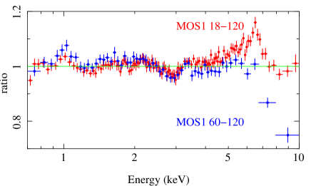
Figure 4: Ratio of the MOS1 18-120s spectrum as in M06 (red) to the best fit continuum model excluding the 4-7 keV region. The blue points show the 60-120s data ratio’d to the same model. The 18-120s spectrum has more counts at high energies, as expected from pileup (see Fig. 2b), but it also has a much stronger ’red wing’. The 60-120s data have almost no line emission, but instead are dominated by a strong drop at 7 keV (see also R08).

In summary, the MOS data extracted from 18-120 arcsec are clearly piled up, even in single events. Extraction regions of $\sim$ 60 arcsec are required before the single event spectra are usable, though the double (and higher) events still show signs of pileup. Such large exclusion regions means that the statistics are poor, leading to increased systematic uncertainties from background (and response) issues. This combination of factors mean the MOS data and background are effectively unusable as shown.

3.2 PN data

3.2.1 Data Selection

The PN are in timing mode where only one CCD chip is operated. The data are collapsed into a one-dimensional row (4$\aas@@fstack{\prime}$4) and read out at high speed, with the second spatial dimension being replaced by timing information. This allows a time resolution of 30 $\mu$s, and photon pile-up occurs only for count rates $\mathrel{\hbox{\hbox to0.0pt{\hbox{\lower 4.0pt\hbox{$\sim$}}\hss}{\raise 2.0pt\hbox{$>$}}}}$800 counts/s. Before examining the pile-up effects with the epatplot output, we used the SAS task epfast on the EPIC pn event files to correct for a Charge Transfer Inefficiency (CTI) effect which has been seen in EPIC pn Timing mode when high count rates are present .

WebPIMMS gives an estimated total count rate of 260 c/s for the PN medium filter in timing mode for pattern 0 events. This is lower than the 800 c/s limit of this mode, but the source is hard so there is the possibility of print through of X-ray photons during the offset map calculation, which effectively reduces this limit by a factor of 2 (see Section 3.3.2 of the XMM-Newton users handbook). However, the source is very variable so it can exceed this limit. This variability can also cause the telemetry limit to be exceeded (at $\approx 450$ c/s for this mode if both MOS cameras are operated), at which point the science data are lost. Thus the telemetry limit is actually the more stringent constraint, and effectively excludes the most pileup data (see Section 3.3.2 of the XMM-Newton handbook), though short time periods of higher count rate can be registered before the buffer fills.

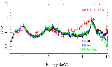
Figure 5: Ratio of PNall (black) to its best fit continuum model, excluding the 4-7 keV region. The blue and green points show the same model ratio’d to the PN3col and PN3colbgd spectra. All these PN spectra are very similar except at the highest energies, where PN3colbgd (green) is steeper than PN3col (blue), which is steeper than PNall (black). We also show the MOS1 18-120s spectrum ratio’d to its own best fit continuum model as in Fig. 4. The line profile is significantly broader in the piled up MOS data than in any of the PN spectra.

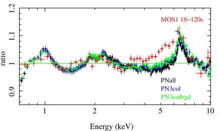
Figure 6: As in Fig. 5 except that all PN spectra are fit with their own best fit continuum models. The difference at high energies is therefore supressed by the power law becoming progressively steeper from PNall (1.53) to PN3col (1.56) to PN3colbgd (1.59). This results in progressively broader line residuals, but none are as broad as seen in the (pileup) MOS spectrum 18-120s.

First we extract a spectrum from columns 31–45. While single events should be less affected by pileup, there is a difficulty in uniquely registering such events in timing mode as these include photons which hit two adjacent pixels (i.e. doubles) separated in the readout direction. Hence we extract single+double events and refer to this as PNall. We fit these data to the simple absorbed disc plus power law model for the continuum, excluding the 4-7 keV region. The ratio of the data to this fit is shown in as the black points in Fig 5. The red points show the corresponding ratio for the 18-120s MOS spectrum (to its own best fit continuum model). The difference in the line shape is immediately apparent.

However, Fig 5 also shows that there are other residuals at energies of $\sim$ 1.0, 1.8 and 2.2 keV. The $\sim 1$ keV feature is often seen in other LMXRBs though its exact nature is still unclear (e.g. Sidoli et al 2001, Boirin & Parmar 2003; Boirin et al 2004; 2005; Diaz Trigo et al 2006; 2009). The features at 1.8-2.2 keV probably are artifacts of incomplete CTI correction in the PN timing mode.

We check for pileup in the PN data using epatplot. This shows small deviations between the observed and predicted ’single’ and double event ratios for PNall, with larger features around the instrument edges at 0.5 keV, 1.8 keV and 2.2 keV. Thus these are most probably associated with incomplete CTI correction. However, the number of singles is systematically below the predicted curve at all energies, while the doubles are systematically above. This could be indicative of pileup, but the constant ratio of the effect at all energies appears more likely to indicate a systematic error in modelling the number of singles and doubles in this mode (which is complicated as the exact pattern distribution depends on the asymmetrical shape of the charge cloud, and the projection of this on the readout direction: Kendziorra et al 2004).

We can check this by intensity slicing the PNall data, accumulating spectra from 0-200, 200-400, 400-600 and $\geq 600$ c/s. If pileup is important then this will progressively harden the brighter spectra. However, simple disc plus power law fits indicate that the spectrum is systematically softer for brighter spectra ($\Gamma=1.54$ compared to $\Gamma=1.62$ for the dimmest and brightest spectra, respectively). This shows that the intrinsic spectral variability (steeper when brighter, as in generally seen in the low/hard state e.g. Churazov et al 1999; DGK07) is more important than any residual pileup in these data.

Nontheless, we also re–extracted the data excluding the central 3 columns of the data in a technique analogous to excluding the central region of imaging data (PN3col). The epatplot results again have features at the instrument edges, but now the difference at other energies is much smaller. The blue points in Fig. 5 shows the ratio of these data to the same best fit continuum model as used for the PNall data. They are extremely similar except at the highest energies, where PN3col is steeper than PNall. This difference cannot be due to background as this would be more important for the lower count rate PN3col spectrum, and would effectively harden rather than soften its high energy spectrum.

It is possible then that pileup is causing the slight softening of the PN3col spectrum compared to PNall. However, it is also possible that this simply represents the limit on our current knowledge of the reconstructed pattern distribution and energy dependence of the point spread function in this mode. Hence we use both these spectra to illustrate the range of models allowed by the data.

Figure 7: The upper panel shows the PN timing mode lightcurve of the dipping source XB1254-690 extracted from columns 30-44, while the lower panel shows that from ’background’ channels 10-18. It is clear that a source of this brightness (around 250 c/s) contaminates the chip even at large off axis angles.

For the PN3col data, the lower count rate means background may become important. However, there are no source-free background regions on the PN chip as the source contaminates the background event even in the lowest/highest chip columns. This background contamination is worse than in the MOS cameras due to the smaller field of view ($13.6\times 4.4$ arcmin in the PN versus $10.9\times 10.9$ arcmin for the MOS, but the collapsed column for PN timing mode is the larger one, so the maximum angle for background extraction is 2 arcmin compared to 5 arcmin for the MOS). The amount of background contamination is more easily seen in the PN timing data from XB 1254-690. This is a dipper, so the source drops dramatically in intensity (e.g. Diaz Trigo et al 2006). Fig. 7 shows the source lightcurve together with the ’background’ lightcurve taken from columns 10-18 (as used by Wilkinson & Uttley 2009, hereafter WU09). The background shows the same dip structure as the source, showing that it is dominated by source photons scattered out into the far wings of the PSF. Again, since the PSF is energy dependent, these scattered photons are harder than the real source spectrum so this source contaminated background spectrum is not equivalent to subtracting a small fraction of the source spectrum plus background. Restricting the background to columns 3-14 reduces the effect slightly (the source counts increase from 95.8 per cent to 96.8 per cent), but the lightcurve of these columns from XB 1254-690 still shows that they are contaminated. A better estimate of the true background level can be made by extracting timing data from the observation in which GX339-4 was so faint as to be undetectable (0085680501). Using these data as background increase the source contribution to 99.8 per cent, showing that neglecting background in the PN3col spectrum is more appropriate. Nontheless, we also include a background subtracted PN3col spectrum (hereafter called PN3colbgd), using background from columns 10-18 in order to compare directly with the results of WU09).

We add 2 per cent systematics to account for uncertainties in the response, though since the data are grouped by a factor 4 then this results in a 1 per cent systematic error on the final spectrum and fit the data in the 0.7-10 keV range.

3.2.2 Iron line profile

model	$R_{in}$	$\beta$, inc	$kT_{disk}$	$N_{disk}$	$\Gamma$	$N_{pl}$	$E_{line},\xi$	$N_{line},N_{ref}$	$\chi^{2}/\nu$
	$R_{g}$		keV				keV	$\times 10^{-3},\times 10^{-5}$
				PNall
laor	$177_{-70}^{+3}$	$3$, $60^{\circ}$	$0.29(1)$	$1920_{-380}^{+530}$	$1.52(1)$	$0.186(2)$	$6.63_{-0.02}^{+0.03}$	$0.60(4)$	$938/221$
	$25_{-6}^{+1}$	$10_{-3.3}^{peg}$, $16\pm 1$	$0.29(1)$	$2100_{-550}^{+390}$	$1.53(1)$	$0.187(2)$	$6.95\pm 0.03$	$0.64(4)$	$925/219$
reflionx	$170\pm 70$	$3$, $60^{\circ}$	$0.33(1)$	$790_{-20}^{+110}$	$1.53(1)$	$0.178(1)$	$370_{-20}^{+10}$	$0.56(2)$	$502/220$
	$25_{-6}^{+7}$	$3$, $27(3)$	$0.34(2)$	$630_{-170}^{+170}$	$1.53(1)$	$0.176(2)$	$490_{-40}^{+10}$	$0.44(4)$	$468/219$
				PN3col
laor	$19\pm 4$	$3$, $60^{\circ}$	$0.26(1)$	$3890_{-930}^{+1000}$	$1.57(1)$	$0.198(2)$	$6.4_{peg}^{+0.03}$	$1.34(12)$	$762/221$
	$8.2_{-1.0}^{+1.2}$	$3.4(2)$, $17_{-2}^{+3}$	$0.26(1)$	$4400_{-960}^{+1479}$	$1.57(1)$	$0.198(2)$	$7_{-0.02}^{peg}$	$1.11(10)$	$716/219$
reflionx	$100_{-40}^{+60}$	$3$, $60^{\circ}$	$0.26(2)$	$3070_{-1150}^{+940}$	$1.58(2)$	$0.188(2)$	$260_{-20}^{+40}$	$1.16(28)$	$488/220$
	$11_{-3}^{+2}$	$3$, $25(3)$	$0.30(2)$	$1060_{-350}^{+650}$	$1.56(1)$	$0.182(3)$	$500_{-60}^{+20}$	$0.54(10)$	$396/219$
				PN3colbgd
laor	$24_{-4}^{+1}$	$3$, $60^{\circ}$	$0.23(1)$	$8560_{-1950}^{+2520}$	$1.60(1)$	$0.200(3)$	$6.4^{+0.01}$	$1.33(9)$	$667/221$
	$6.33_{-0.08}^{+1.04}$	$3.4(2)$, $22_{-3}^{+1}$	$0.23(1)$	$7960_{-1960}^{+3300}$	$1.60(1)$	$0.200(3)$	$7_{-0.02}^{peg}$	$1.43(12)$	$614/219$
reflionx	$60^{+40}_{-20}$	$3$, $60^{\circ}$	$0.22(1)$	$8000_{-2500}^{+4400}$	$1.61(1)$	$0.189(2)$	$250^{+10}_{-10}$	$1.19(26)$	$456/220$
	$10_{-2}^{+2}$	$3$ $27(3)$	$0.24(2)$	$4240_{-1820}^{+3210}$	$1.59(1)$	$0.179(3)$	$530_{-30}^{+30}$	$0.46(6)$	$360/219$
				MOS 18-120s
laor	$47\pm 15$	$3$, $60^{\circ}$	$0.29(2)$	$2790_{-800}^{+1100}$	$1.55(2)$	$0.198(4)$	$6.4^{+0.01}_{peg}$	$1.06(20)$	$309/218$
	$2.6_{-0.6}^{+0.3}$	$3.2(2)$, $0^{+30}_{peg}$	$0.31(2)$	$1770_{-370}^{+1030}$	$1.57(2)$	$0.200(5)$	$6.95_{-0.25}^{+0.05}$	$3.27(27)$	$220/216$
reflionx	$44_{-20}^{+20}$	$3$, $60^{\circ}$	$0.27(2)$	$3850_{-1380}^{+1650}$	$1.61(2)$	$0.211(7)$	$10_{peg}^{+3}$	$53(20)$	$297/217$
	$2.0_{-0.77peg}^{+0.6}$	$3$, $21(6)$	$0.32(1)$	$1400_{-400}^{+400}$	$1.56(2)$	$0.172(10)$	$500_{-180}^{+80}$	$1.07(13)$	$200/216$

Table 1: The various PN spectra fit with a simple diskbb+po+laor model (first two lines) and a more physical diskbb+po+kdblur*reflionx+gau model (second two lines). For each model the emissivity and inclination are first fixed at $3$ and $60^{\circ}$, respectively. Both these parameters are then allowed to be free for the laor model, but the resulting emissivity generally close to $3$ so this is fixed in the more complex reflection fits when the inclination is a free parameter. The corresponding column density is $0.42-0.44$, $0.45-0.48$, $0.48-0.51$ and $0.49-0.54\times 10^{22}$ cm^-2 for each of the 4 spectra. A narrow (width fixed at 0.01 keV) gaussian line at 6.4 keV is also included in the reflection fit, as there is a significant residual here, although its equivalent width is small.

We redo the Fig 5, but this time ratio each PN spectrum with its own best fitting model, where only the absorption is tied across the three datasets. The differences in the PN spectra at high energies means that this gives a progressively steeper power law spectra for PNall, PN3col and PN3colbgd, (1.53, 1.56 1.59 respectively). This results in progressively slightly broader line residuals for the 4.0-7.0 keV region excluded from the continuum fit as shown in Fig. 6. However, these are all still obviously narrower than the line from the MOS 18-120s data.

We quantify the differences in line profile between the MOS and PN by fitting each spectrum separately with a model of tbabs*(diskbb+po+laor), where the intrinsic line energy is constrained to be between $6.4-7.0$ keV. We first fix the inclination at $60^{\circ}$ (a reasonable value for the binary inclination in GX339-4: Kolehmainan & Done 2010) and the laor line emissivity at $3$. Then we allow both inclination and emissivity to be free parameters for each spectrum. All the PN spectra show a better fit for a solution with much lower inclination as the line profile in the PN data is quite symmetric rather than being skewed to the red. The smaller Doppler shifts from a lower inclination then require a smaller radius to get the same line width, but all of the PN data are consistent with a disc which does not extend below $6R_{g}$. By contrast, the piled up MOS 18-120s spectrum strongly requires a much smaller inner radius.

To have confidence in the line parameters requires modeling the reflected continuum as well as the line. We use the reflionx model for an ionised slab of constant density (Ross & Fabian 2005). This includes Compton scattering within the disc itself which can be important at high ionisation (Ross, Fabian & Young 1999), making the line intrinsically broad. We convolve this with relativistic effects using kdblur (based on the laor line kernel) model, and also include a narrow, neutral iron line, as this is plainly present as a small residual. Again we first fix the inclination and emissivity at $60^{\circ}$ and $3$, respectively. We then allow the inclination to be free, but keep the emissivity fixed at $3$ since the laor models showed that this is generally close to the derived value. We checked that there is no significantly better fit produced by allowing this to be free. Full details of all the parameters for these fits are given in Table 1.

Unsurprisingly, the full reflection model always gives a substantially better fit than the equivalent laor line fits. The data still prefer a lower inclination solution ($\sim 30^{\circ}$) than seems likely from the binary orbit (Kohlemainen & Done 2010), but we caution that this depends on the model used for both the continuum and reflected emission (the continuum is unlikely to be a single power law: see e.g. DGK07 section 4.3, and the detailed shape of the reflected spectrum depends on the assumed vertical structure of the disc: Malzac et al 2005). We will explore this further in a subsequent paper. Here we only concentrate on the iron line, and it is clear that the fits do not require an extreme relativistic profile for any of the PN spectra, with the inner disc always being larger than $6R_{g}$ even for the low inclination solutions, while the physically more likely higher inclination solutions strongly require a truncated disc.

The normalisation of the disc component is also a tracer of the inner radius of the accretion disc. This is consistent with a constant at $\sim 4700$ in the disc dominated high/soft state of GX339-4 (Kohelmainen & Done 2010; DGK07 fig. 13b). M06 claim that the disc component seen in the MOS 18-120s spectrum is consistent with the same inner radius, arguing against disc truncation. However, at face value, the disc normalisations for both MOS and PN are substantially lower (see also DGK07 fig 13b), except for the PN3colbgd which clearly has oversubtracted background (see Fig. 7). However, the disc normalisation is again strongly dependent on the assumed continuum and reflected emission (see e.g. DGK07 section 4.3), as well as being affected by irradiation (Gierlinski, Done & Page 2008) and Compton scattering (Makishima et al 2008). Again, we will consider this in more detail in a subsequent paper, as here we focus on the iron line profile.

4 Fits including RXTE data

The telemetry limitation on the PN data means that the normalisation should be lower in the PN than in RXTE since the brightest data are excluded. However, the correlation between spectral index and brightness in these data (see previous section) means that the lost data are preferentially the softest. Thus the PN should have a slightly harder spectral index than the RXTE data. Formally, the two cannot be fit simultaneously without re-extracting the RXTE data to exclude the same highest intensity time intervals as are lost in the PN. Nonetheless, we use all the RXTE data in order to compare with previous work, but caution that this may make small differences in the results.

4.1 PN-PCA-HEXTE: Miller et al (2006)

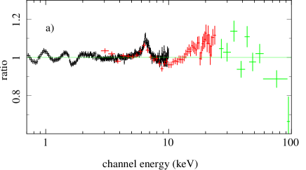
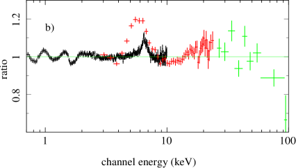
Figure 8: Residuals from simultaneous fits of the PN3col and RXTE PCA and HEXTE spectra to an absorbed power law plus disc model, excluding the 4-7 keV band. a) uses the default RXTE PCA response. b) shows the effect of including an edge at 4.78 keV with optical depth of 0.1 to account for calibration as in M06. Plainly this has a strong effect on the inferred PCA line profile. Without the edge, the PCA line is consistent with the PN but not with the piled up MOS. Conversely, with the edge the PCA line is consistent with the piled up MOS, but not with the PN.

The narrower PN line is at first sight in conflict with the consistency between 18-120s MOS data and the RXTE results. Hence we re–extract the RXTE data following M06 i.e. we use the RXTE observation ID 90118-01-06-00, extract data from all layers from PCU2, and add a systematic uncertainty of 0.6 per cent. We also extract the HEXTE data from HXT0 for the same observation, and use the same energy ranges as M06, i.e. 2.8-25.0 keV for the PCA, and 20-100 keV for HEXTE.

We illustrate our results with PN3col (the middle of the three PN spectra in terms of high energy slope). We co–fit these and the RXTE data with an absorbed disc plus power law model, excluding the 4-7 keV region. We tie all spectral parameters across all 3 instruments, but allow a variable normalisation factor. The ratio of the data to this continuum model is shown in Fig. 8a. The iron line shape is consistent between the PN and PCA data.

M06 introduce an edge at 4.78 keV, with depth $\tau=0.1$, to account for residuals sometimes seen in RXTE data at the instrumental Xe L edge. We include this edge and repeat the fit above, and obtain the residuals shown in Fig. 8b. It is clear that this has a strong impact on the derived line shape in the PCA, and on the apparent agreement with the piled up MOS data. Instead, the standard PCA response gives consistent fits with the PN spectrum.

4.2 PN-PCA: Wilkinson & Uttley 2009

We also check for consistency with WU09. They used the same PN timing data as examined here, yet their best fit model line extended down to $4R_{g}$ for an inclination of $40^{\circ}$. This was derived from approximating the ionised reflection spectrum by a laor line and neutral reflection continuum (hrefl, which does not include the reprocessed emission), and fit to the PN data extracted by excluding the central 3 columns, and background subtracting. Thus these are similar to our PN3colbgd data so we fit this spectrum together with the RXTE PCA data to reproduce the WU09 results.

We find very similar model parameters, including the broad line $R_{in}=2.5\pm 0.5~{}R_{g}$, large amount of reflection, $\Omega/2\pi=0.95\pm 0.15$ and steep continuum $1.75\pm 0.02$. This fit is formally unacceptable at $\chi^{2}_{\nu}=677/267$, but this is mainly due to the residuals noted earlier in all the PN spectra. However, it describes the overall curvature fairly well, which was all that was required in WU09 for their investigation of the variability properties.

We replace the ad hoc line plus reflection description with the reflionx model of an ionised reflector, with relativistic smearing by convolution with kdblur as above. We keep the inclination set to $40^{\circ}$ and find a much better fit $\chi^{2}=544/268$ (one fewer degrees of freedom as the line energy and intensity are set by the disc ionisation parameter). This gives a much larger inner disc radius, as the much softer shape of the reprocessed emission from ionised material twists the spectral fit so that the inferred spectral slope is much harder at $1.6$ (and $\Omega/2\pi$ much smaller), so the inferred red wing is much less prominent. This is compounded by the Compton broadening which is already present in the line from ionised material, so that the same data give $R_{in}=44~{}R_{g}$.

5 Conclusions

The detection of an extremely broad iron line in GX339-4 in M06 is an artifact of pileup in the XMM-Newton MOS data despite their efforts to mitigate the effects of this by excising the central 18” core of the image (M06, R08). We show that the MOS data are only free from the effects of pileup when such a large central core is excluded that the spectra are unusable due to systematic uncertainties in background subtraction.

The simultaneous PN data in Timing mode are much less piled up. They may still be slightly affected at the highest countrates from this variable source, though these data are mainly lost through telemetry limitations. We discuss the range of PN spectra that can be derived from these data. If there is no pileup then the full point spread function can be used, but we also excise the core in case pileup is present. We discuss whether background should be subtracted from these. Plainly background will have more effect on the lower count rate spectrum from the excised core data than from the full PSF. However, we show that the ’background’ is strongly contaminated by the source, and source photons scattered so far in the wings of the PSF are preferentially hard. Thus subtracting this ’background’ artificially steepens the spectrum at high energies.

We consider the PN spectra from the full PSF and with the core excised as representing the ranges of solutions alllowed by the data, but also fit the ’background’ subtracted PN data in order to compare with WU09. We show that all of these give a line profile which is significantly narrower than that of M06 from the MOS 18-120s data. All the PN datasets give an inner radius which is larger than the last stable orbit for a non-spinning black hole at $6R_{g}$ even for (physically unlikely) low inclination solutions, and this radius increases for (more probable) higher inclination angles for this source.

This narrower line is consistent with the RXTE PCA data, and the apparent match of the PCA with the much broader line in the MOS data of M06 is a consequence of their inclusion of an edge at 4.78 keV to account for potential deficiencies in the PCA response around the Xe L edge. The PN and RXTE data can be fit simultaneously although the telemetry limits on the PN and corelation of spectral index with luminosity means that these should have subtly different spectra. These fits give a small inner radius consistent with WU09 when fit with the same neutral reflection/ionised line model. However, this radius increases substantially when the fully self-consistent ionised reflection models are used.

Thus the PN data support the truncated disc interpretation of the low/hard state data, in direct conflict with the piled up MOS data which require that the disc extends down close to the last stable orbit of a maximally spinning black hole. Similar issues with pileup distorting the derived iron line shape have also been seen in Suzaku data of GX339-4 in an intermediate state (Yamada et al 2009). We strongly urge caution in using piled up data for detailed spectral analysis, and especially where those data are discrepant in some way with previous results.

References

- [\citeauthoryearArévalo & Uttley2006] Arévalo P., Uttley P., 2006, MNRAS, 367, 801
- [\citeauthoryearBarrio, Done, & Nayakshin2003] Barrio F. E., Done C., Nayakshin S., 2003, MNRAS, 342, 557
- [\citeauthoryearBelloni et al.2005] Belloni T., Homan J., Casella P., van der Klis M., Nespoli E., Lewin W. H. G., Miller J. M., Méndez M., 2005, A&A, 440, 207
- [\citeauthoryearBeloborodov1999] Beloborodov A. M., 1999, ApJ, 510, L123
- [\citeauthoryearBoirin & Parmar2003] Boirin L., Parmar A. N., 2003, A&A, 407, 1079
- [\citeauthoryearBoirin et al.2004] Boirin L., Parmar A. N., Barret D., Paltani S., Grindlay J. E., 2004, A&A, 418, 1061
- [\citeauthoryearBoirin et al.2005] Boirin L., Méndez M., Díaz Trigo M., Parmar A. N., Kaastra J. S., 2005, A&A, 436, 195
- [\citeauthoryearBrocksopp et al.2010] Brocksopp C., Jonker P. G., Maitra D., Krimm H. A., Pooley G. G., Ramsay G., Zurita C., 2010, arXiv, arXiv:1001.1965
- [\citeauthoryearCabanac et al.2009] Cabanac C., Fender R. P., Dunn R. J. H., Körding E. G., 2009, MNRAS, 396, 1415
- [\citeauthoryearChiang et al.2009] Chiang, C.–Y., Done C., Still M., Godot O., 2009, MNRAS, submitted, (arXiv:0911.0287)
- [\citeauthoryearDíaz Trigo et al.2006] Díaz Trigo M., Parmar A. N., Boirin L., Méndez M., Kaastra J. S., 2006, A&A, 445, 179
- [\citeauthoryearDíaz Trigo et al.2009] Díaz Trigo M., Parmar A. N., Boirin L., Motch C., Talavera A., Balman S., 2009, A&A, 493, 145
- [\citeauthoryearDone, Gierliński & Kubota2007] Done C., Gierliński M., Kubota A., 2007, A&ARv, 15, 1 (DGK07)
- [\citeauthoryearEsin, McClintock & Narayan1997] Esin A. A., McClintock J. E., Narayan R., 1997, ApJ, 489, 865
- [\citeauthoryearEsin et al.2001] Esin A. A., McClintock J. E., Drake J. J., Garcia M. R., Haswell C. A., Hynes R. I., Muno M. P., 2001, ApJ, 555, 483
- [\citeauthoryearFender et al.1999] Fender R., et al., 1999, ApJ, 519, L165
- [\citeauthoryearFerreira et al.2006] Ferreira J., Petrucci P.-O., Henri G., Saugé L., Pelletier G., 2006, A&A, 447, 813
- [\citeauthoryearGhisellini, Haardt, & Matt2004] Ghisellini G., Haardt F., Matt G., 2004, A&A, 413, 535
- [\citeauthoryearGierliński, Done, & Page2008] Gierliński M., Done C., Page K., 2008, MNRAS, 388, 753
- [\citeauthoryearGilfanov, Churazov, & Revnivtsev1999] Gilfanov M., Churazov E., Revnivtsev M., 1999, A&A, 352, 182
- [\citeauthoryearHaardt & Maraschi1993] Haardt F., Maraschi L., 1993, ApJ, 413, 507
- [\citeauthoryearHenri & Petrucci1997] Henri G., Petrucci P. O., 1997, A&A, 326, 87
- [\citeauthoryearIbragimov et al.2005] Ibragimov A., Poutanen J., Gilfanov M., Zdziarski A. A., Shrader C. R., 2005, MNRAS, 362, 1435
- [\citeauthoryearJansen et al.2001] Jansen F., et al., 2001, A&A, 365, L1
- [] Kendziorra, E, Wilms, J., Haberl, F., Kirsch, M., Martin, M., Nowak, M., 2007, XMM-SOC-CAL-TN-0073
- [\citeauthoryearKolehmainen & Done2009] Kolehmainen M., Done C., 2009, MNRAS, submitted (arXiv:0911.3281)
- [\citeauthoryearKotov, Churazov, & Gilfanov2001] Kotov O., Churazov E., Gilfanov M., 2001, MNRAS, 327, 799
- [\citeauthoryearLiu et al.2007] Liu B. F., Taam R. E., Meyer-Hofmeister E., Meyer F., 2007, ApJ, 671, 695
- [\citeauthoryearMaccarone & Coppi2002] Maccarone T. J., Coppi P. S., 2002, astro, arXiv:astro-ph/0204235
- [\citeauthoryearMakishima et al.2008] Makishima K., et al., 2008, PASJ, 60, 585
- [\citeauthoryearMalzac, Dumont, & Mouchet2005] Malzac J., Dumont A. M., Mouchet M., 2005, A&A, 430, 761
- [\citeauthoryearMarkoff, Nowak, & Wilms2005] Markoff S., Nowak M. A., Wilms J., 2005, ApJ, 635, 1203
- [\citeauthoryearMiller et al.2006] Miller J. M., Homan J., Steeghs D., Rupen M., Hunstead R. W., Wijnands R., Charles P. A., Fabian A. C., 2006, ApJ, 653, 525 (M06)
- [\citeauthoryearMiniutti et al.2003] Miniutti G., Fabian A. C., Goyder R., Lasenby A. N., 2003, MNRAS, 344, L22
- [\citeauthoryearMiniutti & Fabian2004] Miniutti G., Fabian A. C., 2004, MNRAS, 349, 1435
- [\citeauthoryearMiyamoto & Kitamoto1989] Miyamoto S., Kitamoto S., 1989, Natur, 342, 773
- [\citeauthoryearPoutanen & Fabian1999] Poutanen J., Fabian A. C., 1999, MNRAS, 306, L31
- [\citeauthoryearReis et al.2008] Reis R. C., Fabian A. C., Ross R. R., Miniutti G., Miller J. M., Reynolds C., 2008, MNRAS, 387, 1489 (R08)
- [\citeauthoryearReis, Miller, & Fabian2009] Reis R. C., Miller J. M., Fabian A. C., 2009, MNRAS, 395, L52
- [\citeauthoryearRemillard & McClintock2006] Remillard R. A., McClintock J. E., 2006, ARA&A, 44, 49
- [\citeauthoryearRevnivtsev, Gilfanov, & Churazov1999] Revnivtsev M., Gilfanov M., Churazov E., 1999, A&A, 347, L23
- [\citeauthoryearRoss & Fabian2005] Ross R. R., Fabian A. C., 2005, MNRAS, 358, 211
- [\citeauthoryearRykoff et al.2007] Rykoff E. S., Miller J. M., Steeghs D., Torres M. A. P., 2007, ApJ, 666, 1129
- [\citeauthoryearSidoli et al.2001] Sidoli L., Oosterbroek T., Parmar A. N., Lumb D., Erd C., 2001, A&A, 379, 540
- [\citeauthoryearSim et al.2010] Sim S. A., Miller L., Long K. S., Turner T. J., Reeves J. N., 2010, arXiv, arXiv:1002.0544
- [\citeauthoryearStern et al.1995] Stern B. E., Begelman M. C., Sikora M., Svensson R., 1995, MNRAS, 272, 291
- [\citeauthoryearStrüder et al.2001] Strüder L., et al., 2001, A&A, 365, L18
- [\citeauthoryearTitarchuk, Laurent, & Shaposhnikov2009] Titarchuk L., Laurent P., Shaposhnikov N., 2009, ApJ, 700, 1831
- [\citeauthoryearTomsick2008] Tomsick J. A., 2008, mqw..conf, 4, (arXiv:0812.2980)
- [\citeauthoryearTomsick et al.2009] Tomsick J. A., Yamaoka K., Corbel S., Kaaret P., Kalemci E., Migliari S., 2009, ApJ, 707, L87
- [\citeauthoryearTurner et al.2001] Turner M. J. L., et al., 2001, A&A, 365, L27
- [\citeauthoryearYamada et al.2009] Yamada, et al., 2009, Ap. J., submitted
- [\citeauthoryearWilkinson & Uttley2009] Wilkinson T., Uttley P., 2009, MNRAS, 397, 666