AMiBA: SCALING RELATIONS BETWEEN THE INTEGRATED COMPTON-$y$ AND X-RAY DERIVED TEMPERATURE, MASS, AND LUMINOSITY

Abstract

We investigate the scaling relations between the X-ray and the thermal Sunyaev–Zel’dovich Effect (SZE) properties of clusters of galaxies, using data taken during 2007 by the Y.T. Lee Array for Microwave Background Anisotropy (AMiBA) at 94 GHz for the six clusters A1689, A1995, A2142, A2163, A2261, and A2390. The scaling relations relate the integrated Compton-$y$ parameter $Y_{2500}$ to the X-ray derived gas temperature $T_{\textrm{e}}$, total mass $M_{2500}$, and bolometric luminosity $L_{X}$ within $r_{2500}$. Our results for the power-law index and normalization are both consistent with the self-similar model and other studies in the literature except for the $Y_{2500}$–$L_{X}$ relation, for which a physical explanation is given though further investigation may be still needed. Our results not only provide confidence for the AMiBA project but also support our understanding of galaxy clusters.

1. INTRODUCTION

The Sunyaev–Zel’dovich Effect (SZE) is a powerful tool that can potentially answer long-standing questions about the large-scale distribution of matter. The SZE is a spectral distortion of the cosmic microwave background (CMB), induced when a fraction of CMB photons are scattered by hot electrons in the cores of massive galaxy clusters (Sunyaev & Zel’dovich, 1970). The redshift independence of the SZE enables the direct detection of distant clusters without the $(1+z)^{4}$ surface brightness dimming that limits other techniques, including X-ray observations. Clusters studied via the SZE are therefore effective cosmological probes. Studying their properties in detail will lead to heightened understanding of the mass power spectrum, and should provide improved constraints on cosmological parameters.

In the simplest scenario, where gravity is assumed to be the only influence on the formation of galaxy clusters, a simple ‘self-similar’ model can be used to relate the physical properties of clusters (Kaiser, 1986). Assuming spherical collapse of the dark matter (DM) halo, and hydrostatic equilibrium of gas in the DM gravitational potential, one can derive power-law scaling relations between various X-ray and SZE quantities, e.g. luminosity and temperature, gas mass and temperature, total mass and luminosity, entropy and temperature, and Compton-$y$ parameter and temperature. Existence of these relations in observations can be seen in, for example, Mushotzky & Scharf (1997); Benson et al. (2004); Bonamente et al. (2008); Morandi et al. (2007). These relations are also found in numerical simulations, e.g., between X-ray quantities (Nagai et al., 2007), SZE flux and total mass or gas mass (Motl et al., 2005; Nagai, 2006), and integrated Compton-$y$ and temperature or luminosity (da Silva et al., 2004). Deviations from the scaling relations should reveal the importance of non-gravitational processes for the formation of clusters (e. g.  Allen & Fabian, 1998; McCarthy et al., 2002, 2003a), or constrain the mass distributions of clusters (Reiprich & Böhringer, 2002). Furthermore, the scaling relations can be used as an utility to extract important quantities and evolution behaviors for remote clusters using SZE observables alone.

The Y.T. Lee Array for Microwave Background Anisotropy (AMiBA) experiment (Ho et al., 2009) observed and detected the SZEs of six massive Abell clusters in the range $0.09<z<0.32$ during the year 2007 (Wu et al., 2009). AMiBA is a coplanar interferometer that during 2007 operated at 94 GHz with seven 0.6-m antennas in a hexagonal close-packed configuration, giving a synthesized resolution of about $6\arcmin$. The array has a sensitivity of 63 mJy/hr for on-source integration, and an overall efficiency of $0.36$ (Lin et al., 2009). Details for the transformation of the raw data into calibrated visibilities are presented in Wu et al. (2009), and the checks on data integrity are described in Nishioka et al. (2009). At our observing frequency the SZE signal is an intensity decrement in the CMB. We fit the central (peak) decrement in the AMiBA visibilities using isothermal $\beta$-models (Cavaliere & Fusco-Femiano, 1976), taking account of contamination from the primary CMB and foreground emissions (Liu et al., 2009). Other companion papers include Chen et al. (2009) and Koch et al. (2009a), where the technical aspects of the instruments are described, Umetsu et al. (2009), where the AMiBA SZE data is combined with weak lensing data from Subaru to analyze the distributions of mass and hot baryons, Koch et al. (2009b), where the Hubble constant is estimated from AMiBA SZE and X-ray data, and Molnar et al. (2009), which discusses the feasibility of further constraining the intra-cluster gas model using AMiBA upgraded to 13 antennas (Ho et al., 2009, AMiBA13). The consistency of our results with other observations and theoretical expectations will validate not only the performance and capability of instruments, but also the analysis methodology. Since AMiBA is one of few leading SZE instruments operating at 3-mm wavelength, we anticipate that it will fill an important role by providing 3-mm SZE data for spectral studies.

In this article we address the scaling relations between the integrated SZE Compton-$y$ parameter obtained by AMiBA and X-ray gas temperature, X-ray luminosity, and total cluster mass derived from the literature. In Section 2 we discuss the cluster gas models and cluster parameters derived from the X-ray data. In Section 3 we calculate the integrated Compton-$y$ parameter for each of the six clusters. In Section 4 we investigate the scaling relations including the consideration for errors. We further discuss our results in Section 5 and draw conclusions in Section 6.

2. CLUSTER PROPERTIES FROM X-RAY DATA

As the $u$–$v$ coverage is incomplete for a single interferometric SZE experiment, we can not measure the accurate profile of a cluster or its central intensity. Therefore we have chosen to assume a cluster model, and thus a flux-density profile, so that a corresponding template in $u$–$v$ space can be fitted to the observed visibilities in order to estimate the underlying model parameters including the central SZE intensity, $\Delta I_{0}$. We apply the spherical isothermal $\beta$-model in our X-ray and SZE analysis. The cluster gas density distribution is of the form

$$n_{\mathrm{e}}(r)=n_{\mathrm{e}0}\left(1+\frac{r^{2}}{r_{\mathrm{c}}^{2}}\right)^{-3\beta/2}\quad,$$ (1)

where $n_{\mathrm{e}0}$ is the central number density of electrons, $r$ is the radius from the cluster center, $r_{\mathrm{c}}$ the core radius and $\beta$ is a structure index. Due to the limited resolution of AMiBA in its 7-element closed-packed configuration, we cannot obtain good estimates for some of the model parameters from our SZE data alone. Therefore we have taken the X-ray derived values for $\beta$ and $\theta_{\mathrm{c}}$ from the literature, where $\theta_{\mathrm{c}}=r_{\mathrm{c}}/D_{\mathrm{A}}$ and $D_{\mathrm{A}}$ is the angular diameter distance. Throughout this paper, we assume a flat $\Lambda$CDM universe with $H_{0}=70$ km $\mathrm{s}^{-1}\mathrm{Mpc}^{-1}$, $\Omega_{\mathrm{M}}=0.3$, and $\Omega_{\Lambda}=0.7$.

To relate with the SZE Compton-$y$ parameter, we also need to borrow the cluster gas temperature $T_{\mathrm{e}}$, the total mass $M_{2500}$, and the bolometric luminosity $L_{\mathrm{X}}$ derived from the X-ray data. $M_{2500}$ refers to the total mass in a cluster central region out to $r=r_{2500}$, defined as the radius of mean overdensity $2500\times\rho_{\mathrm{c}}$ where $\rho_{\mathrm{c}}$ is the critical density at redshift $z$. Given $\beta$, $r_{\mathrm{c}}$ and $T_{\mathrm{e}}$ for a cluster, we can compute first $r_{2500}$ and then $M_{2500}$ through the total mass equation of the $\beta$-model (Grego et al., 2001)

$$M_{2500}=2500\frac{4\pi}{3}r_{2500}^{3}\rho_{\mathrm{c}}=\frac{3\beta k_{\textrm{B}}T_{\mathrm{e}}}{G\mu m_{p}}\frac{r_{2500}^{3}}{r_{\mathrm{c}}^{2}+r_{2500}^{2}}\quad,$$ (2)

where $\mu=0.6$ is the mean molecular weight in units of $m_{\mathrm{H}}$ for an assumed near-solar metallicity of the intracluster medium.

We considered two sets of X-ray derived parameters. The first set is mainly based on the Chandra data, and this leads to our main results. The second set is mainly derived from ROSAT images or a combination of ROSAT data and ASCA spectral measurements (the ASCA/ROSAT parameters in what follows). Because these data are generally of lower accuracy, we include them only for comparison.

2.1. Chandra

To deal with the complicated non-gravitational physics in cluster cores, including radiative cooling and feedback mechanisms, and the transient boosting of surface brightness and spectral temperature during merging events, the parameters of the Chandra set were derived by fitting an isothermal $\beta$-model to the X-ray data with the central 100 kpc excised. The most recent and currently most extensive studies of $H_{0}$ (Bonamente et al., 2006) and the gas mass fraction $f_{\mathrm{gas}}$ (LaRoque et al., 2006) adopted this 100-kpc cut model in their analysis, and claim that a cut at 100 kpc is large enough to exclude the cooling region in cool-core clusters while retaining sufficient photons for modeling. This model was also used in recent studies of scaling relations based on X-ray and SZE observations (Morandi et al., 2007; Bonamente et al., 2008).

Table 2.2 summarizes the parameters from Chandra observations, and the values of $r_{2500}$ and $M_{2500}$ derived from them. Note that Chandra-based values of $\beta$ and $\theta_{\mathrm{c}}$ for A2142 are unavailable in the literature, and so we adopted values taken from the ASCA/ROSAT set, which were not determined by fitting the 100-kpc cut model. The gas temperature for A2142 is Chandra-based, as given by Markevitch et al. (2000). The temperature fit allowed a cooling component to be present, but was based on the overall X-ray spectrum of A2142, rather than discarding photons extracted from the central 100 kpc region. Nevertheless, if A2142 is excluded from the sample for this set of parameters, it has only a minor effect on the scaling relations (less than a $5\%$ change for the power index or the normalization; see Sec. 4).

The values of $\beta$ and $\theta_{\mathrm{c}}$ for A2390 are taken from Allen et al. (2001) who fit the X-ray surface brightness profile to an isothermal $\beta$-model between radii $80$ and $900$ kpc. As the authors remark, however, an isothermal $\beta$-model ignoring the central region associated with the possible cooling flow cannot describe the mass distribution well, since there is a ‘break’ in the surface brightness profile at $r\sim 500$ kpc. A better fit can be obtained using a simple broken power-law model, or assuming an NFW (Navarro et al., 1997) potential with the assumption of gas isothermality relaxed.

2.2. ASCA/ROSAT

Parameters derived from ASCA and ROSAT are summarized in Table 2.2. The gas temperatures and the bolometric luminosities of our clusters, except A1995 and A2163, are compiled by Allen & Fabian (1998) and Allen (2000), where the X-ray spectra were fitted by using a model with an isothermal plasma in collisional equilibrium, including an additional component explicitly to account for cooling flows (Model C). For A2163, which is not a cooling-core cluster, we take the values from the same papers, but without the additional cooling component (Model A). For A1995, which is absent from these papers, we use the value of $T_{\mathrm{e}}$ from Patel et al. (2000), who detected no excess in the X-ray surface brightness biased from a cooling flow in the cluster center. However, A1995 has recently been classified as a cooling cluster, according to the criterion that the cooling time in the central inner region is less than the Hubble time at the cluster redshift (Morandi et al., 2007).

All values in Tables 2.2 and 2.2 are presented at the $68.3\%$ confidence level. Errors are obtained by propagating the errors in the input parameters from the literature through a Monte-Carlo process.

Table 1Cluster parameters of the Chandra set

	$z$	$\beta$	$\theta_{\mathrm{c}}$	$r_{2500}$	$T_{\mathrm{e}}$	$M_{2500}$	$L_{\mathrm{X}}$	ref
Cluster			(″)	(kpc)	(keV)	($10^{14}M_{\sun}$)	($10^{45}$ erg/s)	($\beta$ & $\theta_{\mathrm{c}}$, $T_{\mathrm{e}}$, $L_{\mathrm{X}}$)
A1689	$0.183$	$0.686_{-0.01}^{+0.01}$	$48.0_{-1.7}^{+1.5}$	$607_{-23}^{+22}$	$8.72_{-0.56}^{+0.63}$	$3.82_{-0.42}^{+0.43}$	$3.15\pm 0.09$	1, 4, 4
A1995	$0.322$	$0.923_{-0.023}^{+0.021}$	$50.4_{-1.5}^{+1.4}$	$579_{-21}^{+21}$	$7.56_{-0.41}^{+0.45}$	$3.87_{-0.41}^{+0.43}$	$1.51\pm 0.05$	1, 4, 4
A2142	$0.089$	$0.74_{-0.01}^{+0.01}$	$188.4_{-13.2}^{+13.2}$	$608_{-31}^{+30}$	$8.80_{-0.55}^{+0.73}$	$3.49_{-0.52}^{+0.53}$	–	2, 5, –
A2163	$0.202$	$0.700_{-0.07}^{+0.07}$	$78.8_{-0.6}^{+0.6}$	$684_{-41}^{+40}$	$12.0_{-0.26}^{+0.28}$	$5.59_{-0.96}^{+1.00}$	$4.80\pm 0.05$	1, 4, 4
A2261	$0.224$	$0.628_{-0.02}^{+0.03}$	$29.2_{-2.9}^{+4.8}$	$531_{-22}^{+22}$	$7.47_{-0.47}^{+0.53}$	$2.67_{-0.32}^{+0.33}$	$2.02\pm 0.07$	1, 4, 4
A2390	$0.233$	$0.58_{-0.058}^{+0.058}$	$43.3_{-4.33}^{+4.33}$	$583_{-33}^{+32}$	$10.18_{-0.21}^{+0.23}$	$3.57_{-0.58}^{+0.61}$	$4.66\pm 0.05$	3, 4, 4

References. — (1) Bonamente et al. (2006). (2) Sanderson & Ponman (2003); Lancaster et al. (2005). (3) Allen et al. (2001) with a $10\%$ error assumed. (4) Morandi et al. (2007). (5) Markevitch et al. (2000).

Table 2Cluster parameters of the ASCA/ROSAT set

	$z$	$\beta$	$\theta_{\mathrm{c}}$	$r_{2500}$	$T_{\mathrm{e}}$	$M_{2500}$	$L_{\mathrm{X}}$	ref
Cluster			(″)	(kpc)	(keV)	($10^{14}M_{\sun}$)	($10^{45}$ erg/s)	($\beta$ & $\theta_{\mathrm{c}}$, $T_{\mathrm{e}}$, $L_{\mathrm{X}}$)
A1689	$0.183$	$0.609_{-0.005}^{+0.005}$	$26.6_{-0.7}^{+0.7}$	$625_{-20}^{+19}$	$10.0_{-0.49}^{+0.73}$	$4.17_{-0.38}^{+0.39}$	$6.26$	1, 4, 4
A1995	$0.322$	$0.770_{-0.063}^{+0.117}$	$38.9_{-4.3}^{+6.9}$	$579_{-48}^{+47}$	$8.59_{-0.67}^{+0.86}$	$3.88_{-0.91}^{+1.00}$	–	1, 5, –
A2142	$0.089$	$0.74_{-0.01}^{+0.01}$	$188.4_{-13.2}^{+13.2}$	$629_{-29}^{+28}$	$9.3_{-0.43}^{+0.79}$	$3.87_{-0.51}^{+0.53}$	$6.78$	2, 4, 4
A2163	$0.202$	$0.674_{-0.008}^{+0.011}$	$87.5_{-2.0}^{+2.5}$	$716_{-15}^{+15}$	$13.83_{-0.45}^{+0.47}$	$6.37_{-0.41}^{+0.42}$	$14.7$	1, 4, 4
A2261	$0.224$	$0.516_{-0.013}^{+0.014}$	$15.7_{-1.1}^{+1.2}$	$589_{-71}^{+66}$	$10.9_{-1.34}^{+3.59}$	$3.68_{-1.20}^{+1.31}$	$5.83$	1, 4, 4
A2390	$0.233$	$0.6_{-0.06}^{+0.06}$	$28_{-2.8}^{+2.8}$	$721_{-174}^{+155}$	$14.5_{-3.16}^{+9.42}$	$7.09_{-4.14}^{+5.02}$	$10.11$	3, 4, 4

References. — (1) Reese et al. (2002). (2) Sanderson & Ponman (2003); Lancaster et al. (2005). (3) Böhringer et al. (1998) with a $10\%$ error assumed. (4) Allen (2000). (5) Patel et al. (2000).

3. CLUSTER PROPERTIES FROM SZE

In AMiBA targeted observations at 94 GHz, the sky signal is dominated by the thermal SZE. The amplitude of such signals is proportional to the Compton-$y$ parameter, $y=\sigma_{T}/\left(m_{\mathrm{e}}c^{2}\right)\int_{0}^{\infty}k_{\textrm{B}}T_{\mathrm{e}}(l)n_{\mathrm{e}}(l)\>dl$ where $\sigma_{T}$ is the Thomson scattering cross section, $k_{\textrm{B}}T_{\mathrm{e}}(l)n_{\mathrm{e}}(l)$ is the electron pressure, and the integral is taken along the line of sight. The Compton-$y$ parameter can be interpreted as a measure of Comptonization integrated through a cluster. In terms of a change in intensity, the thermal SZE observed at frequency $\nu$ can be represented by a decrement

$$\Delta I_{\textrm{SZE}}=y\cdot g\left(x,T_{\mathrm{e}}\right)\cdot I_{\textrm{CMB}}\,,$$ (3)

where $x\equiv h\nu/\left(k_{\textrm{B}}T_{\textrm{CMB}}\right)$, $T_{\textrm{CMB}}=2.725$ K (Mather et al., 1999), and $I_{\textrm{CMB}}\equiv 2h\nu^{3}\mathrm{c}^{-2}\left(e^{x}-1\right)^{-1}$ is the CMB intensity. The factor $g\left(x,T_{\mathrm{e}}\right)$ can be expressed as (Bonamente et al., 2008; Morandi et al., 2007; Udomprasert et al., 2004)

$$g\left(x,T_{\mathrm{e}}\right)=\frac{xe^{x}}{e^{x}-1}\left(F-4\right)+\delta_{\textrm{rel}}\left(x,T_{\mathrm{e}}\right),$$ (4)

where $\delta_{\textrm{rel}}\left(x,T_{\mathrm{e}}\right)$ is a small relativistic correction (Challinor & Lasenby, 1998)

$$\begin{split}\delta_{\textrm{rel}}\left(x,T_{\mathrm{e}}\right)&=\frac{xe^{x}}{e^{x}-1}\frac{k_{\textrm{B}}T_{\mathrm{e}}}{m_{\mathrm{e}}c^{2}}\Bigl{[}-10+\frac{47}{2}F-\frac{42}{5}F^{2}+\\ &\quad\frac{7}{10}F^{3}+\frac{7}{5}G^{2}(-3+F)\Bigr{]},\end{split}$$ (5)

$F\equiv x\coth(x/2)$, and $G\equiv x/\sinh(x/2)$. The relativistic correction is about $6\%$ for $\nu=94$ GHz and $T_{\mathrm{e}}=10$ keV, which is a typical temperature for our SZE clusters.

Given a gas density profile $n_{\mathrm{e}}(r)$ we can determine the distribution of $\Delta I_{\textrm{SZE}}$ on the plane of the sky. For an isothermal $\beta$-model, the projected SZE decrement distribution has a simple analytical form (e.g. Udomprasert et al., 2004)

$$\Delta I_{{\rm SZE}}(\theta)=\Delta I_{0}\left(1+\frac{\theta^{2}}{\theta_{\mathrm{c}}^{2}}\right)^{(1-3\beta)/2},$$ (6)

where $\theta$ and $\theta_{\mathrm{c}}$ are the angular equivalents of $r$ and $r_{\mathrm{c}}$ respectively, and $\Delta I_{0}$ is the central SZE intensity decrement. Because the SZE clusters are not well resolved by AMiBA, we cannot get a good estimate of $\Delta I_{0}$, $\beta$, and $\theta_{\mathrm{c}}$ simultaneously from our data alone. Instead, we adopt the X-ray derived values for $\beta$ and $\theta_{\mathrm{c}}$ from Chandra or ASCA/ROSAT, and then estimate $\Delta I_{0}$ (Liu et al., 2009) by fitting the $\beta$-model to the SZE visibilities obtained in Wu et al. (2009).

For the two different sets of X-ray parameters we accordingly obtain two sets of $\Delta I_{0}$ values. For the the Chandra set with a 100 kpc-cut model we choose to fit the entire SZE data, while using the X-ray parameters from the same model. LaRoque et al. (2006) and Bonamente et al. (2006) already remarked that there is no simple way to mask the central 100 kpc from the interferometric SZE data because these data are in the $u$–$v$ space. Nevertheless, our approach should be valid because the limited resolution of the current AMiBA is insensitive to the details of the cluster core. Moreover, since the SZE probes the integrated gas pressure, which is linear in $n_{\mathrm{e}}$, the parameters derived from the SZE data should be less dependent on the core properties than parameters derived from X-ray observations, where the X-ray surface brightness $\propto n_{\mathrm{e}}^{2}$. Table 3 summarizes the resulting estimated values of $\Delta I_{0}$ based on Chandra. We note that the effects of foregrounds such as radio source contamination, Galactic emission, and confusion from primary CMB fluctuations have been taken into account (Liu et al., 2009).

In addition to the intensity decrement, the thermal SZE also can be expressed in terms of a change of the thermodynamic temperature of the CMB, $\Delta T_{\textrm{SZE}}=y\cdot g\left(x,T_{\mathrm{e}}\right)\left(e^{x}-1\right)(xe^{x})^{-1}\cdot T_{\textrm{CMB}}$ (e.g., Bonamente et al., 2008). Thus for a cluster observed at a given frequency, the $\Delta I_{\textrm{SZE}}$ (Eq. (3)) and $\Delta T_{\textrm{SZE}}$ are equivalent measures of the Compton-$y$ parameter. In Table 3, we include the values of the central thermodynamic temperature decrement $\Delta T_{0}$ that correspond to the $\Delta I_{0}$ based on Chandra.

To obtain an overall measure of the thermal energy content in a cluster, we computed the integrated Compton-$y$ parameter $Y_{2500}$, which is the Compton-$y$ integrated from its center out to the projected radius $r_{2500}$,

$$\begin{split}Y_{2500}&\equiv\int_{\Omega_{2500}}y\>d\Omega\\ &=\frac{2\pi\Delta I_{0}}{I_{\textrm{CMB}}\,g(x,T_{\mathrm{e}})}\int_{0}^{r_{2500}/D_{\mathrm{A}}}\left(1+\frac{\theta^{2}}{\theta_{\mathrm{c}}^{2}}\right)^{(1-3\beta)/2}\theta d\theta,\end{split}$$ (7)

where $\Omega$ is the solid angle of the integrated patch and $\Omega_{2500}$ is the total value covered within radius $r_{2500}$. The integrated Compton-$y$ parameter has been shown to be a more robust quantity than the central value of Compton-$y$ for observational tests, because it is less dependent on the model of gas distribution used for the analysis (Benson et al., 2004). In addition, integrating the Compton-$y$ out to a large projected radius diminishes (though does not completely remove) effects resulting from the presence of strong entropy features in the central regions of clusters (McCarthy et al., 2003a). Table 3 summarizes our derived values of $Y_{2500}$, adopting the parameters based on Chandra. In Section 4, the $Y_{2500}$ derived from both X-ray parameter sets will be considered for its scaling relationship with $T_{\mathrm{e}}$, $M_{2500}$ and $L_{\mathrm{X}}$.

Although using X-ray data to determine the shapes of cluster SZE profiles is a common strategy in SZE analysis, it has been shown that this will bias the results of fitted parameters due to the assumption of isothermality of a $\beta$-model (e.g.  Komatsu & Seljak, 2001; Hallman et al., 2007). In Section 5 we will further discuss this issue, and apply a simple correction to our results based on the work of Hallman et al. (2007).

AMiBA is one of the first instruments to provide 3-mm SZ detections of the cluster targets, expanding our knowledge of the SZE spectra for clusters. Table 3 compares our results for $Y_{2500}$ at 94 GHz with results at other frequencies: the BIMA/OVRO results at 30 GHz (McCarthy et al., 2003b; Morandi et al., 2007), and the SuZIE II results at 145 GHz (Benson et al., 2004). We have converted the BIMA/OVRO values of integrated Compton-$y$ parameter, $y_{2500}$ (Morandi et al., 2007), to our $Y_{2500}$ using $Y_{2500}=y_{2500}\,(F-4)\,xe^{x}/\left[(e^{x}-1)\,I_{0}\,g(x,T_{\mathrm{e}})\right]$ where $I_{0}\equiv 2\left(k_{\mathrm{B}}T_{\mathrm{CMB}}\right)^{3}(h\mathrm{c})^{-2}$, and $x$, $F$, and $g(x,T_{\mathrm{e}})$ are defined in Eq. (4) with frequency $\nu=30$ GHz. For SuZIE II, $Y_{2500}$ is obtained from $Y_{2500}=S\left(r_{2500}\right)/\left[I_{\mathrm{CMB}}\,g(x,T_{\mathrm{e}})\right]$, where $S\left(r_{2500}\right)$ is the integrated SZ flux defined in Benson et al. (2004), and $I_{\mathrm{CMB}}$ and $g(x,T_{\mathrm{e}})$ are calculated at $\nu=30$ GHz. All three sets of results are based on reconstruction of the gas profile of the clusters using an isothermal $\beta$-model, and all include the relativistic correction in their estimates of $Y_{2500}$. Our results are consistent with those from BIMA/OVRO except for A1995, and can be seen to be generally lower than those from SuZIE II.

Since $Y_{2500}$ is relatively insensitive to cluster morphology and the thermal structure of the intracluster medium, the difference between the results for A1995 could mostly come from the different SZ techniques. The AMiBA data led to a signal-to-noise ratio of about 6, based on an integration time of about 5.5 hours. A1995 is a relatively low-mass, cool, cluster and hence produces a smaller SZE than the other clusters in our sample. This causes the statistical significance of the different values for $Y_{2500}$ to be low, and that differing residual contamination by point sources and primary CMB fluctuations (Liu et al., 2009) could be an important factor. Further multi-frequency studies of A1995 are needed to improve the result for the SZE of this cluster.

Table 3Parameters of AMiBA clusters derived from SZE observations

	$\Delta I_{0}$	$\Delta T_{0}$	$Y_{2500}$ ($10^{-10}$ sr)
Cluster	($10^{5}$Jy/sr)	(mK)	BIMA/OVRO	AMiBA	SuZIE II
A1689	$-2.36\pm 0.71$	$-0.40\pm 0.12$	$2.17\pm 0.14$	$2.82\pm 0.86$	$4.65_{-0.51}^{+0.61}$
A1995	$-3.19\pm 1.23$	$-0.54\pm 0.21$	$0.71\pm 0.06$	$1.49\pm 0.58$	–
A2142	$-2.09\pm 0.36$	$-0.35\pm 0.06$	–	$13.44\pm 2.40$	–
A2163	$-3.64\pm 0.61$	$-0.62\pm 0.10$	$5.53\pm 0.41$	$6.61\pm 1.38$	$5.50_{-0.70}^{+0.76}$
A2261	$-2.59\pm 0.90$	$-0.44\pm 0.15$	$1.51\pm 0.18$	$1.72\pm 0.64$	$4.46_{-0.94}^{+1.70}$
A2390	$-2.85\pm 0.77$	$-0.48\pm 0.13$	–	$3.12\pm 0.98$	$3.69_{-0.57}^{+0.56}$

Note. — The integrated Compton parameters $Y_{2500}$ measured by AMiBA (94 GHz) are compared with results from BIMA/OVRO (30 GHz; McCarthy et al., 2003b; Morandi et al., 2007) and SuZIE II (145 GHz; deduced from Benson et al., 2004). The central SZE intensity $\Delta I_{0}$, its corresponding thermodynamic temperature decrement $\Delta T_{0}$, and the AMiBA $Y_{2500}$ were derived using the Chandra-based parameters. Isothermal $\beta$-models are used in all three sets of observation to reconstruct the gas profile of clusters and derive $Y_{2500}$. The relativistic correction $\delta_{\textrm{rel}}\left(x,T_{\mathrm{e}}\right)$ in Eq. (5) is also taken into account in all three cases. Errors are given at the $68.3\%$ confidence level.

4. SCALING RELATIONS

4.1. Theoretical Expectations

In the context of the self-similar model, if assuming hydrostatic equilibrium and an isothermal distribution of baryons in the spherically-collapsed DM halo, it can be shown that there are simple power-law scaling relations between the SZE and X-ray quantities. Specifically there are simple relations between the integrated Comptonization and the gas temperature $T_{\mathrm{e}}$, the cluster total mass $M_{tot}$ and the bolometric X-ray luminosity $L_{\mathrm{X}}$,

$$YD_{\mathrm{A}}^{2} \propto T_{\mathrm{e}}^{5/2}E(z)^{-1},$$ (8)

$$YD_{\mathrm{A}}^{2} \propto M_{tot}^{5/3}E(z)^{2/3},$$ (9)

$$YD_{\mathrm{A}}^{2} \propto L_{\mathrm{X}}^{5/4}E(z)^{-9/4},$$ (10)

where $E^{2}(z)=\Omega_{\mathrm{M}}(1+z)^{3}+\Omega_{\Lambda}+\Omega_{\mathrm{k}}(1+z)^{2}$ (Morandi et al., 2007). We note that these scaling relations assume that the fraction of the cluster mass present as gas, $f_{{\rm gas}}$, is a constant. Bonamente et al. (2008) found no significant scatter of $f_{gas}$ in their results. Nevertheless, recent X-ray work in observations (e.g. Vikhlinin, 2006) and simulations (Kravtsov et al., 2005) suggest that some variation may be expected.

Following standard method (e.g. Press et al., 2002), we perform a linear least-squares fitting in $\log_{10}$ space, $\log_{10}(y)=A+B\log_{10}(x)$, taking account of errors in both $x$ and $y$, to estimate the normalization $A$ and power law index $B$ of each scaling relation. The $\chi^{2}$ statistic is defined as

$$\chi^{2}=\sum\frac{\left(\log_{10}(y_{i})-A-B\log_{10}(x_{i})\right)^{2}}{\left(\sigma_{y_{i}}\log_{10}(e)/y_{i}\right)^{2}+\left(B\sigma_{x_{i}}\log_{10}(e)/x_{i}\right)^{2}}\quad,$$ (11)

and is minimized as in Benson et al. (2004, Eq. (13)). $\sigma_{y_{i}}$ and $\sigma_{x_{i}}$ for the sample points are obtained from the upper and lower uncertainties around the best-fit values as $\sigma=\left(\sigma^{+}+\sigma^{-}\right)/2$. The number of degrees of freedom (d.o.f.) is $N-2$ with $N$ equal to the total number of clusters in the sample. $1\sigma$ errors in $A$ and $B$ are determined by projecting the $\Delta\chi^{2}=1$ contour on each coordinate axis.

4.2. Derived Observational Results

The results of fitting $\log_{10}(y)=A+B\log_{10}(x)$ for each scaling relation are summarized in Table 4. Figures 1, 2, and 3 show our sample of six clusters and the best-fitting scaling relations. Each figure shows the scaling results based on the Chandra and the ASCA/ROSAT parameters, for comparison. Five of the six clusters in our sample are cooling-core (CC) clusters; the exception is cluster A2163, which is of non-cooling core (NCC) type (Myers et al., 1997; Allen, 2000; McCarthy et al., 2003b; Morandi et al., 2007).

Table 4Scaling relations from X-ray and AMiBA SZE data

$\log_{10}(y)=A+B\log_{10}(x)$			Chandra				ASCA/ROSAT
$x$	$y$		$A$	$B$	$\chi_{\mathrm{min}}^{2}$(d.o.f.)		$A$	$B$	$\chi_{\mathrm{min}}^{2}$(d.o.f.)
$T_{\mathrm{e}}$/keV	$Y_{2500}D_{\mathrm{A}}^{2}E(z)/{\rm Mpc^{2}}$		$-5.94_{-0.72}^{+0.67}$	$2.28_{-0.68}^{+0.73}$	$1.43(4)$		$-5.97_{-0.78}^{+0.67}$	$2.21_{-0.64}^{+0.74}$	$3.36(4)$
$M_{2500}/10^{14}M_{\sun}$	$Y_{2500}D_{\mathrm{A}}^{2}E(z)^{-2/3}/{\rm Mpc^{2}}$		$-4.82_{-0.59}^{+0.39}$	$1.71_{-0.64}^{+1.01}$	$1.82(4)$		$-5.03_{-0.60}^{+0.43}$	$1.90_{-0.61}^{+0.83}$	$1.95(4)$
$L_{\mathrm{X}}/10^{45}{\rm erg\,s^{-1}}$	$Y_{2500}D_{\mathrm{A}}^{2}E(z)^{9/4}/{\rm Mpc^{2}}$		$-4.05_{-0.18}^{+0.18}$	$0.77_{-0.32}^{+0.32}$	$6.15(3)$		$-4.69_{-0.28}^{+0.28}$	$1.11_{-0.29}^{+0.28}$	$1.69(3)$

Note. — The $Y_{2500}-L_{\mathrm{X}}$ fit uses only five clusters, omitting A2142 in the Chandra set and omitting A1995 in the ASCA/ROSAT set. $\chi_{\mathrm{min}}^{2}$ gives the minimum value of $\chi^{2}$, as defined in Eq. (11), with the corresponding number of degrees of freedom (d.o.f.). Errors are given at the $68.3\%$ confidence level.

4.2.1 The $Y_{2500}$ –$T_{\mathrm{e}}$ relation

Our results for the power law index $B$ from both sets of X-ray parameters agree with the self-similar model $B=2.5$ at the $1\sigma$ level. They are also consistent with the values of $B=2.37\pm 0.23$ from BIMA/OVRO (Bonamente et al., 2008), $B=2.21\pm 0.41$ from SuZIE II (Benson et al., 2004), and $B=2.64\pm 0.28$ (CC+NCC sample) and $B=2.74\pm 0.23$ (CC sample only) from Morandi et al. (2007).

To compare the normalization in scaling relations in the same analytic form and units, we convert the SuZIE II normalizations to $A=A^{\prime}-\log_{10}\left[I_{0}\,g(x,T_{\mathrm{e}})x^{3}(e^{x}-1)^{-1}\right]$, where $I_{0}\equiv 2\left(k_{\textrm{B}}T_{\textrm{CMB}}\right)^{3}\left(h\mathrm{c}\right)^{-2}$, $x$ is calculated at the SuZIE II observing frequency of 145 GHz, and the primes stand for the power indices or normalizations from the references that we compare. For normalizations of Morandi et al. (2007), $A=A^{\prime}-\log_{10}\left(10^{-8}\,I_{0}\right)-B^{\prime}\log_{10}\left(7\right)$, following the same convention as in SuZIE II case. Our values for the normalization, $A$, in both sets are consistent within $1\sigma$ with the values $A=-6.24\pm 0.22$ from BIMA/OVRO (Bonamente et al., 2008), $-6.64\lesssim A\lesssim-5.82$ from SuZIE II (Benson et al., 2004), and $-6.67\lesssim A\lesssim-6.14$ for a combined CC+NCC sample and $-6.80\lesssim A\lesssim-6.35$ for a CC-only sample from Morandi et al. (2007).

Figure 1 shows that the scaling relation based on the ASCA/ROSAT parameters has a lower normalization than the Chandra-based relation due to the systematically higher temperatures. The scaling relation is not well confined by the ASCA/ROSAT, partly due to larger errors and partly due to the fact the scaling is defined by only a scatter of the five CC clusters and the single NCC cluster A2163. As briefly mentioned in Section 2, if A2142 is removed from the Chandra set, since its model is somewhat inconsistent with the others, the change on the scaling relation is less than $5\%$ because A2142 lies close to the best-fit line.

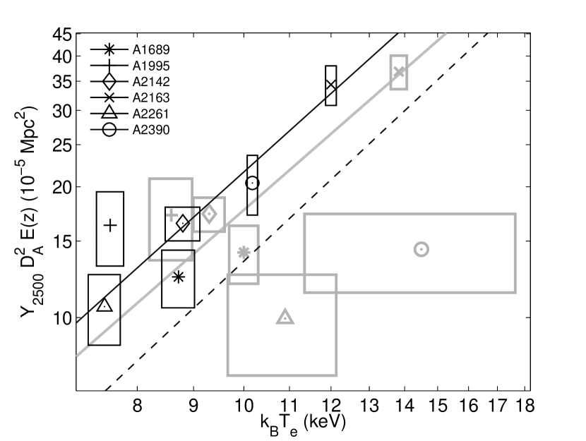
Figure 1.— The scaling relation between $Y_{2500}$ and $T_{\mathrm{e}}$. Those in solid black show the Chandra-based results. Those in gray show the ASCA/ROSAT-based results. Six clusters are labeled as indicated by the legend, with errors represented by the boxes. The lines are the best-fit power-law relations. The black dashed line is the best fit from Bonamente et al. (2008) for comparison.

4.2.2 The $Y_{2500}$ – $M_{2500}$ relation

The power-law index $B$ based on both sets of X-ray parameters are consistent with the self-similar model prediction of $B=1.67$. Our results also agree with the values of $B=1.66\pm 0.20$ from BIMA/OVRO (Bonamente et al., 2008), and $B=1.48\pm 0.39$ (CC+NCC sample) and $B=1.56\pm 0.29$ (CC only) from Morandi et al. (2007). Our normalization agrees with the value $A=-5.0\pm 3.0$ from BIMA/OVRO (Bonamente et al., 2008) and is consistent with the ranges $-5.09\lesssim A\lesssim-4.63$ (CC+NCC samples) and $-5.36\lesssim A\lesssim-4.91$ (CC only) given by Morandi et al. (2007). Here we convert the normalizations from other studies for comparison, such as $A=A^{\prime}+14B^{\prime}$ for BIMA/OVRO, and $A=A^{\prime}+\left(B^{\prime}-5/3\right)\log_{10}\overline{E(z)}-\log_{10}(10^{-8}I_{0})$ for Morandi et al. (2007), where $\overline{E(z)}$ is the mean $E(z)$ averaged over all AMiBA clusters.

Several analytical and numerical studies demonstrate that the integrated SZE signal, $Y_{2500}$ in our case, as a measure of the total pressure of inter-cluster medium is an excellent proxy for cluster total mass (da Silva et al., 2004; Motl et al., 2005; Nagai, 2006; Hallman et al., 2007). If this relationship could be measured to high precision at low redshifts, it could then be used to determine the masses of high-redshift SZE clusters and test cosmological models.

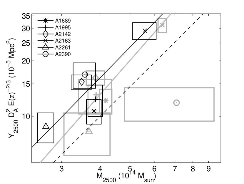
Figure 2.— The scaling relation between $Y_{2500}$ and $M_{2500}$. Symbols and colors are as defined in Fig. 1. The black dashed line refers to the best-fit from Bonamente et al. (2008) for comparison.

4.2.3 The $Y_{2500}$ – $L_{\mathrm{X}}$ relation

The power-law index for the $Y_{2500}-L_{\mathrm{X}}$ relation based on the Chandra set (after omitting A2142) is about $1.5\sigma$ lower than the theoretical value $B=1.25$, but is consistent with the results $B=0.81\pm 0.07$ (for CC+NCC sample) and $B=0.91\pm 0.11$ (for CC sample) given by Morandi et al. (2007). A low power-law index has also been observed in numerical simulations that include cooling or preheating processes (da Silva et al., 2004, $Y\propto L_{\mathrm{X}}$). The systematically lower power-law index relative to the self-similar model predication seems to imply that the relation between the SZE signals and X-ray luminosities is more sensitive to the radiative content outside 100 kpc than other scaling relations. However, none of the data points in Fig. 3 lies close to the best-fit line and the measure of goodness-of-fit, $\chi_{\mathrm{min}}^{2}/\mathrm{d.o.f.}$, is large (see Tab. 4). On the other hand, the normalization agrees with the result $-4.35\lesssim A\lesssim-4.01$ for CC+NCC sample within $1\sigma$ and is broadly consistent with $-4.47\lesssim A\lesssim-4.36$ for CC sample (Morandi et al., 2007), through the conversion of $A=A^{\prime}-(5/4-B^{\prime})\log_{10}\overline{E(z)}-\log_{10}\left(10^{-8}I_{0}\right)+B^{\prime}$.

The power-law index and normalization based on the ASCA/ROSAT set are consistent with the self-similar model. They also agree with the result based on the CC sample given by Morandi et al. (2007) within $1\sigma$, but only marginally consistent with those based on the CC+NCC sample. We observed, by comparing the values of different models in Allen (2000), that the additional component compensating the cooling flow emission in Model C will generally reduce the bolometric luminosities. If there is residual luminous emission, as Morandi et al. (2007) remarked that CC clusters systematically have larger luminosities than NCC ones even if the cooling cores have been handled, it would bias high the power (slope) and bias low the normalization (interception) shown in Fig. 3 in the sense of shifting the CC clusters to higher $L_{\mathrm{X}}$. This is a possible interpretation of the discrepancy for the CC+NCC sample, but again the scaling relation is not well defined, essentially by a scatter of CC cluster and a NCC cluster outside the scatter.

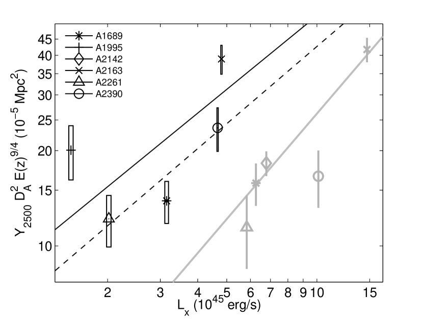
Figure 3.— The scaling relations between $Y_{2500}$ and $L_{\mathrm{X}}$. Symbols and colors are as defined in Fig. 1. The black dashed line shows the best-fit relation from Morandi et al. (2007) for comparison. The luminosities from the ASCA/ROSAT set are given without errors.

5. DISCUSSIONS

In the three figures of scaling relations we see that the Chandra-based relations are generally better fits than the ASCA/ROSAT-based relations, with smaller $\chi_{\mathrm{min}}^{2}$ and smaller errors on each data point. Although the $Y-L_{\mathrm{X}}$ relation based on the Chandra set has a larger scatter, there are no errors available for the luminosities of the ASCA/ROSAT set. Among clusters in the ASCA/ROSAT set, A2261 and A2390 have X-ray parameters of poor quality. A2390 seems to have a biased-high gas temperature or a systematically low $Y_{2500}$. A high temperature would lead to a high total mass based on the hydrostatic equilibrium equation, and would similarly increase the luminosity, which is related to the gas temperature as $L_{\mathrm{X}}\propto T_{\mathrm{e}}^{2}$ (Morandi et al., 2007).

Table 5Scaling relations $\log_{10}(y)=A+B\log_{10}(x)$ corrected for isothermal $\beta$-model

$x$	$y$	$A$	$B$	$\chi_{\mathrm{min}}^{2}$(d.o.f.)
$T_{\mathrm{e}}/keV$	$Y_{2500}D_{\mathrm{A}}^{2}E(z)/{\rm Mpc^{2}}$	$-6.16_{-0.74}^{+0.68}$	$2.31_{-0.70}^{+0.75}$	$1.74(4)$
$M_{2500}/10^{14}M_{\sun}$	$Y_{2500}D_{\mathrm{A}}^{2}E(z)^{-2/3}/{\rm Mpc^{2}}$	$-4.82_{-0.43}^{+0.30}$	$1.68_{-0.59}^{+0.87}$	$1.73(4)$
$L_{\mathrm{X}}/10^{45}{\rm erg\,s^{-1}}$	$Y_{2500}D_{\mathrm{A}}^{2}E(z)^{9/4}/{\rm Mpc^{2}}$	$-4.24_{-0.18}^{+0.18}$	$0.79_{-0.32}^{+0.32}$	$6.72(3)$

Note. — Errors are given at the $68.3\%$ confidence level.

Analytical and numerical studies reveal the fundamental incompatibility between $\beta$-model fits to X-ray surface brightness profiles and those done with SZE profiles (e.g.  Komatsu & Seljak, 2001; Hallman et al., 2007). Both X-ray and SZE fitted model parameters are biased due to the isothermal assumption, since the X-ray surface brightness and SZE Compton-$y$ parameter have different dependences on the cluster temperature profiles. This will generate an inconsistency in the model parameters based on isothermal $\beta$-model fits. Since observational SZE radial profiles are in short supply, X-ray driven parameters are often used to constrain the profile shape in SZE analysis, consequently leading to a bias in the derived values of cluster mass or Comptonization parameter.

To remedy this problem, we followed Hallman et al. (2007). Instead of re-fitting by the universal temperature profile proposed by Hallman et al. (2007), we simply modify our values of $\beta$, $r_{\mathrm{c}}$ and $Y_{2500}$ by the ratios between the values fitted from X-ray data on an isothermal $\beta$-model, and the ‘true’ values obtained from the simulation. We then re-calculate the scaling relations and these corrected results are summarized in Table 5. It is clear that the introduction of correction still keeps the scaling relations consistent with the uncorrected results, and the previous arguments and discussions are still valid. The scaling relations seem to be insensitive to this correction. As Hallman et al. (2007) discovered in their study of the $Y-M_{gas}$ relation, for example, the correlated changes in a $\beta$-model due to the definition of projected radius ($r_{2500}$ in our case) tend to cause compensating changes in the scaling relation.

We are aware that the entropy floor present in the cores of clusters could give rise to deviations from self-similar scalings (see e.g., McCarthy et al. (2003a, b)). X-ray observations have shown that scaling relations between several cluster observables deviate from the self-similar prediction, and it has been found that heating and cooling act in a similar manner by raising the mean entropy of the intracluster gas and, in some cases, establishing a core in the entropy profile. In McCarthy et al. (2003a) it was observed that the injection of excess entropy (preheating) will increase the temperature and reduce the gas pressure in the central regions of clusters, especially for the low-mass clusters. The scaling relations between the central value of the Compton-$y$ parameter, $y_{0}$, and the gas temperature or the total mass are most sensitive to the presence of excess entropy, and tend to develop larger power indices. Scaling relations involving the integrated Compton-$y$ parameter $Y$ show similar behaviors but are less sensitive, since the integration tends to reduce the effect of the entropy contribution from the cores.

6. CONCLUSIONS

In understanding cluster physics and cosmic evolution, the study of scaling relations for galaxy clusters is becoming more important since SZE observations such as those from the Sunyaev–Zel’dovich Array (SZA) and the South Pole Telescope (SPT) will detect clusters which are beyond X-ray detection limits, for which SZE scaling relations provide the first indications of cluster properties. In addition, deviations between the theoretical and observational results of the scaling relations can serve to examine the non-gravitational processes in the formation of clusters, which are not well understood at present.

As one of the few SZE instruments working at 3-mm, the AMiBA experiment observed six Abell clusters during 2007. The derived integrated Compton-$y$ parameters, $Y_{2500}$, are compared to other observations at different frequencies, as summarized in Table 3. Our results are consistent with those from BIMA/OVRO, but appear to show lower Comptonizations than those from SuZIE II. We have also investigated the three scaling relations between $Y_{2500}$ and the X-ray spectroscopic temperatures, total masses within $r_{2500}$, and bolometric X-ray luminosities. Our results for the scaling relations are summarized in Table 4.

Our power-law indices for the three scaling relations are broadly consistent with the self-similar model and observational results in the literature, except for that the $Y_{2500}-L_{\mathrm{X}}$ relation based on Chandra-derived parameters has a slope lower than the expectation of the self-similar model, and is sensitive to the chosen set of X-ray parameters and the treatment of cooling cores. These discrepancies might indicate either exotic properties for clusters or hidden flaws in our SZE data, although the scatter is still large, about a factor of two in the integrated Compton-$y$ relative to the fit line. The agreement between the normalizations found by different workers for our three scaling relations seems to support the idea that there is no strong scatter in the gas fraction (see Sec. 4.1).

In conclusion, the agreement between our results and those from the literature provides not only confidence for this project but also supports to our understanding of galaxy clusters. For AMiBA, significant improvements are expected following the expansion to a 13-element configuration with 1.2-m antennas (Ho et al., 2009, AMiBA13), which will provide better resolution and higher sensitivity. The capability of resolving SZE clusters will make it possible to measure the cluster profiles independent of the X-ray data (Molnar et al., 2009) and to estimate the properties of the clusters which currently do not have good X-ray data.

References

- Allen (2000) Allen, S. W. 2000, MNRAS, 315, 269
- Allen et al. (2001) Allen, S. W., Ettori, S., & Fabian, A. C. 2001, MNRAS, 324, 877
- Allen & Fabian (1998) Allen, S. W., & Fabian, A. C. 1998, MNRAS, 297, L57
- Benson et al. (2004) Benson, B., Ade, P., Bock, J., Ganga, K., Henson, C., Thompson, K., & Church, S. 2004, ApJ, 617, 829
- Böhringer et al. (1998) Böhringer, H., Tanaka, Y., Mushotzky, R. F., Ikebe, Y., & Hattori, M. 1998, A&A, 334, 789
- Bonamente et al. (2008) Bonamente, M., Joy, M., LaRoque, S. J., Carlstrom, J. E., Nagai, D., & Marrone, D. P. 2008, ApJ, 675, 106, 0708.0815
- Bonamente et al. (2006) Bonamente, M., Joy, M., Roque, S. L., Carlstrom, J., Reese, E., & Dawson, K. 2006, ApJ, 647, 25
- Cavaliere & Fusco-Femiano (1976) Cavaliere, A., & Fusco-Femiano, R. 1976, A&A, 49, 137
- Challinor & Lasenby (1998) Challinor, A. D., & Lasenby, A. N. 1998, ApJ, 499, 1
- Chen et al. (2009) Chen, M.-T. et al. 2009, ApJ, 694, 1664, 0902.3636
- da Silva et al. (2004) da Silva, A. C., Kay, S. T., Liddle, A. R., & Thomas, P. A. 2004, MNRAS, 348, 1401
- Grego et al. (2001) Grego, L., Carlstrom, J. E., Reese, E. D., Holder, G. P., Holzapfel, W. L., Joy, M. K., Mohr, J. J., & Patel, S. 2001, ApJ, 552, 2
- Hallman et al. (2007) Hallman, E. J., Burns, J. O., Motl, P. M., & Norman, M. L. 2007, ApJ, 665, 911
- Ho et al. (2009) Ho, P. T. P. et al. 2009, ApJ, 694, 1610, 0810.1871
- Kaiser (1986) Kaiser, N. 1986, MNRAS, 222, 323
- Koch et al. (2009a) Koch, P. M. et al. 2009a, ApJ, 694, 1670
- Koch et al. (2009b) ——. 2009b, ApJ, submitted
- Komatsu & Seljak (2001) Komatsu, E., & Seljak, U. 2001, MNRAS, 327, 1353
- Kravtsov et al. (2005) Kravtsov, A. V., Nagai, D., & Vikhlinin, A. A. 2005, ApJ, 625, 588
- Lancaster et al. (2005) Lancaster, K. et al. 2005, MNRAS, 359, 16, astro-ph/0405582
- LaRoque et al. (2006) LaRoque, S. J., Bonamente, M., Carlstrom, J. E., Joy, M. K., Nagai, D., Reese, E. D., & Dawson, K. S. 2006, ApJ, 652, 917
- Lin et al. (2009) Lin, K.-Y. et al. 2009, ApJ, 694, 1629, 0902.2437
- Liu et al. (2009) Liu, G.-C. et al. 2009, ApJ, submitted
- Markevitch et al. (2000) Markevitch, M. et al. 2000, ApJ, 541, 542
- Mather et al. (1999) Mather, J. C., Fixsen, D. J., Shafer, R. A., Mosier, C., & Wilkinson, D. T. 1999, ApJ, 512, 511
- McCarthy et al. (2002) McCarthy, I. G., Babul, A., & Balogh, M. L. 2002, ApJ, 573, 515
- McCarthy et al. (2003a) McCarthy, I. G., Babul, A., Holder, G. P., & Balogh, M. L. 2003a, ApJ, 591, 515
- McCarthy et al. (2003b) McCarthy, I. G., Holder, G. P., Babul, A., & Balogh, M. L. 2003b, ApJ, 591, 526
- Molnar et al. (2009) Molnar, S. M. et al. 2009, ApJ, submitted
- Morandi et al. (2007) Morandi, A., Ettori, S., & Moscardini, L. 2007, MNRAS, 379, 518, 0704.2678
- Motl et al. (2005) Motl, P. M., Hallman, E. J., Burns, J. O., & Norman, M. L. 2005, ApJ, 623, L63
- Mushotzky & Scharf (1997) Mushotzky, R. F., & Scharf, C. A. 1997, ApJ, 482, L13
- Myers et al. (1997) Myers, S. T., Baker, J. E., Readhead, A. C. S., Leitch, E. M., & Herbig, T. 1997, ApJ, 485, 1
- Nagai (2006) Nagai, D. 2006, ApJ, 650, 538
- Nagai et al. (2007) Nagai, D., Kravtsov, A. V., & Vikhlinin, A. 2007, ApJ, 668, 1, astro-ph/0703661
- Navarro et al. (1997) Navarro, J. F., Frenk, C. S., & White, S. D. M. 1997, ApJ, 490, 493
- Nishioka et al. (2009) Nishioka, H. et al. 2009, ApJ, 694, 1637, 0811.1675
- Patel et al. (2000) Patel, S. K. et al. 2000, ApJ, 541, 37
- Press et al. (2002) Press, W. H., Teukolsky, S. A., Vetterling, W. T., & Flannery, B. P. 2002, Numerical Recipes in C++. The Art of Scientific Computing, 2nd edn. (Cambridge University Press)
- Reese et al. (2002) Reese, E. D., Carlstrom, J. E., Joy, M., Mohr, J. J., Grego, L., & Holzapfel, W. L. 2002, ApJ, 581, 53
- Reiprich & Böhringer (2002) Reiprich, T. H., & Böhringer, H. 2002, ApJ, 567, 716
- Sanderson & Ponman (2003) Sanderson, A. J. R., & Ponman, T. J. 2003, MNRAS, 345, 1241
- Sunyaev & Zel’dovich (1970) Sunyaev, R. A., & Zel’dovich, Y. B. 1970, Comments Astrophys. Space Phys., 2, 66
- Udomprasert et al. (2004) Udomprasert, P. S., Mason, B. S., Readhead, A. C. S., & Pearson, T. J. 2004, ApJ, 615, 63
- Umetsu et al. (2009) Umetsu, K. et al. 2009, ApJ, 694, 1643, 0810.0969
- Vikhlinin (2006) Vikhlinin, A. 2006, ApJ, 640, 710
- Wu et al. (2009) Wu, J. H. P. et al. 2009, ApJ, 694, 1619, 0810.1015