Electromagnetic nature of dark energy

Abstract

Out of the four components of the electromagnetic field, Maxwell’s theory only contains two physical degrees of freedom. However, in an expanding universe, consistently eliminating one of the ”unphysical” states in the covariant (Gupta-Bleuler) formalism turns out to be difficult to realize. In this work we explore the possibility of quantization without subsidiary conditions. This implies that the theory would contain a third physical state. The presence of such a new (temporal) electromagnetic mode on cosmological scales is shown to generate an effective cosmological constant which can account for the accelerated expansion of the universe. This new polarization state is completely decoupled from charged matter, but can be excited gravitationally. In fact, primordial electromagnetic quantum fluctuations produced during electroweak scale inflation could naturally explain the presence of this mode and also the measured value of the cosmological constant. The theory is compatible with all the local gravity tests, it is free from classical or quantum instabilities and reduces to standard QED in the flat space-time limit. Thus we see that, not only the true nature of dark energy can be established without resorting to new physics, but also the value of the cosmological constant finds a natural explanation in the context of standard inflationary cosmology. Possible signals, discriminating this model from LCDM, are also discussed.

1 What is the nature of dark energy?

Although the standard cosmological constant provides a simple and accurate phenomenological description of the present phase of accelerated expansion of the universe acc , it is well known that it suffers from an important naturalness problem. Indeed, the scale of the cosmological constant around $10^{-3}$ eV is many orders of magnitude smaller than the fundamental gravity scale given by the Planck constant which is around $10^{19}$ GeV.

Alternative models based on new physics have been proposed, however they are generally plagued by:

• classical or quantum instabilities

• fine tuning problems

• inconsistencies with local gravity constraints

Also, the possibility that the accelerated expansion could be signaling the breakdown of General Relativity on large scales has been also proposed, and several modified gravity theories have been considered modified ; vector , although, in general, they also suffer from the same kind of problems described above.

However, apart from gravity there is another long-range interaction in nature which could be relevant on cosmological scales which is nothing but electromagnetism. It is usually assumed that due to the electric neutrality of the universe on large scales, the only relevant interaction in cosmology should be gravitation. However, the role played by electromagnetic astrophysical and cosmological fields is still far from clear, being the existence of cosmic magnetic fields the most evident example Grasso . As a matter of fact, and as for any other interaction in nature, electromagnetism has only been tested in a limited range of energies or distances, which are roughly below 1.3 A.U. Nieto and, as a consequence, no experimental evidence is available for electromagnetic fields whose wavelenghts are comparable to the present Hubble radius.

In this work, we consider (quantum) electromagnetic fields in an expanding universe. Unlike previous works, we will not follow the standard Coulomb gauge approach, but instead we will concentrate on the covariant quantization method. This method is found to exhibit certain difficulties when trying to impose the quantum Lorenz condition on cosmological scales Parker . In order to overcome these problems, and instead of introducing ghosts fields, we explore the possibility of quantizing without imposing any subsidiary condition EM ; sector . This implies that the electromagnetic field would contain an additional (scalar) polarization, similar to that generated in the massless limit of massive electrodynamics Deser . Interestingly, the energy density of quantum fluctuations of this new electromagnetic state generated during inflation gets frozen on cosmological scales, giving rise to an effective cosmological constant EM .

2 Electromagnetic quantization in flat space-time

Let us start by briefly reviewing electromagnetic quantization in Minkowski space-time Itzykson since this will be useful in the rest of the work. The action of the theory reads:

$$S=\int d^{4}x\left(-\frac{1}{4}F_{\mu\nu}F^{\mu\nu}+A_{\mu}J^{\mu}\right)$$ (1)

where $J_{\mu}$ is a conserved current. This action is invariant under gauge tranformations $A_{\mu}\rightarrow A_{\mu}+\partial_{\mu}\Lambda$ with $\Lambda$ an arbitrary function of space-time coordinates. At the classical level, this action gives rise to the well-known Maxwell’s equations:

$$\partial_{\nu}F^{\mu\nu}=J^{\mu}.$$ (2)

However, when trying to quantize the theory, several problems arise related to the redundancy in the description due to the gauge invariance. Thus, in particular, we find that it is not possible to construct a propagator for the $A_{\mu}$ field and also that ”unphysical” polarizations of the photon field are present. Two different approaches are usually followed in order to avoid these difficulties. In the first one, which is the basis of the Coulomb gauge quantization, the gauge invariance of the action (1) is used to eliminate the ”unphysical” degrees of freedom. With that purpose the (Lorenz) condition $\partial_{\mu}A^{\mu}=0$ is imposed by means of a suitable gauge transformation. Thus, the equations of motion reduce to:

$$\Box A_{\mu}=J_{\mu}.$$ (3)

The Lorenz condition does not fix completely the gauge freedom, still it is possible to perform residual gauge transformations $A_{\mu}\rightarrow A_{\mu}+\partial_{\mu}\theta$, provided $\Box\theta=0$. Using this residual symmetry and taking into account the form of equations (3), it is possible to eliminate one additional component of the $A_{\mu}$ field in the asymptotically free regions (typically $A_{0}$) which means $\vec{\nabla}\cdot\vec{A}=0$, so that finally the temporal and longitudinal photons are removed and we are left with the two transverse polarizations of the massless free photon, which are the only modes (with positive energies) which are quantized in this formalism.

The second approach is the basis of the covariant (Gupta-Bleuler) and path-integral formalisms. The starting point is a modification of the action in (1), namely:

$$S=\int d^{4}x\left(-\frac{1}{4}F_{\mu\nu}F^{\mu\nu}+\frac{\xi}{2}(\partial_{\mu}A^{\mu})^{2}+A_{\mu}J^{\mu}\right).$$ (4)

This action is no longer invariant under general gauge transformations, but only under residual ones. The equations of motion obtained from this action now read:

$$\partial_{\nu}F^{\mu\nu}+\xi\partial^{\mu}(\partial_{\nu}A^{\nu})=J^{\mu}.$$ (5)

In order to recover Maxwell’s equation, the Lorenz condition must be imposed so that the $\xi$ term disappears. At the classical level this can be achieved by means of appropriate boundary conditions on the field. Indeed, taking the four-divergence of the above equation, we find:

$$\Box(\partial_{\nu}A^{\nu})=0$$ (6)

where we have made use of current conservation. This means that the field $\partial_{\nu}A^{\nu}$ evolves as a free scalar field, so that if it vanishes for large $|t|$, it will vanish at all times. At the quantum level, the Lorenz condition cannot be imposed as an operator identity, but only in the weak sense $\partial_{\nu}A^{\nu\,(+)}|\phi\rangle=0$, where $(+)$ denotes the positive frequency part of the operator and $|\phi\rangle$ is a physical state. This condition is equivalent to imposing $[{\bf a}_{0}(\vec{k})+{\bf a}_{\parallel}(\vec{k})]|\phi\rangle=0$, with ${\bf a}_{0}$ and ${\bf a}_{\parallel}$ the annihilation operators corresponding to temporal and longitudinal electromagnetic states. Thus, in the covariant formalism, the physical states contain the same number of temporal and longitudinal photons, so that their energy densities, having opposite signs, cancel each other.

Thus we see that also in this case, the Lorenz condition seems to be essential in order to recover standard Maxwell’s equations and get rid of the negative energy states.

3 Covariant quantization in an expanding universe

So far we have only considered Maxwell’s theory in flat space-time, however when we move to a curved background, and in particular to an expanding universe, then consistently imposing the Lorenz condition in the covariant formalism turns out to be difficult to realize. Indeed, let us consider the curved space-time version of action (4):

$$S=\int d^{4}x\sqrt{g}\left[-\frac{1}{4}F_{\mu\nu}F^{\mu\nu}+\frac{\xi}{2}(\nabla_{\mu}A^{\mu})^{2}+A_{\mu}J^{\mu}\right]$$ (7)

Now the modified Maxwell’s equations read:

$$\nabla_{\nu}F^{\mu\nu}+\xi\nabla^{\mu}(\nabla_{\nu}A^{\nu})=J^{\mu}$$ (8)

and taking again the four divergence, we get:

$$\Box(\nabla_{\nu}A^{\nu})=0$$ (9)

We see that once again $\nabla_{\nu}A^{\nu}$ behaves as a scalar field which is decoupled from the conserved electromagnetic currents, but it is non-conformally coupled to gravity. This means that, unlike the flat space-time case, this field can be excited from quantum vacuum fluctuations by the expanding background in a completely analogous way to the inflaton fluctuations during inflation. Thus this poses the question of the validity of the Lorenz condition at all times.

In order to illustrate this effect, we will present a toy example. Let us consider quantization in the absence of currents, in a spatially flat expanding background, whose metric is written in conformal time as $ds^{2}=a(\eta)^{2}(d\eta^{2}-d\vec{x}^{2})$ with $a(\eta)=2+\tanh(\eta/\eta_{0})$ where $\eta_{0}$ is constant. This metric possesses two asymptotically Minkowskian regions in the remote past and far future. We solve the coupled system of equations (8) for the corresponding Fourier modes, which are defined as ${\mathcal{A}}_{\mu}(\eta,\vec{x})=\int d^{3}k{\mathcal{A}}_{\mu\vec{k}}(\eta)e^{i\vec{k}\vec{x}}$. Thus, for a given mode $\vec{k}$, the ${\mathcal{A}}_{\mu}$ field is decomposed into temporal, longitudinal and transverse components. The corresponding equations read:

$${\mathcal{A}}_{0k}^{\prime\prime} - \left[\frac{k^{2}}{\xi}-2{\mathcal{H}}^{\prime}+4{\mathcal{H}}^{2}\right]{\mathcal{A}}_{0k}-2ik\left[\frac{1+\xi}{2\xi}{\mathcal{A}}_{\parallel k}^{\prime}-{\mathcal{H}}{\mathcal{A}}_{\parallel k}\right]=0$$

$${\mathcal{A}}_{\parallel k}^{\prime\prime} - k^{2}\xi{\mathcal{A}}_{\parallel k}-2ik\xi\left[\frac{1+\xi}{2\xi}{\mathcal{A}}_{0k}^{\prime}+{\mathcal{H}}{\mathcal{A}}_{0k}\right]=0$$

$$\vec{{\mathcal{A}}}_{\perp k}^{\prime\prime} + k^{2}\vec{{\mathcal{A}}}_{\perp k}=0$$ (10)

with ${\cal H}=a^{\prime}/a$ and $k=|\vec{k}|$. We see that the transverse modes are decoupled from the background, whereas the temporal and longitudinal ones are non-trivially coupled to each other and to gravity. Let us prepare our system in an initial state $|\phi\rangle$ belonging to the physical Hilbert space, i.e. satisfying $\partial_{\nu}{\mathcal{A}}^{\nu\,(+)}_{in}|\phi\rangle=0$ in the initial flat region. Because of the expansion of the universe, the positive frequency modes in the $in$ region with a given temporal or longitudinal polarization $\lambda$ will become a linear superposition of positive and negative frequency modes in the $out$ region and with different polarizations $\lambda^{\prime}$ (in this section we will work in the Feynman gauge $\xi=-1$), thus we have:

$${\mathcal{A}}_{\mu\vec{k}}^{\lambda\;(in)}=\sum_{\lambda^{\prime}=0,\parallel}\left[\alpha_{\lambda\lambda^{\prime}}(\vec{k}){\mathcal{A}}_{\mu\,\vec{k}}^{\lambda^{\prime}\;(out)}+\beta_{\lambda\lambda^{\prime}}(\vec{k})\overline{{\mathcal{A}}_{\mu\,-\vec{k}}^{\lambda^{\prime}\;(out)}}\,\right]$$ (11)

or in terms of creation and annihilation operators:

$${\bf a}_{\lambda^{\prime}}^{(out)}(\vec{k})=\sum_{\lambda=0,\parallel}\left[\alpha_{\lambda\lambda^{\prime}}(\vec{k}){\bf a}_{\lambda}^{(in)}(\vec{k})+\overline{\beta_{\lambda\lambda^{\prime}}(\vec{k})}{\bf a}_{\lambda}^{(in)\dagger}(-\vec{k})\right]$$ (12)

with $\lambda,\lambda^{\prime}=0,\parallel$ and where $\alpha_{\lambda\lambda^{\prime}}$ and $\beta_{\lambda\lambda^{\prime}}$ are the so-called Bogolyubov coefficients (see Birrell for a detailed discussion), which are normalized in our case according to:

$$\sum_{\rho,\rho^{\prime}=0,\parallel}(\alpha_{\lambda\rho}\,\overline{\alpha_{\lambda^{\prime}\rho^{\prime}}}\,\eta_{\rho\rho^{\prime}}-\beta_{\lambda\rho}\,\overline{\beta_{\lambda^{\prime}\rho^{\prime}}}\,\eta_{\rho\rho^{\prime}})=\eta_{\lambda\lambda^{\prime}}$$ (13)

with $\eta_{\lambda\lambda^{\prime}}=diag(-1,1)$ with $\lambda,\lambda^{\prime}=0,\parallel$. Notice that the normalization is different from the standard one Birrell , because of the presence of negative norm states.

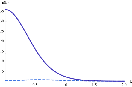
Figure 1: Occupation numbers for temporal (continuous line) and longitudinal (dashed line) photons in the $out$ region vs. $k$ in $\eta_{0}^{-1}$ units.

Thus, the system will end up in a final state which no longer satisfies the weak Lorenz condition i.e. in the out region $\partial_{\nu}{\mathcal{A}}^{\nu\,(+)}_{out}|\phi\rangle\neq 0$. This is shown in Fig. 1, where we have computed the final number of temporal and longitudinal photons $n_{\lambda^{\prime}}^{out}(k)=\sum_{\lambda}|\beta_{\lambda\lambda^{\prime}}(\vec{k})|^{2}$, starting from an initial vacuum state with $n_{0}^{in}(k)=n_{\parallel}^{in}(k)=0$. We see that, as commented above, in the final region $n_{0}^{out}(k)\neq n_{\parallel}^{out}(k)$ and the state no longer satisfies the Lorenz condition. Notice that the failure comes essentially from large scales, i.e. super-Hubble scales with $k\eta_{0}\ll 1$, since on small (sub-Hubble) scales with $k\eta_{0}\gg 1$, the Lorenz condition is restored. This can be easily interpreted from the fact that on small scales the geometry can be considered as essentially Minkowskian.

In order to overcome this problem, it is possible to impose a more stringent gauge-fixing condition. Indeed, we have shown above that in a space-time configuration with asymptotic flat regions, an initial state satisfying the weak Lorenz condition does not necessarily satisfy it at a later time. However, it would be possible (see Pfenning ) to define the physical states $|\phi\rangle$ as those such that $\nabla_{\mu}A^{\mu(+)}|\phi\rangle=0$, $\forall\eta$. Although this is a perfectly consistent solution, notice that the separation in positive and negative frequency parts depends on the space-time geometry and therefore, the determination of the physical states requires a previous knowledge of the future evolution of the universe.

Another possible way out would be to modify the standard Gupta-Bleuler formalism by including ghosts fields as done in non-abelian gauge theories Kugo . With that purpose, the action of the theory (7) can be modified by including the ghost term (see Adler ):

$$S_{g}=\int d^{4}x\sqrt{g}\,g^{\mu\nu}\,\partial_{\mu}\bar{c}\,\partial_{\nu}c$$ (14)

where $c$ are the complex scalar ghost fields. It is a well-known result Adler ; BO that by choosing appropriate boundary conditions for the electromagnetic and ghosts Green’s functions, it is possible to get $\langle\phi|T_{\mu\nu}^{\xi}+T_{\mu\nu}^{g}|\phi\rangle=0$, where $T_{\mu\nu}^{\xi}$ and $T_{\mu\nu}^{g}$ denote the contribution to the energy-momentum tensor from the $\xi$ term in (7) and from the ghost term (14) respectively. Notice that a choice of boundary conditions in the Green’s functions corresponds to a choice of vacuum state. Therefore, also in this case an a priori knowledge of the future behaviour of the universe expansion is required in order to determine the physical states.

Although these are valid quanization procedures, in this work we follow a different approach in order to deal with the difficulties found in the Gupta-Bleuler formalism and we will explore the possibility of quantization in an expanding universe without imposing any subsidiary condition.

4 Quantization without the Lorenz condition

In the previous section it has been shown that although the Lorenz gauge-fixing conditions can be formally imposed in the covariant formalism, this cannot be done in a straightforward way. These difficulties could be suggesting some more fundamental obstacle in the formulation of an electromagnetic gauge invariant theory in an expanding universe. As a matter of fact, electromagnetic models which break gauge invariance on cosmological scales have been widely considered in the context of generation of primordial magnetic fields (see, for instance, Turner ).

Let us then explore the possibility that the fundamental theory of electromagentism is not given by the gauge invariant action (1), but by the gauge non-invariant action (7). Abandoning gauge invariance could, in principle, pose important problems for the viability of the theory, namely:

• Modification of classical Maxwell’s equations

• Electric charge non-conservation

• New unobserved photon polarizations

• Negative norm (energy) states

• Conflicts with QED phenomenology

However, as we will show in the following, none of these problems is actually present for the theory in (7).

Since the fundamental electromagnetic theory is assumed to be non-invariant under arbitrary gauge transformations, then there is no need to impose the Lorenz constraint in the quantization procedure. Therefore, having removed one constraint, the theory contains one additional degree of freedom. Thus, the general solution for the modified equations (8) can be written as:

$${\mathcal{A}}_{\mu}={\mathcal{A}}_{\mu}^{(1)}+{\mathcal{A}}_{\mu}^{(2)}+{\mathcal{A}}_{\mu}^{(s)}+\partial_{\mu}\theta$$ (15)

where ${\mathcal{A}}_{\mu}^{(i)}$ with $i=1,2$ are the two transverse modes of the massless photon, ${\mathcal{A}}_{\mu}^{(s)}$ is the new scalar state, which is the mode that would have been eliminated if we had imposed the Lorenz condition and, finally, $\partial_{\mu}\theta$ is a purely residual gauge mode, which can be eliminated by means of a residual gauge transformation in the asymptotically free regions, in a completely analogous way to the elimination of the $A_{0}$ component in the Coulomb quantization. The fact that Maxwell’s electromagnetism could contain an additional scalar mode decoupled from electromagnetic currents, but with non-vanishing gravitational interactions, was already noticed in a different context in Deser .

In order to quantize the free theory, we perform the mode expansion of the field with the corresponding creation and annihilation operators for the three physical states:

$${\mathcal{A}}_{\mu}=\int d^{3}\vec{k}\ \sum_{\lambda=1,2,s}\left[{\bf a}_{\lambda}(k){\mathcal{A}}_{\mu k}^{(\lambda)}+{\bf a}_{\lambda}^{\dagger}(k)\overline{{\mathcal{A}}_{\mu k}^{(\lambda)}}\,\right]$$ (16)

where the modes are required to be orthonormal with respect to the scalar product (see for instance Pfenning ):

$$\left({\mathcal{A}}^{(\lambda)}_{k},{\mathcal{A}}^{(\lambda^{\prime})}_{k^{\prime}}\right) = i\int_{\Sigma}d\Sigma_{\mu}\left[\,\overline{{\mathcal{A}}_{\nu k}^{(\lambda)}}\;\Pi^{(\lambda^{\prime})\mu\nu}_{k^{\prime}}-\overline{\Pi^{(\lambda)\mu\nu}_{k}}\;{\mathcal{A}}_{\nu k^{\prime}}^{(\lambda^{\prime})}\right]$$ (17)

$$= \delta_{\lambda\lambda^{\prime}}\delta^{(3)}(\vec{k}-\vec{k}^{\prime}),\;\;\;\;\;\lambda,\lambda^{\prime}=1,2,s$$

where $d\Sigma_{\mu}$ is the three-volume element of the Cauchy hypersurfaces. In a Robertson-Walker metric in conformal time, it reads $d\Sigma_{\mu}=a^{4}(\eta)(d^{3}x,0,0,0)$. The generalized conjugate momenta are defined as:

$$\Pi^{\mu\nu}=-(F^{\mu\nu}-\xi g^{\mu\nu}\nabla_{\rho}A^{\rho})$$ (18)

Notice that the three modes can be chosen to have positive normalization. The equal-time commutation relations:

$$\left[{\mathcal{A}}_{\mu}(\eta,\vec{x}),{\mathcal{A}}_{\nu}(\eta,\vec{x}\,^{\prime})\right]=\left[\Pi^{0\mu}(\eta,\vec{x}),\Pi^{0\nu}(\eta,\vec{x},^{\prime})\right]=0$$ (19)

and

$$\left[{\mathcal{A}}_{\mu}(\eta,\vec{x}),\Pi^{0\nu}(\eta,\vec{x}\,^{\prime})\right]=i\frac{\delta_{\mu}^{\;\nu}}{\sqrt{g}}\delta^{(3)}(\vec{x}-\vec{x}\,^{\prime})$$ (20)

can be seen to imply the canonical commutation relations:

$$\left[{\bf a}_{\lambda}(\vec{k}),{\bf a}_{\lambda^{\prime}}^{\dagger}(\vec{k^{\prime}})\right]=\delta_{\lambda\lambda^{\prime}}\delta^{(3)}(\vec{k}-\vec{k^{\prime}}),\;\;\;\lambda,\lambda^{\prime}=1,2,s$$ (21)

by means of the normalization condition in (17). Notice that the sign of the commutators is positive for the three physical states, i.e. there are no negative norm states in the theory, which in turn implies that there are no negative energy states as we will see below in an explicit example.

Since $\nabla_{\mu}{\mathcal{A}}^{\mu}$ evolves as a minimally coupled scalar field, as shown in (9), on sub-Hubble scales ($|k\eta|\gg 1$), we find that for arbitrary background evolution, $|\nabla_{\mu}{\mathcal{A}}^{(s)\mu}_{k}|\propto a^{-1}$, i.e. the field is suppressed by the universe expansion, thus effectively recovering the Lorenz condition on small scales. Notice that this is a consequence of the cosmological evolution, not being imposed as a boundary condition as in the flat space-time case.

On the other hand, on super-Hubble scales ($|k\eta|\ll 1$), $|\nabla_{\mu}{\mathcal{A}}^{(s)\mu}_{k}|=const.$ which, as shown in EM , implies that the field contributes as a cosmological constant in (7). Indeed, the energy-momentum tensor derived from (7) reads:

$$T_{\mu\nu} = -F_{\mu\alpha}F_{\nu}^{\;\;\alpha}+\frac{1}{4}g_{\mu\nu}F_{\alpha\beta}F^{\alpha\beta}$$ (22)

$$+ \frac{\xi}{2}\left[g_{\mu\nu}\left[\left(\nabla_{\alpha}A^{\alpha}\right)^{2}+2A^{\alpha}\nabla_{\alpha}\left(\nabla_{\beta}A^{\beta}\right)\right]-4A_{(\mu}\nabla_{\nu)}\left(\nabla_{\alpha}A^{\alpha}\right)\right]$$

Notice that, for the scalar electromagnetic mode in the super-Hubble limit, the contributions involving $F_{\mu\nu}$ vanish and only the piece proportional to $\xi$ is relevant. Thus, it can be easily seen that, since in this case $\nabla_{\alpha}A^{\alpha}=constant$, the energy-momentum tensor is just given by:

$$T_{\mu\nu}=\frac{\xi}{2}g_{\mu\nu}(\nabla_{\alpha}A^{\alpha})^{2}$$ (23)

which is the energy-momentum tensor of a cosmological constant. Notice that, as seen in (9), the new scalar mode is a massless free field. This is one of the most relevant aspects of the present model in which, unlike existing dark energy theories based on scalar fields, dark energy can be generated without including any potential term or dimensional constant.

Since, as shown above, the field amplitude remains frozen on super-Hubble scales and starts decaying once the mode enters the horizon in the radiation or matter eras, the effect of the $\xi$ term in (8) is completely negligible on sub-Hubble scales, since the initial amplitude generated during inflation is very small as we will show below. Thus, below 1.3 AU, which is the largest distance scale at which electromagnetism has been tested Nieto , the modified Maxwell’s equations (8) are physically indistinguishable from the flat space-time ones (2).

Notice that in Minkowski space-time, the theory (7) is completely equivalent to standard QED. This is so because, although non-gauge invariant, the corresponding effective action is equivalent to the standard BRS invariant effective action of QED. Thus, the effective action for QED obtained from (2) by the standard gauge-fixing procedure reads:

$$e^{iW}=\int[dA][dc][d\bar{c}][d\psi][d\bar{\psi}]e^{i\int d^{4}x\left(-\frac{1}{4}F_{\mu\nu}F^{\mu\nu}+\frac{\xi}{2}(\partial_{\mu}A^{\mu})^{2}+\eta^{\mu\nu}\partial_{\mu}\bar{c}\,\partial_{\nu}c+{\cal L}_{F}\right)}$$ (24)

where ${\cal L}_{F}$ is the Lagrangian density of charged fermions. The $\xi$ term and the ghosts field appear in the Faddeev-Popov procedure when selecting an element of each gauge orbit. However, ghosts being decoupled from the electromagnetic currents can be integrated out in flat space-time, so that up to an irrelevant normalization constant we find:

$$e^{iW}=\int[dA][d\psi][d\bar{\psi}]e^{i\int d^{4}x\left(-\frac{1}{4}F_{\mu\nu}F^{\mu\nu}+\frac{\xi}{2}(\partial_{\mu}A^{\mu})^{2}+{\cal L}_{F}\right)}$$ (25)

which is nothing but the effective action coming from the gauge non-invariant theory (7) in flat space-time, in which no gauge-fixing procedure is required.

To summarize, none of the above mentioned consistency problems for the theory in (7) arise, thus:

• Ordinary Maxwell’s equations are recovered on those small scales in which electromagnetism has been tested.

• Electric charge is conserved since only the gauge electromagnetic sector is modified but not the sector of charged particles which preserves its gauge symmetry.

• The new state only couples gravitationally and evades laboratory detection.

• The new state has positive norm (energy).

• The effective action is completely equivalent to standard QED in the flat space-time limit. This guarantees, not only that the standard phenomenology is recovered, but also that no new interaction terms will appear in the renormalization procedure.

5 Cosmological evolution

Let us now consider the cosmological evolution of this new electromagnetic mode. For that purpose, we will consider an homogeneous electromagnetic field with $A_{\mu}=(A_{0}(t),\vec{A}(t))$. The corresponding equations motion in a flat Robertson-Walker background in cosmological time $t$ read:

$$\ddot{A}_{0} + 3H\dot{A}_{0}+3\dot{H}A_{0}=0$$

$$\ddot{\vec{A}} + H\dot{\vec{A}}=0$$ (26)

Notice that conformal time components are related to components in cosmological time as ${\mathcal{A}}_{\mu}=(aA_{0},\vec{A})$. The effects of the high electric conductivity of the universe can be taken into account by including the corresponding current term $J^{\mu}$ on the right hand side of Maxwell’s equations, however due to the strict electric neutrality of the universe on large scales $J^{\mu}=0$.

In the case in which the scale factor behaves as a simple power law with $H=p/t$, the solutions for the above equations are:

$$A_{0}(t) = A_{0}^{+}t+A_{0}^{-}t^{-3p}$$

$$\vec{A}(t) = \vec{A}^{+}t^{1-p}+\vec{A}^{-}$$ (27)

Thus we see that the temporal component grows faster than the spatial one and therefore, at late times, on cosmological scales we can ignore the spatial contribution and the new scalar state is essentially given by the electric potential. Notice also that from the temporal equation we get:

$$\frac{d}{dt}(\nabla_{\mu}A^{\mu})=\frac{d}{dt}(\dot{A}_{0}+3HA_{0})=0$$ (28)

irrespective of the background evolution, i.e. on large scales the scalar mode $\nabla_{\mu}A^{\mu}$ is strictly constant as commented before. We can also compute the contributions from the temporal and spatial components to the energy density from (22), thus we get:

$$\rho_{A_{0}} = \frac{\lambda}{2}\left(\dot{A}_{0}+3HA_{0}\right)^{2}=\,const.$$

$$\rho_{\vec{A}} = \frac{1}{2a^{2}}\left(\dot{\vec{A}}\right)^{2}\propto\,a^{-4}$$ (29)

We see that also, as commented before, the temporal component behaves as a cosmological constant, whereas the contibution from the spatial part decays as radiation and therefore does not affect the universe isotropy on large scales.

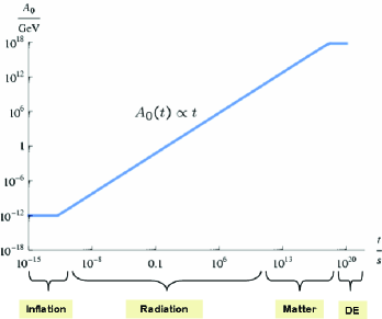
Figure 2: Cosmological evolution of the temporal component from electroweak-scale inflation until present

In Fig.2 we show the cosmological evolution of the electric potential $A_{0}$. We see that the field is constant during inflation, it grows linearly in time in the matter and radiation eras and becomes also constant when the eletromagnetic dark energy starts dominating. Notice that the present value of $A_{0}$ will be determined by the initial value of the field generated during inflation from quantum fluctuations. This amplitude can be explicitly calculated as shown in next section.

6 Quantum fluctuations during inflation

Let us consider the quantization in an inflationary de Sitter space-time with $a(\eta)=-1/(H_{I}\eta)$. Here we will take $\xi=1/3$, although similar results can be obtained for any $\xi>0$. The explicit solution for the normalized scalar state is EM :

$${\mathcal{A}}_{0k}^{(s)} = -\frac{1}{(2\pi)^{3/2}}\frac{i}{\sqrt{2k}}\left\{k\eta e^{-ik\eta}\right.$$

$$+ \left.\frac{1}{k\eta}\left[\frac{1}{2}(1+ik\eta)e^{-ik\eta}-k^{2}\eta^{2}e^{ik\eta}E_{1}(2ik\eta)\right]\right\}e^{i\vec{k}\vec{x}}$$

$${\mathcal{A}}_{\parallel k}^{(s)} = \frac{1}{(2\pi)^{3/2}}\frac{1}{\sqrt{2k}}\left\{(1+ik\eta)e^{-ik\eta}\right.$$ (30)

$$- \left.\left[\frac{3}{2}e^{-ik\eta}+(1-ik\eta)e^{ik\eta}E_{1}(2ik\eta)\right]\right\}e^{i\vec{k}\vec{x}}$$

where $E_{1}(x)=\int_{1}^{\infty}e^{-tx}/tdt$ is the exponential integral function. Using this solution, we find:

$$\nabla_{\mu}{\mathcal{A}}^{(s)\mu}_{k}=-\frac{a^{-2}(\eta)}{(2\pi)^{3/2}}\frac{ik}{\sqrt{2k}}\frac{3}{2}\frac{(1+ik\eta)}{k^{2}\eta^{2}}e^{-ik\eta+i\vec{k}\vec{x}}$$ (31)

so that the field is suppressed in the sub-Hubble limit as $\nabla_{\mu}{\mathcal{A}}^{(s)\mu}_{k}\sim{\cal O}((k\eta)^{-2})$.

On the other hand, from the energy density given by $\rho_{A}=T^{0}_{\;\;0}$, we obtain in the sub-Hubble limit the corresponding Hamiltonian, which is given by:

$$H=\frac{1}{2}\int\frac{d^{3}\vec{k}}{a^{4}(\eta)}k\sum_{\lambda=1,2,s}\left[{\bf a}_{\lambda}^{\dagger}(\vec{k}){\bf a}_{\lambda}(\vec{k})+{\bf a}_{\lambda}(\vec{k}){\bf a}_{\lambda}^{\dagger}(\vec{k})\right].$$ (32)

We see that the theory does not contain negative energy states (ghosts).

Finally, from (30) it is possible to obtain the dispersion of the effective cosmological constant during inflation:

$$\langle 0|(\nabla_{\mu}{\mathcal{A}}^{\mu})^{2}|0\rangle=\int\frac{dk}{k}P_{A}(k)$$ (33)

with $P_{A}(k)=4\pi k^{3}|\nabla_{\mu}{\mathcal{A}}^{(s)\mu}_{k}|^{2}$. In the super-Hubble limit, we obtain for the power-spectrum:

$$P_{A}(k)=\frac{9H_{I}^{4}}{16\pi^{2}},$$ (34)

in agreement with EM . Notice that this result implies that $\rho_{A}\sim(H_{I})^{4}$. The measured value of the cosmological constant then requires $H_{I}\sim 10^{-3}$ eV, which corresponds to an inflationary scale $M_{I}\sim 1$ TeV. Thus we see that the cosmological constant scale can be naturally explained in terms of physics at the electroweak scale.

7 Perturbations and consistency

Despite the fact that the background evolution in the present case is the same as in $\Lambda$CDM, the evolution of metric perturbations could be different, thus offering an observational way of discriminating between the two models. With this purpose, we have calculated the evolution of metric, matter density and electromagnetic perturbations BKMM . The propagation speeds of scalar, vector and tensor perturbations are found to be real and equal to the speed of light, so that the theory is classically stable. We have also shown before that the theory does not contain ghosts and it is therefore stable at the quantum level. On the other hand, using the explicit expressions in Will for the vector-tensor theory of gravity corresponding to the action in (7), it is possible to see that all the parametrized post-Newtonian (PPN) parameters agree with those of General Relativity, i.e. the theory is compatible with all the local gravity constraints for any value of the homogeneous background electromagnetic field EM ; VT .

Concerning the evolution of scalar perturbations, we find that the only relevant deviations with respect to $\Lambda$CDM appear on large scales $k\sim H_{0}$ and that they depend on the primordial spectrum of electromagnetic fluctuations. However, the effects on the CMB temperature and matter power spectra are compatible with observations except for very large primordial fluctuations. In addition, the different evolution of the scalar potential $\Phi_{k}$ with respect to the $\Lambda$CDM model gives rise to a possible discriminating contribution to the late-time integrated Sachs-Wolfe effect Turok .

8 Conclusions

In this work we have presented a consistent quantization procedure for the electromagnetic interaction with three polarization states. The energy density of the new scalar mode on cosmological scales is shown to behave as an effective cosmological constant, whose value is determined by the amplitude of quantum fluctuations generated during inflation. As a matter of fact, the measured value of the cosmological constant is naturally explained provided inflation took place at the electroweak scale. The model is free from classical or quantum instablities and is consistent with all the local gravity constraints. On the other hand, it is also compatible with observations from CMB and large scale structure and contains the same number of free parameters as $\Lambda$CDM. Unlike dark energy models based on scalar fields, acceleration in this model arises from the kinetic term of the new electromagnetic mode, without the introduction of unnatural dimensional parameters or potential terms. The results presented in this work show that, unlike previous proposals, the nature of dark energy can be established without resorting to new physics.

Acknowledgments: This work has been supported by Ministerio de Ciencia e Innovación (Spain) project numbers FIS 2008-01323 and FPA 2008-00592, UCM-Santander PR34/07-15875, CAM/UCM 910309 and MEC grant BES-2006-12059.

References

- (1) S. Perlmutter et al., Astrophys. J. 517, 565 (1999); A.G. Riess et al., Astron. J. 116, 1009 (1998) and 117, 707 (1999); D. N. Spergel et al. Astrophys. J. Suppl. 148, 175, (2003) and astro-ph/0603449; M. Tegmark et al., Phys. Rev. D69: 103501, (2004).
- (2) S.M. Carroll, V. Duvvuri, M. Trodden, M.S. Turner, Phys. Rev. D70: 043528, (2004); G. Dvali, G. Gabadadze and M. Porrati, Phys. Lett. B485, 208 (2000).
- (3) V.V. Kiselev, Class. Quant. Grav. 21: 3323, (2004); C. Armendariz-Picon, JCAP 0407: 007, (2004); J. Beltrán Jiménez and A.L. Maroto, Phys. Rev. D78, 063005 (2008) and arXiv:0807.2528 [astro-ph]; T. Koivisto and D.F. Mota, JCAP 0808: 021 (2008); K. Bamba, S. Nojiri and S.D. Odintsov, Phys. Rev. D77, 123532 (2008).
- (4) D. Grasso and H. R. Rubinstein, Phys. Rept. 348 163 (2001).
- (5) A.S. Goldhaber and M.M. Nieto, arXiv:0809.1003 [hep-ph].
- (6) A. Higuchi, L. Parker and Y. Wang, Phys. Rev. D 42, 4078 (1990).
- (7) J. Beltrán Jiménez and A.L. Maroto, JCAP 0903: 016 (2009), arXiv:0811.0566 and arXiv:0905.2589 to appear in Int. J. Mod. Phys. D.
- (8) J. Beltrán Jiménez and A.L. Maroto, arXiv:0903.4672
- (9) S. Deser, Ann. Inst. Henri Poincaré, 16: 79 (1972)
- (10) C. Itzykson and J.B. Zuber, Quantum Field Theory, McGraw-Hill (1980); N.N. Bogoliubov and D.V. Shirkov, Introduction to the theory of quantized fields, Interscience Publishers, Inc. (1959).
- (11) N.D. Birrell and P.C.W. Davies, Quantum fields in curved space, Cambridge (1982).
- (12) M. J. Pfenning, Phys. Rev. D65 024009 (2002).
- (13) T. Kugo and I. Ojima, Phys. Lett. B 73 (1978) 459.
- (14) S. L. Adler, J. Lieberman and Y. J. Ng, Annals Phys. 106, 279 (1977); B.S. DeWitt and R.W. Brehme, Annals Phys. 9, 220 (1960)
- (15) M. R. Brown and A. C. Ottewill, Phys. Rev. D 34, 1776 (1986).
- (16) Michael S. Turner and Lawrence M. Widrow, Phys. Rev. D37: 2743, (1988)
- (17) J. B. Jimenez, T. S. Koivisto, A. L. Maroto and D. F. Mota, JCAP 0910: 029 (2009), arXiv:0907.3648.
- (18) C. Will, Theory and experiment in gravitational physics, Cambridge University Press, (1993)
- (19) J. Beltrán Jiménez and A.L. Maroto, JCAP 0902: 025 (2009), e-Print: arXiv:0811.0784 [astro-ph] and AIP Conf.Proc.1122:107-114, (2009), arXiv:0812.1970.
- (20) R.G. Crittenden and N. Turok, Phys. Rev. Lett. 76 (1996) 575