Correlated-Photon Imaging with Cancellation of Object-Induced Aberration

Abstract

We show that a recently discussed apparatus for aberration-cancelled interferometry may be modified to perform correlated-photon imaging in the so-called ”ghost” imaging configuration. For objects in the vicinity of a particular plane, the images are free of object-induced phase distortions. This apparatus has the distinctive feature that it may be used to superimpose images of two objects in a manner that could lead to useful effects and applications. We show that the apparatus works using either quantum-entangled or classically correlated light sources.

I INTRODUCTION

Correlated-photon imaging, sometimes known as ”ghost” imaging, was first discovered using entangled photon pairs pittman (1) from spontaneous parametric downconversion (SPDC). It has since been found that most aspects of ghost imaging can be simulated using spatially-correlated classical light bennink1 (2, 3), including thermal and speckle sources gatti (4, 5, 6, 7, 8, 9). A separate line of research has shown that entangled photon pairs from downconversion may also be used to cancel some of the effects of frequency dispersion steinberg (11, 10, 12) or spatial dispersion (aberration) bonato1 (13, 14, 15). In simon1 (15), it was pointed out that it is possible to construct an interferometer such that if an object is placed in a particular plane then the effects of all phase shifts induced by that object, including all object-induced aberrations, will cancel in the resulting coincidence rate. The goal here is to move away from interferometry and to produce an analogous effect in an imaging system. We show that this may be achieved by a simple variation of the traditional ghost imaging apparatus of figure 1. It is thus possible to produce images of the object’s amplitude transmittance profile, undistorted by phase effects as long as the object is entirely contained within a small region near the special plane mentioned above. (For simplicity we will only discuss transmission here; the case of reflection at the object is similar.) We then show that, although an entangled source was required for the temporal correlation experiments discussed in bonato1 (13, 14, 15), a classical source with transverse spatial correlation will suffice for imaging.

In addition, if two object are placed in the resulting optical system, one in each arm, the image produced will simply be the point-by-point product of the images that would be generated by each of the two separately. This is a new feature that does not appear if two objects are placed in the arms of other types of ghost imaging systems. We will comment on several possible applications of this effect below.

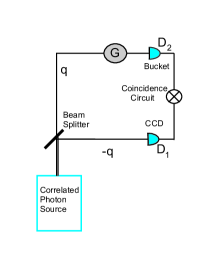
Figure 1: (Color online) Schematic depiction of correlated-photon imaging setup. The photons in the two arms have anticorrelated transverse momenta $\pm{\mathbf{q}}$.

We begin by briefly reviewing ghost imaging in section 2, followed by a review of aberration-cancelled interferometry in section 3. We then show how a small change converts the aberration-cancelled interferometer into a new type of ghost imaging system. We analyze this imaging system first with an entangled light source in section 4, then with a classical source in section 5. Finally, in section 6 we discuss an important technical point about the need for lenses in front of the detectors, followed by conclusions in section 7.

II CORRELATED-PHOTON IMAGING

Correlated-photon imaging or ”ghost” imaging pittman (1) is done with an apparatus like the one depicted schematically in figure 1. In the original version, the correlated photon source is a $\chi^{(2)}$ nonlinear crystal pumped by a laser, leading to SPDC. Entangled photon pairs with anticorrelated momentum components ${\mathbf{q}}$ and $-{\mathbf{q}}$ transverse to the propagation direction travel along the two arms of the apparatus. The object to be viewed is placed in arm 2 (the upper branch), followed by a bucket detector, $D_{2}$. $D_{2}$ can not record any information on the position or momentum of the photon that reached the object; it can only tell us whether or not the photon reached the detector unimpeded by an object. The other arm has no object, and all the photons reach a CCD camera or array of pointlike detectors without hindrance. A lens may be inserted in this branch for image formation. A coincidence circuit is used to record a count every time a photon detection occurs simultaneously (within a short time window) at each detector. By plotting the coincidence rate as a function of position ${\mathbf{x}_{1}}$ in detector 1, we build up an image of the object. This is true even though photons that actually encountered the object in branch 2 left no record of the object’s position, and the photons in branch 1 that do carry position information never encounter the object.

The crucial ingredient is the spatial correlation of the photon pair. It was found bennink1 (2, 3) that entanglement was unnecessary: a classical source with anticorrelated transverse momenta could mimic the effect. The correlated light source in this case consists of a beam steering modulator (a rotating mirror, for example) directing a classical light beam through a range of ${\mathbf{q}}$ vectors, illuminating different spots on the object. The beamsplitter turns the single beam of transverse momentum ${\mathbf{q}}$ into a pair of beams with momenta ${\mathbf{q}}$ and $-{\mathbf{q}}$. The results were similar to those with the entangled source, but with half the visibility. It was later shown that thermal and speckle sources may also lead to ghost imaging (gatti (4, 5, 6, 7, 8, 9)).

III SUMMARY OF ABERRATION CANCELLATION IN QUANTUM INTERFEROMETRY

Consider the setup shown in figure 2 bonato1 (13, 14, 15). Each branch contains a 4f imaging system with lenses of focal length $f$ and a thin object that provides spatial modulation $G_{j}({\mathbf{y}})$ of the beam, where $j=1,2$ labels the branch, and ${\mathbf{y}}$ is the position in the plane transverse to the axis. The goal is to cancel object-induced optical aberrations (position-dependent phase shifts produced by the $G_{j}$). The case of a single object in one branch only may be included by simply setting $G=1$ in the other branch. The plane of the samples (labelled $\Pi$ in fig. 2) is the Fourier plane of the 4f system. Time delay $\tau$ is inserted in one branch. In the detection stage, two large bucket detectors $D_{1}$ and $D_{2}$, connected in coincidence, record the arrival of photons, but not their positions. Apertures described by pupil functions $p_{1}({\mathbf{x}}_{1})$ and $p_{2}({\mathbf{x}}_{2})$ are followed by crossed polarizers at $45^{\circ}$ to each beam’s polarization, before arriving at the detectors.

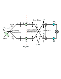
Figure 2: (Color online) Schematic of interferometer with even-order aberration-cancellation. Large bucket detectors $D_{1}$ and $D_{2}$ are integrated over and connected by a coincidence circuit.

A continuous wave laser pumps a $\chi^{(2)}$ nonlinear crystal, leading to collinear type II parametric downconversion. The frequencies of the two photons are $\Omega_{0}\pm\nu$, with transverse momenta $\pm{\mathbf{q}}$. For simplicity, assume the frequency bandwidth is narrow compared to $\Omega_{0}$. The two photons have total wavenumbers ${{\Omega_{0}\pm\nu}\over c}\approx{{\Omega_{0}}\over c}$. The downconversion spectrum is

$$\Phi({\mathbf{q}},\nu)=sinc\left[{{L\Delta({\mathbf{q}},\nu)}\over 2}\right]e^{i{{L\Delta({\mathbf{q}},\nu)}\over 2}},$$ (1)

where $L$ is the thickness of the crystal, and

$$\Delta({\mathbf{q}},\nu)=-\nu D+M\hat{\mathbf{e}_{2}}\cdot{\mathbf{q}}+{{2|{\mathbf{q}}|^{2}}\over{k_{pump}}}.$$ (2)

$D$ is the difference between the inverse group velocities of the ordinary and extraordinary waves in the crystal, and $M$ is the spatial walk-off in the direction $\hat{{\mathbf{e}_{2}}}$ perpendicular to the interferometer plane. The last term in $\Delta$ is due to diffraction in the crystal. Ignoring the vacuum term and terms of higher photon number, the wavefunction entering the apparatus is approximately given by

$$|\Psi\rangle = \int d^{2}q\;d\nu\;\Phi({\mathbf{q}},\nu)$$ (3)

$$\times\;\hat{a}_{s}^{\dagger}({\mathbf{q}},\Omega_{0}+\nu)\hat{a}_{i}^{\dagger}(-{\mathbf{q}},\Omega_{0}-\nu)|0\rangle,$$

where $\hat{a}_{s}$ and $\hat{a}_{i}$ are annihilation operators for the signal and idler photons. For collinear pairs, horizontally polarized photons are directed into the upper branch and vertically polarized photons into the lower branch by means of a polarizing beamsplitter. Alternatively, noncollinear pairs could be used with polarizers selecting horizontal (H) polarization in the upper branch and vertical (V) in the lower one. In either case, we will refer to the H photon in the upper branch (branch 2) as the signal and the V photon in branch 1 as the idler.

The coincidence rate is of the generic form rubin (16)

$$R(\tau)=R_{0}\left[1-\Lambda\left(1-{{2\tau}\over{DL}}\right)W(\tau)\right],$$ (4)

where $\Lambda(x)$ is the triangular function:

$$\Lambda(x)=\bigg{\{}\begin{array}[]{l}1-|x|,\qquad|x|\leq 1\\ 0,\qquad\qquad|x|>1\end{array}$$ (5)

For large apertures, $p_{1}({\mathbf{x}}_{1})=p_{2}({\mathbf{x}}_{2})\approx 1$; so, as shown in bonato2 (14), the background and $\tau$-modulation terms are

$$R_{0} = \int d^{2}q\left|G_{1}\left({{f{\mathbf{q}}}\over k}\right)G_{2}\left(-{{f{\mathbf{q}}}\over k}\right)\right|^{2}$$ (6)

$$W(\tau) = {1\over{R_{0}}}\int d^{2}qe^{-{{2iM\tau}\over D}{\mathbf{e}_{2}}\cdot{\mathbf{q}}}$$

$$\;\times\;G_{1}^{\ast}\left({{f{\mathbf{q}}}\over k}\right)G_{1}\left(-{{f{\mathbf{q}}}\over k}\right)$$

$$\times\;G_{2}^{\ast}\left(-{{f{\mathbf{q}}}\over k}\right)G_{2}\left({{f{\mathbf{q}}}\over k}\right),$$

where $k$ is the longitudinal wavenumber.

We may write $G_{j}({\mathbf{x}})=t_{j}({\mathbf{x}})e^{i\phi_{j}({\mathbf{x}})}$, with $t_{j}$ real. Aberration effects arise from spatially-dependent phase factors $\phi_{j}({\mathbf{x}})$, which lead to distortion of the outgoing wavefronts. The phase functions may be decomposed into a sum of pieces that are either even under reflection, $\phi_{j}^{(even)}(-{\mathbf{x}})=\phi_{j}^{(even)}({\mathbf{x}})$ or odd, $\phi_{j}^{(odd)}(-{\mathbf{x}})=-\phi_{j}^{(odd)}({\mathbf{x}})$. Astigmatism and spherical aberration, for example, are included in the even-order part, whereas coma is odd.

In equation (III), the factors $G_{1}^{\ast}\left({{f{\mathbf{q}}}\over k}\right)G_{1}\left(-{{f{\mathbf{q}}}\over k}\right)$ become

$$t_{1}^{\ast}\left({{f{\mathbf{q}}}\over k}\right)t_{1}\left(-{{f{\mathbf{q}}}\over k}\right)e^{-i\left[\phi_{1}\left({{f{\mathbf{q}}}\over k}\right)-\phi_{1}\left(-{{f{\mathbf{q}}}\over k}\right)\right]}.$$ (8)

the form of the difference in the exponent shows that even-order aberrations arising from object 1 cancel from the modulation term. The even-order aberrations from object 2 cancel in a similar manner. This is the even-order cancellation effect demonstrated in bonato1 (13) and bonato2 (14). As pointed out in simon1 (15), even- and odd-orders cancel simultaneously only in the special case $G_{1}=G_{2}$. These cancellations are exact only for aberrations induced by thin objects in the particular plane $\Pi$.

In the term $R_{0}$, both even-order and odd-order aberrations cancel even for $G_{1}\neq G_{2}$. For time correlation experiments, this is an unimportant background term; however this term is the foundation of the imaging apparatus described below, since the beamsplitter will be absent, meaning that there will be no modulation term $W(\tau)$. The physical mechanism of the various possible cancellations are discussed in more detail in simon1 (15).

IV ABERRATION-CANCELLED GHOST IMAGING WITH ENTANGLED SOURCE

Now we wish to look at the ghost imaging analog of the aberration-cancelling interferometer of the previous section. This leads us to the hybrid device of fig. 3. This new apparatus differs from that of fig. 2 in several respects. First, we have removed the time delay, polarization filters, and beam splitter; these were needed to produce the interference effects desired in bonato1 (13, 14, 15), but are not necessary for imaging purposes. Also, in order to obtain spatial resolution, one bucket detector ($D_{1}$) is replaced by a moveable pointlike detector or a CCD camera. The removal of the beam splitter and the introduction of spatial resolution are the key changes. After allowing for an arbitrary source of correlated (quantum or classical) light, we arrive at an apparatus in fig. 3 that looks very much like the ghost imaging setup of fig. 1, but with a 4f imaging system in each branch. In this section, we assume that the light source is parametric downconversion.

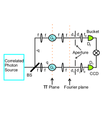
Figure 3: (Color online) Schematic of correlated-photon imaging setup with aberration-cancellation. All orders of aberration cancel.

The coincidence rate at location ${\mathbf{x}_{1}}$ of $D_{1}$ is

$$R({\mathbf{x}_{1}})=\int d^{2}x_{2}dt_{1}dt_{2}|A({\mathbf{x}_{1}},{\mathbf{x}_{2}},t_{1},t_{2})|^{2},$$ (9)

where the transition amplitude is

$$A({\mathbf{x}}_{1},{\mathbf{x}}_{2},t_{1},t_{2})=\langle 0|E_{1}^{(+)}({\mathbf{x}}_{1},t_{1})E_{2}^{(+)}({\mathbf{x}}_{2},t_{2})|\Psi\rangle.$$ (10)

Taking the two detection apertures described by $p_{1}$ and $p_{2}$ to be large, we compute the coincidence rate to be

$$R({\mathbf{x}_{1}}) = \left\{\left[B({\mathbf{x}_{1}})+B(-{\mathbf{x}_{1}})\right]+\left[C({\mathbf{x}_{1}})+C^{\ast}({\mathbf{x}_{1}})\right]\right\}$$ (11)

$$\quad\times\;\left|G_{1}\left({f\over{f_{D}}}{\mathbf{x}_{1}}\right)G_{2}\left(-{f\over{f_{D}}}{\mathbf{x}_{1}}\right)\right|^{2},$$

where

$$B({\mathbf{x}_{1}}) = \int d\nu\left|\Phi\left({{k{\mathbf{x}_{1}}}\over{f_{D}}},\nu\right)\right|^{2},$$ (12)

$$C({\mathbf{x}_{1}}) = \int d\nu\;\Phi\left({{k{\mathbf{x}_{1}}}\over{f_{D}}},\nu\right)\Phi^{\ast}\left(-{{k{\mathbf{x}_{1}}}\over{f_{D}}},-\nu\right).$$ (13)

Using eq. (1), these integrals may be evaluated; they turn out to be $x_{1}$-independent constants. Sweeping all overall constants into a single constant ${\cal R}_{0}$, we find:

$$R({\mathbf{x}_{1}})={\cal R}_{0}\left|G_{1}\left({f\over{f_{D}}}{\mathbf{x}_{1}}\right)G_{2}\left(-{f\over{f_{D}}}{\mathbf{x}_{1}}\right)\right|^{2}.$$ (14)

Only the modulus of each $G_{j}$ enters into $R({\mathbf{x}})$, so we see that the aberrations introduced by the object phases cancel to all orders. This will be exact only in the Fourier plane, but as was true for the interferometer case, we would expect it to continue to remain approximately true as we move out of the plane up to a maximum distance on the order of ${{fr_{s}}\over a}$, where $f$ and $a$ are the focal length and radius of the lens and $r_{s}$ is the maximum radius of the object being viewed. (See ref.(simon1 (15)) for a derivation of this estimate.)

If $G_{2}=1$, then we have an ordinary (non-ghost) image of $\left|G_{1}\right|$. On the other hand, if $G_{1}=1$ then we have an inverted ghost image of $\left|G_{2}\right|$. In either case, the image is magnified by a factor of $m={{f_{D}}\over f}$. Note that, in contrast to the interferometry case, even and odd order phases both cancel, even in the general case $G_{1}\neq G_{2}$. The cancellation of the phases only occurs in the Fourier plane; aberrative distortions begin growing when the objects are moved out of this plane.

V APPLICATIONS TO IMAGE ANALYSIS

Note that if both $G_{1}$ and $G_{2}$ are nontrivial objects, what we actually see is their pointwise product. This is a distinctive feature of this apparatus. It can be verified by straightforward calculation that the simple product structure of eq. (14) does not occur in other obvious variations of two-object ghost imaging systems; for example, it does not occur if the 4f imaging system in either branch (or both) is replaced by a single lens imaging system, or in a system without lenses. We may make use of this product structure in a number of ways. For example, if the object of interest is $G_{2}$ but the second branch introduces some known distortion to its image (e.g. there may be aberration in the optical system or variations in the refractive index of the propagation medium), then this can be cancelled by using an object $G_{1}$ that introduces an opposite distortion (via a deformable mirror, for example). The two distortions then cancel, leaving no net effect on the image. Alternatively, if $G_{2}$ has a dim, low-transmissivity area that we wish to view, but it is being obscured by a bright, high-transmissivity area nearby, we may use a mask for $G_{1}$ which allows a view only of the twins of photons coming from the dim region of interest, blocking photons that are partnered with light from other areas.

At first glance, the product structure might seem to open up a further interesting possibility. Suppose $G_{1}$ is the object we wish to view. If there is no object in branch 2 ($G_{2}$ is simply a constant), then the resolution with which we may view $G_{1}$ is the same as if the second branch was not there. It would be limited by the sizes of the Airy disks produced by the lenses. However, if $G_{2}$ is taken to be a small pinhole, the area we would be able to see of $G_{1}$ at any given time would be limited by the size of the pinhole. Thus, it would seem that by taking the pinhole small enough, we would be able to limit our view of $G_{1}$ to an area smaller than the standard Abbé limit, thus achieving subresolution imaging. Unfortunately, when the finite sizes of the lenses are properly taken into account (eq. (14) was derived in the limit of large lenses), the combined action of diffraction in the two branches conspires to give the single-branch resolution as its best-case limit, occurring when the pinhole radius is negligible. As the pinhole radius at $G_{2}$ grows to finite size, the resolution becomes worse than in the single-branch case.

One additional observation on applications of the product structure arises if we replace the position-resolving detector in branch 1 by a bucket detector, thus introducing an integration over ${\mathbf{x}_{1}}$. We have now lost all imaging ability, but note what happens if we displace one of the objects (object 1, say) by some distance in the transverse plane. If the 2-dimensional displacement vector is ${\mathbf{r}}$, then equation (14) is replaced by

$$R({\mathbf{r}})={\cal R}_{0}\int\left|G_{1}\left({f\over{f_{D}}}({\mathbf{x}_{1}}+{\mathbf{r}})\right)G_{2}\left(-{f\over{f_{D}}}{\mathbf{x}_{1}}\right)\right|^{2}dx_{1}.$$ (15)

Thus, despite the fact that neither detector has spatial resolution, the system optically computes the spatial intensity correlator $g({\mathbf{r}})=\langle I_{1}\left(m^{-1}({\mathbf{x}}+{\mathbf{r}})\right)I_{2}\left(-m^{-1}{\mathbf{x}})\right)\rangle$, where $m$ is the magnification. (The correlation here is actually between the object $G_{1}({\mathbf{x}})$ and the inverted object $G_{2}(-{\mathbf{x}})$, but an additional lens can be added to remove remove the inversion and cancel the minus sign in $G_{2}$.) The full correlation function can be found by moving one object repeatedly to scan over the full range of relevant ${\mathbf{r}}$ vectors. Taking one of the two objects to be unknown and the other to be some known template, this could provide a means of identifying the unknown object by quantifying its degree of similarity to the template. This could be useful, for example, in comparing silicon chips on an assembly line to a standard chip, and identifying those chips with flaws. Note in particular, that the unknown object may be in a remote, inaccessible location; for example, the object might be a cell inside the body being viewed through an endoscope and compared to a cell in the lab. As in the case of the temporal correlator studied with the interferometer of refs. bonato1 (13, 14, 15), the effect of object-induced aberrations (differences between phase shifts induced by the two samples) cancels out of the spatial correlator.

VI IMAGING WITH A CLASSICAL SOURCE

We now replace the downconversion source of the previous section by a classical source of anticorrelated photons, as in bennink1 (2). Light entering a beam splitter with transverse momentum ${\mathbf{q}}$ leads to outgoing beams with anticorrelated momenta ${\mathbf{q}}$ and $-{\mathbf{q}}$. If the beam steering modulator produces momentum spectrum $f({\mathbf{q}})$, the input state for pairs of photons having the same ${\mathbf{q}}$ before the beamsplitter will be $\sim\int d^{2}qF({\mathbf{q}})\hat{a}_{p}^{\dagger}({\mathbf{q}})\hat{a}_{p}^{\dagger}({\mathbf{q}})|0\rangle$, where $\hat{a}_{p}^{\dagger}$ is the creation operator for pump photons and $F({\mathbf{q}})\equiv f^{2}({\mathbf{q}})$. We assume for simplicity that $F({\mathbf{q}})$ is an even function, $F({\mathbf{q}})=F(-{\mathbf{q}})$. Denoting creation operators in the two outgoing branches by $\hat{a}_{1}^{\dagger}$ and $\hat{a}_{2}^{\dagger}$, the incoming photon pair will produce a state after the beamsplitter given by:

$$|\Psi\rangle = {1\over 2}\int d^{2}qF({\mathbf{q}})\left[\hat{a}_{1}^{\dagger}({\mathbf{q}})+\hat{a}_{2}^{\dagger}(-{\mathbf{q}})\right]$$

$$\qquad\qquad\qquad\qquad\times\left[\hat{a}_{1}^{\dagger}({\mathbf{q}})+\hat{a}_{2}^{\dagger}(-{\mathbf{q}})\right]|0\rangle$$

$$= \int d^{2}qF({\mathbf{q}})\left[\hat{a}_{1}^{\dagger}({\mathbf{q}})\hat{a}_{2}^{\dagger}(-{\mathbf{q}})+\;\dots\;\right]|0\rangle,$$ (17)

where the terms dropped in the last line are those which do not contribute to coincidence detection. The detection amplitude of eq. (10) is then proportional to

$$\int d^{2}qF({\mathbf{q}})e^{i{\mathbf{q}}\cdot({\mathbf{x}_{1}}-{\mathbf{x}_{2}})}H_{1}({\mathbf{q}},{\mathbf{x}_{1}})H_{2}(-{\mathbf{q}},{\mathbf{x}_{2}}),$$ (18)

where $H_{j}$ is the transfer function for branch $j$. Integrating over $D_{2}$, we then have the coincidence rate:

$$R({\mathbf{x}_{1}})=\left|F\left({k\over{f_{D}}}{\mathbf{x}_{1}}\right)G_{1}\left({f\over{f_{D}}}{\mathbf{x}_{1}}\right)G_{2}\left(-{f\over{f_{D}}}{\mathbf{x}_{1}}\right)\right|^{2}.$$ (19)

This is similar to the result for the entangled-source apparatus, except modulated by the factor $F\left({k\over{f_{D}}}{\mathbf{x}_{1}}\right)$ which is determined by the details of the beam steering modulator. Similarly, for thermal or speckle sources, this factor will arise from the transverse momentum spectrum of the source.

VII ROLE OF THE DETECTION LENS

Consider now the lenses immediately before the detectors in fig. 3. With no such detection lens present, the transfer function for branch $j$ would be

$$H_{j}({\mathbf{q}_{j}},{\mathbf{x}_{j}})=G_{j}\left({{f{\mathbf{q}_{j}}}\over k}\right)e^{i{\mathbf{q}}\cdot{\mathbf{\mathbf{x}_{j}}}},$$ (20)

from which we see that the information from each ${\mathbf{q}}$ value is spread over all ${\mathbf{x}}$ values. But with the lens, eq. (20) becomes

$$H_{j}({\mathbf{q}_{j}},{\mathbf{x}_{j}}) = e^{-{{ik{\mathbf{x}_{j}}^{2}}\over{2f_{D}}}\left({{d_{2}}\over{f_{D}}}-1\right)}e^{-{{id_{1}{\mathbf{q}_{j}}^{2}}\over{2k}}}$$ (21)

$$\times\;G_{j}\left({{f{\mathbf{q}_{j}}}\over k}\right)\delta\left({{k{\mathbf{x}_{j}}}\over{f_{D}}}-{\mathbf{\mathbf{q}_{j}}}\right),$$

so that each ${\mathbf{q}}$ value is localized at a single point in the detector plane via the delta function. Since each ${\mathbf{q}}$ value is also matched to an object point, the localization in the second case defines a mapping between points in the object plane and points in the detection plane, allowing reconstruction of an image by the pointlike detector $D_{1}$. This can be verified by computing the coincidence rate with or without the final lenses, i.e. using either eq. (20) or eq. (21). Doing so, we find that without the branch 1 lens the coincidence rate becomes independent of ${\mathbf{x}_{1}}$, making imaging impossible. In contrast, removing the branch 2 lens has no effect. This makes intuitive sense: we integrate over ${\mathbf{x}_{2}}$, so it does not matter if the momentum information in this branch is localized or spread over the entire detector. Thus we arrive at an important technical point: the lens before the bucket detector may be removed without harm, but the branch 1 lens is essential for imaging.

The need for a lens before $D_{1}$ may be viewed as follows. The 4f system in either branch transfers modulation $G_{j}$ from the transverse coordinate space (${\mathbf{x}}$) to the Fourier space (${\mathbf{q}}$), which is where the aberration cancellation actually takes place (see simon1 (15)). The lens in front of $D_{1}$ is then needed to transfer the modulation back to coordinate space for imaging.

VIII CONCLUSIONS

In conclusion, we have proposed a new type of two-object ghost imaging apparatus that cancels phase effects from thin objects in the vicinity of a particular plane and which allows comparisons between pairs of objects. The method involves a relatively simple apparatus and can be done with either entangled photon pairs or with a classically-correlated light source. This apparatus may have potential for new applications in biomedical research, industry, and other fields.

References

- (1) T.B. Pittman, Y.H. Shih, D.V. Strekalov, A.V. Sergienko, ”Optical imaging by means of two-photon quantum entanglement”, Phys. Rev. A 52, R3429-R3432 (1995).
- (2) R.S. Bennink, S.J. Bentley, R.W. Boyd, ” Two-Photon Coincidence Imaging with a Classical Source”, Phys. Rev. Lett. 89, 113601 (2002).
- (3) R.S. Bennink, S.J.Bentley, R.W. Boyd, J.C. Howell, ”Quantum and Classical Coincidence Imaging”, Phys. Rev. Lett. 92, 033601 (2004).
- (4) A. Gatti, E. Brambilla, M. Bache, L.A. Lugiato, ”Correlated imaging, quantum and classical”, Phys. Rev. A 70, 013802 (2004).
- (5) Y.J. Cai, S.Y. Zhu, ”Ghost imaging with incoherent and partially coherent light radiation”, Phys. Rev. E 71, 056607 (2005).
- (6) A. Valencia, G. Scarcelli, M. D’Angelo, Y.H. Shih, ”Two-Photon Imaging with Thermal Light”, Phys. Rev. Lett. 94, 063601 (2005).
- (7) G. Scarcelli, V. Berardi, Y.H. Shih, ”Can Two-Photon Correlation of Chaotic Light Be Considered as Correlation of Intensity Fluctuations?”, Phys. Rev. Lett. 96, 063602 (2006).
- (8) F. Ferri, D. Magatti, A. Gatti, M. Bache, E. Brambilla, L.A. Lugiato, ”High-Resolution Ghost Image and Ghost Diffraction Experiments with Thermal Light”, Phys. Rev. Lett. 94, 183602 (2005).
- (9) D. Zhang, ”Correlated two-photon imaging with true thermal light”, Opt. Lett. 30, 2354-2356 (2005).
- (10) J.D. Franson, ”Nonlocal cancellation of dispersion”, Phys. Rev. A 45, 3126-3132 (1992).
- (11) A.M. Steinberg, P.G. Kwiat, R.Y. Chiao, ”Dispersion cancellation in a measurement of the single-photon propagation velocity in glass”, Phys. Rev. Lett. 68, 2421-2424 (1992).
- (12) O. Minaeva, C. Bonato, B.E.A. Saleh, D.S. Simon, A.V. Sergienko, ”Odd- and Even-Order Dispersion Cancellation in Quantum Interferometry”, Phys. Rev. Lett. 102, 100504 (2009).
- (13) C. Bonato, A.V. Sergienko, B.E.A. Saleh, S. Bonora, P. Villoresi, ”Even-Order Aberration Cancellation in Quantum Interferometry”, Phys. Rev. Lett. 101, 233603 (2008).
- (14) C. Bonato, D.S. Simon, P. Villoresi, A.V. Sergienko, ”Multiparameter entangled-state engineering using adaptive optics”, Phys. Rev. A 79, 062304 (2009).
- (15) D.S. Simon, A.V. Sergienko, ”Spatial-dispersion cancellation in quantum interferometry”, Phys. Rev. A 80, 053813 (2009).
- (16) M.H. Rubin, D.N. Klyshko, Y.H. Shih, A.V. Sergienko, ”Theory of two-photon entanglement in type-II optical parametric down-conversion”, Phys. Rev. A 50, 5122-5133 (1994).