Perturbation of Gravitational Lensing

Abstract

A gravitational lens system can be perturbed by “rogue systems” in angular proximities but at different distances. A point mass perturbed by another point mass can be considered as a large separation approximation of the double scattering two point mass (DSTP) lens. The resulting effective lens depends on whether the perturber is closer to or farther from the observer than the main lens system. The caustic is smaller than that of the large separation binary lens when the perturber is the first scatterer; the caustic is similar in size with the large separation binary lens when the perturber is the last scatterer. Modelling of a gravitational lensing by a galaxy requires extra terms other than constanst shear for the perturbers at different redshifts. Double scattering two distributed mass (DSTD) lens is considered. The perturbing galaxy behaves as a monopole – or a point mass – because the dipole moment of the elliptic mass distribution is zero.

1 Introduction

The Galactic bulge is being surveyed for gravitational microlensing in search of microlensing planets. The lensing systems are the standard single scattering $n$-point mass lenses, where the bound system may consist of a single star, a multiple star, or a planetary system with one or two host stars. The Galactic bulge microlensing probability is $\sim 10^{-6}$ and the probability for an unbound system to be aligned with the main lensing system can be ignored because it is $\sim 10^{-12}$. The number of stars being surveyed is less than $10^{9}$. The lensing probability is proportional to the Einstein ring radius square, and the Einstein ring radius of the lensing toward the Galactic Bulge is characteristically $\sim 1$ mas. Thus, if we consider the probability of a “rogue” system to be within $1$ as from the main lensing system, the probability is $\sim 1$. In fact, ground-based microlensing events are known to be “plagued” with blending of light, and some of them other than the main lens itself can also be gravitationally relevant for the photon path. The perturbers can be dark as well.

The probability for the “rogue” system to be at the same distance as the main lens system is small where the “same distance” should be understood in the context that the two lens systems are within the coherence scale in which the lensing can be considered a single scattering lensing. Within the coherence scale, the probability for the photon path to weave through the two lenses can be ignored (Rhie and Bennett, 2010) (RB10 from here on). Thus it is most reasonable to assume in general that the two gravitationally unbound microlens systems are at different distances, and they would be best considered as a double scattering lensing system. Here it is assumed that the two lens elements are widely separated in the sky based on the argument in the previous paragraph and calculate the effects of the “rogue” system on the main lens. The double scattering lensing is a time-sequential process, and it matters whether the “rogue” system is farther away than the main lens from the observer or closer. The two cases are schematically shown in figure 1. By wide separation it is implied that the separation $\ell$ is much larger than the Einstein ring radius of the main lens.

We assume that the “rogue” perturbing system is a single point mass. The main lens of interest will be a single star, a multiple star, a planet system with one or two host stars, or a wide binary stars one of which hosts planets. Here we consider the most common and simplest case of a signle star and study the wide separation approximation of the double scattering two point mass (DSTP) lens. Then the most important effect of the perturbation is to break the degeneracy of the point caustic of the single lens to an extended caustic curve, and the size of the caustic will be the indicator of the influence of the perturber. It will be shown that the caustic size depends on the distances of the lenses and whether the perturber is in the front or in the back. When the perturber is the first scatterer, the caustic is smaller than that of the binary lens, and it is similar in size when the main lens is perturbed by a “rogue” system in front. A binary lens forms when the two lenses have the same distance – or within the coherence length. The binary lens at large separation is made of a point mass and a constant shear (and plus the source shift), and it is briefly discussed in the appendix.

A multiple-point mass lens perturbing a single point mass main lens is approximated by the same form of the approximate DSTP lens equation (with effective coefficients) and can be concluded to behave in the similar manner to the single point mass perturber.

In lensing by a galaxy, modelling is done customarily by assuming an elliptic mass (sometimes replaced by an elliptic potential) and a constant shear. The galaxy lensing is of order $1$ arcsecond, and there are often other galaxies in the angular vicinity of the main lens system. The perturbers can be group memebers of the main lens or galaxies at different distances. If there is a perturbing galaxy at the same distance, its monopole will add an external shear as is the case with the binary lens. However, if the perturbing masses are at different distances, the perturbation should include deflection terms other than the constant external shear. We consider the wide separation approximation of the double scattering two distributed mass (DSTD) lens. The other terms depend on the double scattering parameter and vanish when the perturbers are at the same distance as the main lens because the double scattering parameter vanishes. The perturbation by an elliptic mass galaxy is approximated by the perturbation by a point mass (monopole) because the dipole moment of the elliptic mass distribution is zero. The main lens galaxy, assumed to have an elliptic mass distribution, has a finite size caustic, and the effect of the perturber is to change its shape, size, and position. Even in the simpler case of the main galaxy as the monopole-quadrupole lens requires numerical calculations. We leave the perturbations of the finite size caustics for future work.

It should be necessary to point out that Keeton (2003) uses Taylor expansion and concludes that the effects of a perturbing mass on the galaxy lens is to add constant convergence and constant shear irrelevantly of whether the perturber is the first scatterer or the last. There may be a problem in the expansion cutoff. In the region of interest around the critical curve of the galaxy lens, the first term in the Taylor expansion is small because the Jacobian determinant is zero or small and is likely to be smaller than the second order term. The second order term is well known for the square root behavior of the lensing near the critical curve or caustic crossing. It is not clear whether the Taylor expansion can be used at all. We use power expansion around the critical curve of the main lens which is the region of interest.

The DSTD lens equation is an obvious extension of the DSTP lens equation in which the delta function integral for the 2-d gravitational field of a point mass is generalized to the density function integral for the 2-d gravitational field of the distributed mass.

The DSTP lens equation is known since 1986 (Blandford and Narayan) and have been studied (Kochanek and Apostolakis, 1986; Erdl and Schneider, 1993; Werner et al, 2008). Here the derivation of the DSTP lens equation studied in RB10 is briefed for clarity and convenience. Instead of using the formula for the time delay and Fermat principle, the well-known derivation of the single lens equation from an exact solution of the general relativity, the Schwarzschild metric, with the assumption of the linear gravity and small angle approximation is used. The Schwarzschild metric is asymptotically flat and the scattering planes can be joined easily in the asymptotic regions. The DSTP lens equation is obtained by joining two scattering planes with the freedom to rotate.

2 The DSTP Lens Equation

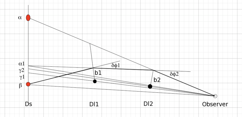
Figure 2: A diagram of a photon path scattered by lenses 1 and 2 at distances $D_{l1}$ and $D_{l2}$ in sequence. The scattering planes are noncoplanar in general, and the angles should be considered as two-vectors in three space.

The double scattering two point lens equation can be obtained from a diagram shown in figure 2 where the linear gravity and small angle approximation are assumed. Since the true photon path is three dimensional because of the rotation of the scattering planes with respect to each other, a three-dimensional diagram is needed. But it has been shown in RB10 that in the linear approximation in small angles, the radial component (in the direction of the line of sight) of the impact vector that is generated due to the relative rotation of the scattering planes can be ignored because it is of the second order. It is sufficient to express the triangular relations of the angles in vectors to account for the relative rotaion between the two scattering planes.

From figure 2 two sets of relations are obtained.

$$\vec{b}_{1}=D_{l1}(\vec{\alpha}-\vec{\gamma}_{1})+(D_{l1}-D_{l2})\vec{\delta}\varphi_{2}\ ;\qquad D_{s}(\vec{\alpha}_{1}-\vec{\beta})=-\vec{\delta}\varphi_{1}(D_{s}-D_{l1})$$ (1)

$$\vec{b}_{2}=D_{l2}(\vec{\alpha}-\vec{\gamma}_{2})\ ;\qquad D_{s}(\vec{\alpha}-\vec{\alpha}_{1})=-\vec{\delta}\varphi_{2}(D_{s}-D_{l2})$$ (2)

where the bending (scattering) angles are given by the point mass bending angles.

$$\vec{\delta}\varphi_{1}=\frac{4GM_{1}(-\hat{b}_{1})}{b_{1}}\ ;\qquad\vec{\delta}\varphi_{2}=\frac{4GM_{2}(-\hat{b}_{2})}{b_{2}}\$$ (3)

$M_{1}$ and $M_{2}$ are the masses of the first and second point mass scatterers at the distances $D_{l1}$ and $D_{l2}$, and $D_{s}$ is the distance to the source; $\vec{b}_{1}$ and $\vec{b}_{2}$ are the impact vectors, and $b_{1}\equiv|\vec{b}_{1}|$ and $b_{2}\equiv|\vec{b}_{2}|$. The lens equation is obtained from the second equations of eqs. (1) and (2),

$$D_{s}(\vec{\alpha}-\vec{\beta})=-\vec{\delta}\varphi_{1}(D_{s}-D_{l1})-\vec{\delta}\varphi_{2}(D_{s}-D_{l2})\,,$$ (4)

which is completed by using eq.(3) and the first equations of eqs. (1) and (2).

It is convenient (or our custom) to define a lens plane and use linear variables instead of the angular variables. Note that the intermediate image position angle $\vec{\alpha}_{1}$ was defined by projecting the intermediate photon ray back to the sky at the distance of the source. So define the lens plane, where the lens equation variables are defined, as the plane at the distance of the source and normal to a chosen radial direction. The lens equation is independent of the choice of the radial direction because of the linear approximation in small angle. Since the lens plane is placed at the distance of the source, the linear variables are $D_{s}$ times the angular variables.

Now employ the complex coordinates as usual and let $\omega$, $z$, and $x_{j}:j=1,2$ denote the (2-dimensional) positions (on the lens plane at the distance of the source) of a source, an image, and lenses $1$ and $2$. Then the lens equation in eq.(4) can be written in terms of the linear variables.

$$\omega=z-\frac{r_{E1}^{2}}{\bar{z}_{1}-{r_{E21}^{2}}z_{2}^{-1}}-\frac{r_{E2}^{2}}{\bar{z}_{2}}\,,$$ (5)

where $z_{j}\equiv z-x_{j}:\ j=1,2$. Let $r_{Ekj}$ be the (single lens) Einstein ring radius of the lensing by object $k$ of object $j$, and let object $0$ refer to the source. $r_{E1}\equiv r_{E10}$, $r_{E2}\equiv r_{E20}$, and $r_{E21}$ are as follows.

$$r_{E1}^{2}=4GM_{1}D_{1}\frac{D_{s}^{2}}{D_{l1}^{2}}=R_{E1}^{2}\frac{D_{s}^{2}}{D_{l1}^{2}};\qquad D_{1}\equiv\frac{D_{l1}(D_{s}-D_{l1})}{D_{s}}$$ (6)

$$r_{E2}^{2}=4GM_{2}D_{2}\frac{D_{s}^{2}}{D_{l2}^{2}}=R_{E2}^{2}\frac{D_{s}^{2}}{D_{l2}^{2}};\qquad D_{2}\equiv\frac{D_{l2}(D_{s}-D_{l2})}{D_{s}}$$ (7)

$$r_{E21}^{2}=4GM_{1}D_{3}\frac{D_{s}^{2}}{D_{l2}^{2}}=R_{E21}^{2}\frac{D_{s}^{2}}{D_{l2}^{2}};\qquad D_{3}\equiv\frac{D_{l2}(D_{l1}-D_{l2})}{D_{l1}}$$ (8)

$D_{j}:j=1,2,3$ are the reduced distances, and $R_{Ekj}$ is the “intrinsic” Einstein ring radius of the lensing of object $j$ by object $k$. The reason why we refer to $R_{Ekj}$ as the intrinsic Einstein ring radius is that the photon rays of the Einstein ring image of the lensing (of object $j$ by object $k$) actually pass through the ring around the lens ($k$) of radius $R_{Ekj}$ (accurate within the small angle approximation).

Redefine distances $D_{j1}\equiv D_{lj}$ and $D_{j2}\equiv D_{s}-D_{lj}$ and define effective masses

$$effM_{j}\equiv M_{j}\frac{D_{j2}}{D_{j1}}\ :\qquad j=1,2\ .$$ (9)

Define the Einstein ring radius $r_{E}$ of the total effecitve mass,

$$r_{E}^{2}\equiv r_{E1}^{2}+r_{E2}^{2}=4GD_{s}(effM_{1}+effM_{2})\,,$$ (10)

and the lens equation can be normalized so that the unit distance is $r_{E}$. By substituing $\omega$, $z$ and $x_{j}$ in eq.(5) by $r_{E}\omega$, $r_{E}z$ and $r_{E}x_{j}$ respectively, the normalized lens equation is obtained.

$$\omega=z-\displaystyle\frac{\epsilon_{1}}{\bar{z}_{1}-\displaystyle\frac{a}{z_{2}}}-\frac{\epsilon_{2}}{\bar{z}_{2}}\,,$$ (11)

where the effective fractional masses are

$$\epsilon_{1} \equiv\displaystyle\frac{r_{E1}^{2}}{r_{E}^{2}}=\displaystyle\frac{effM_{1}}{effM_{1}+effM_{2}}=\displaystyle\frac{M_{1}}{M_{1}+M_{2}/d}=\displaystyle\frac{\epsilon}{1+\epsilon}$$ (12)

$$\epsilon_{2} \equiv\displaystyle\frac{r_{E2}^{2}}{r_{E}^{2}}=\displaystyle\frac{effM_{2}}{effM_{1}+effM_{2}}=\displaystyle\frac{M_{2}}{M_{1}d+M_{2}}=\displaystyle\frac{1}{1+\epsilon}$$ (13)

and the double scattering parameter is

$$a\equiv\displaystyle\frac{r_{E21}^{2}}{r_{E}^{2}}=\displaystyle\frac{M_{2}(1-d)}{M_{1}d+M_{2}}=\frac{1-d}{1+\epsilon}$$ (14)

The distance parameter $d$ is

$$d\equiv\frac{D_{12}D_{21}}{D_{11}D_{22}}\ \ \leq\ 1$$ (15)

where the equality in the second relation holds when the two lenses are at the distance. The effective mass ratio $\epsilon$ is

$$\epsilon\equiv\frac{\epsilon_{1}}{\epsilon_{2}}=\frac{r_{E1}^{2}}{r_{E2}^{2}}=\frac{effM_{1}}{effM_{2}}=d\frac{M_{1}}{M_{2}}$$ (16)

The effective mass ratio is smaller than the mass ratio. The weight is shifted to the last scatterer in double scattering lensing. Note that we have chosen the last scatterer for the reference mass.

It should be worth pointing out that the double scattering parameter $a$ is essentially the (square of the) Einstein radius that is easily measurable in an (almost) axisymmetric system as in SDSSJ0946+1006 (Gavazzi et al, 2008). In an axisymmetric DSTP lens three ring images are formed, even though the innermost ring is “unstable” to break into a half-circle, and $\sqrt{a}$ measures the middle ring radius in units of the Einstein ring radius of the total effective mass $r_{E}$. The DSTP lens system can be considered to have two characteristic parameters $r_{E}$ and $\sqrt{a}$.

Here the focus is in the main lens and the interest is on what happens to the Einsteing ring of the main lens under the perturbation of a perturbing mass. So it is useful to renormalize the lens equation by the Einstein ring radius of the main lens. There are two cases: 1) object 1 is the perturbing mass; 2) object 2 is the perturbing mass.

Case 1): Renormalize the lens equation (11) so that the unit distance is $r_{E2}$.

$$\omega=z-\frac{\epsilon}{\bar{z}_{1}-\tilde{a}_{2}z_{2}^{-1}}-\frac{1}{\bar{z}_{2}}$$ (17)

where

$$\tilde{a}_{2}\equiv\frac{r_{E21}^{2}}{r_{E2}^{2}}=1-d$$ (18)

Case 2): Renormalize the lens equation so that the unit length is $r_{E1}$.

$$\omega=z-\frac{1}{\bar{z}_{1}-\tilde{a}_{1}z_{2}^{-1}}-\frac{\epsilon^{-1}}{\bar{z}_{2}}$$ (19)

where

$$\tilde{a}_{1}\equiv\frac{r_{E21}^{2}}{r_{E1}^{2}}=\frac{1-d}{\epsilon}$$ (20)

3 Large Separation DSTP Lenses: $\ell>>1$

3.1 When the Perturber is the First Scatterer

3.1.1 The Lens Equation

Let the separation be denoted by $\ell\equiv|x_{1}-x_{2}|$. The coordinate system can be chosen such that lens 2 is at the origin, $x_{2}=0$, and lens 1 is on the positive side of the real axis, $x_{1}=\ell$. Since it is assumed that $\ell>>1$, the lens equation (17) can be expanded in power series in $\ell^{-1}$, assuming that $\epsilon$ is not bigger than ${\cal O}(1)$, to obtain the following.

$$\omega-\frac{\epsilon}{\ell}=z-\frac{1}{\bar{z}}+\frac{\epsilon}{\ell^{2}}\bar{z}-\frac{\epsilon}{\ell^{2}}\frac{\tilde{a}_{2}}{z}$$ (21)

The lens is made of a point mass ($\propto 1/\bar{z}$), a constant shear ($\propto\bar{z}$), and a mass-antimass distribution($\propto 1/z$); the source is shifted by $\epsilon/\ell$ as is the case with the wide separation binary lens. (See appendix.) Consider the RHS minus the LHS as a vector field. It is a vector field with zeros and poles on the two sphere, and the index of the vector field at $z\sim\infty$ results in $n_{+}-n_{-}=0$ where $n_{+}$ and $n_{-}$ are the number of positive and negative images respectively. (See RB10.) Thus, the number of images is even and the number of negative images is the same as the number of positive images. There are two images for $\omega=\infty$, namely $z=0$ and $\infty$, hence there are two or four images where the latter occurs inside the finite size caustic. The finite size caustic occurs because the degeneracy of the point caustic of the single lens is broken by the perturbation of the mass $M_{1}$. The size of the caustic curve is calculated below using second order approximation in $\ell^{-1}$.

3.1.2 The Critical Curve and Caustic Curve

The Jacobian of the lens equation is given as

$$Jacobian=\pmatrix{f\ g\cr\bar{g}\ \bar{f}}\ :$$ (22)

$$f\equiv\partial\omega=1+\frac{\epsilon}{\ell^{2}}\frac{\tilde{a}_{2}}{z^{2}};\qquad g\equiv\bar{\partial}\omega=\frac{\epsilon}{\ell^{2}}+\frac{1}{\bar{z}^{2}}.$$ (23)

where $\partial\equiv\partial/\partial z$ and $\bar{\partial}\equiv\partial/\bar{\partial}z$. The Jacobian determinant is

$$J=|f|^{2}-|g|^{2}$$ (24)

and the eigenvalues of the Jacobian are

$$\lambda_{\pm}=f_{R}\pm\left(|g|^{2}-f_{I}^{2}\right)^{1/2}$$ (25)

where $f_{R}$ and $f_{I}$ are the real and imaginary parts of $f$. On the critical curve, where $J=0$, one or both of the eigenvalues are zero because $J$ is the product of the eigenvalues.

$$\lambda_{\pm}=f_{R}\pm f_{R}$$ (26)

Thus $\lambda_{-}$ vanishes on the critical curve, and $\lambda_{+}$ also vanishes if $f_{R}=0$. Note that $f=f_{R}=1$ in the case of the binary lens, and $\lambda_{+}$ never vanishes. Here $f_{R}>0$ because $\ell>>1$.

The lens system is simple enough so that the critical curve can be explicitly written out as a simple function. If we set $z=re^{i\theta}$, the critical condition is given by the following in the linear approximation in $\epsilon/\ell^{2}$.

$$r=1+\frac{\epsilon d}{2\ell^{2}}\cos 2\theta$$ (27)

Compared to the circular critical curve $r=1$ of the main (single) lens, the critical curve is slightly squeezed in a quadrupolar manner. Note that every point of the entire ring $r=1$ of the single lens is a precusp (i.e., mapped to a cusp). The curve in eq.(27) is circular ($dr/d\theta=0$) at four points: $0$, $\pi/2$, $\pi$, and $3\pi/2$, and they are expected to be the precusps. It is the indeed the case as will be shown shortly. The size of the caustic can be estimated by calculating the cusp positions using the lens equation. The precusps along the real axis, $\theta=0$ and $\pi$, are mapped to cusp points on the real axis, and the length of the caustic along the real axis is obtained as the difference between the cusp positions.

$$\Delta\omega_{real}=\omega(x)-\omega(-x)=\frac{4\epsilon d}{\ell^{2}};\qquad x=1+\frac{\epsilon d}{2\ell^{2}}$$ (28)

The length of the caustic in the direction parallel to the imaginary axis is given as the absolute value of the following.

$$\Delta\omega_{imag}=\omega(iy)-\omega(-iy)=-i\frac{4\epsilon d}{\ell^{2}};\qquad y=1-\frac{\epsilon d}{2\ell^{2}}$$ (29)

$$|\Delta\omega_{real}|=|\Delta\omega_{imag}|=\frac{4}{\ell^{2}}\frac{M_{1}}{M_{2}}d^{2}$$ (30)

Thus the quadroid caustic is equilateral and the orientation of the caustic is opposite to the critical curve. In comparison to the wide separation binary lens, for which $d=1$, the size of the caustic is smaller by factor $d^{2}$. See the Appendix for the wide separation binary. If the lens elements are evenly distributed in distance between the observer and the source, then $d=1/4$, and the caustic shrinks by $1/16$. It is substantial, and it demonstrates that perturbation of microlensing events by a “rogue” mass in an angular proximity should be estimated by using a proper double scattering lens equation. It has been the practice that all possible perturbers are universally thrown into constant shear corrections, or constant shear and constant convergence.

3.1.3 Cusps

On the critical curve, $f_{R}>0$, hence $\lambda_{-}=0$ is responsible for $J=0$. Thus, if $e_{+}$ and $e_{-}$ are the eigenvectors coresponding to $\lambda_{+}$ and $\lambda_{-}$ respectivley, then $e_{-}$ is the critical direction. If we consider drawing the caustic curve by mapping the critical curve by the lens equation, only the non-critical ($e_{+}$) component of the tangent vector of the critical curve is mapped to the tangent of the caustic curve because of the criticality condition. Thus the caustic curve is tangent to the eigendirection of $\lambda_{+}$ (Rhie, 1999, 2001). If the tangent to the critical curve is parallel to the critical direction, the tangent mapped to the caustic curve is zero and the progression of the caustic curve stops and forms a cusp. In the next moment, the non-critical component is picked up and the caustic curve turns around changing the direction by $\pi$. If $p$ is the parameter of the critical curve, the tangent to the curve is determined by

$$0=\frac{dJ}{dp}=\frac{dz_{+}}{dp}\partial_{+}J+\frac{dz_{-}}{dp}\partial_{-}J$$ (31)

where $dz_{\pm}$ are the increments in the $\pm$ eigendirections. The cusp forms when $dz_{+}/dp=0$, hence $0=\partial_{-}J$. The (unnormalized) eigenvectors are

$$e_{+}\propto\pmatrix{u_{+}\cr v_{+}};\qquad e_{-}\propto\pmatrix{u_{-}\cr v_{-}},$$ (32)

where we can choose $u_{\pm}$ and $v_{\pm}$ as

$$u_{+}=g\ ;\qquad v_{+}=-if_{I}+\left(|g|^{2}-f_{I}^{2}\right)^{1/2}$$ (33)

$$u_{-}=g\ ;\qquad v_{-}=-if_{I}-\left(|g|^{2}-f_{I}^{2}\right)^{1/2}$$ (34)

The Jacobian matrix can be diagnolized using $\Lambda$ constructed from the eigenvectors components,

$$\Lambda=\pmatrix{u_{+}\ u_{-}\cr v_{+}\ v_{-}}:\qquad\Lambda^{-1}(Jacobian)\Lambda=\pmatrix{\lambda_{+}\ 0\cr 0\ \lambda_{-}},$$ (35)

and the eigendirection differentials can be written as

$$\pmatrix{dz_{+}\cr dz_{-}}=constant\,\Lambda^{-1}\pmatrix{dz\cr d\bar{z}}$$ (36)

where $constant$ is a real constant. Thence $\partial_{-}z=constant\ u_{-}$ and and $\partial_{-}\bar{z}=constant\ v_{-}$, and the cusps are found from the cusp condition.

$$0=\partial_{-}J=\partial_{-}z\partial J+\partial_{-}\bar{z}\bar{\partial}J\qquad\Rightarrow\qquad 0=u_{-}\partial J+v_{-}\bar{\partial}J$$ (37)

Straightforward calculations show that, in the second order in $\ell^{-1}$, $\partial_{-}J=0$ for $\theta=0$, $\pi/2$, $\pi$, and $3\pi/2$ of the critical curve in eq.(27). Therefore they are precusps in the second order approximation.

3.1.4 Images

Set $z=re^{i\theta}$ and $\zeta=\omega-\epsilon/\ell$. The lens equation for the shifted source position is given by

$$\zeta=\xi e^{i\theta}+\eta e^{-i\theta}$$ (38)

where $\xi$ and $\eta$ are functions of $r$.

$$\xi=r-\frac{1}{r};\qquad\eta=\frac{\epsilon}{\ell^{2}}\left(r-\frac{\tilde{a}_{1}}{r}\right)$$ (39)

If we let $\zeta=\zeta_{1}+i\zeta_{2}$,

$$\zeta_{1}=(\xi+\eta)\cos\theta;\qquad\zeta_{2}=(\xi-\eta)\sin\theta,$$ (40)

and an equation for $r$ is obained.

$$\left(\frac{\zeta_{1}}{\xi+\eta}\right)^{2}+\left(\frac{\zeta_{2}}{\xi-\eta}\right)^{2}=1$$ (41)

There are two or four solutions to the equation (41), which indicates that there are two solutions outside the quadroid caustic and four solutions inside the caustic. When the source is inside the caustic, the images are all at $r\approx 1$. They are the four bright images that form around the critical curve $r\approx 1$, two outside the critical curve in the area of the “squeezed” and two inisde the critical curve in the area of the “bulged”. For example, $\zeta=0$ is inside the caustic, and the four images are on the real axis and the imaginary axis.

$$r_{1,2}^{2}=1+\frac{\epsilon}{\ell^{2}}(1-\tilde{a}_{2})\ ;\qquad\theta_{1}=\frac{\pi}{2},\quad\theta_{2}=\frac{3\pi}{2}$$ (42)

$$r_{3,4}^{2}=1-\frac{\epsilon}{\ell^{2}}(1-\tilde{a}_{2})\ ;\qquad\theta_{3}=0,\quad\theta_{4}=\pi$$ (43)

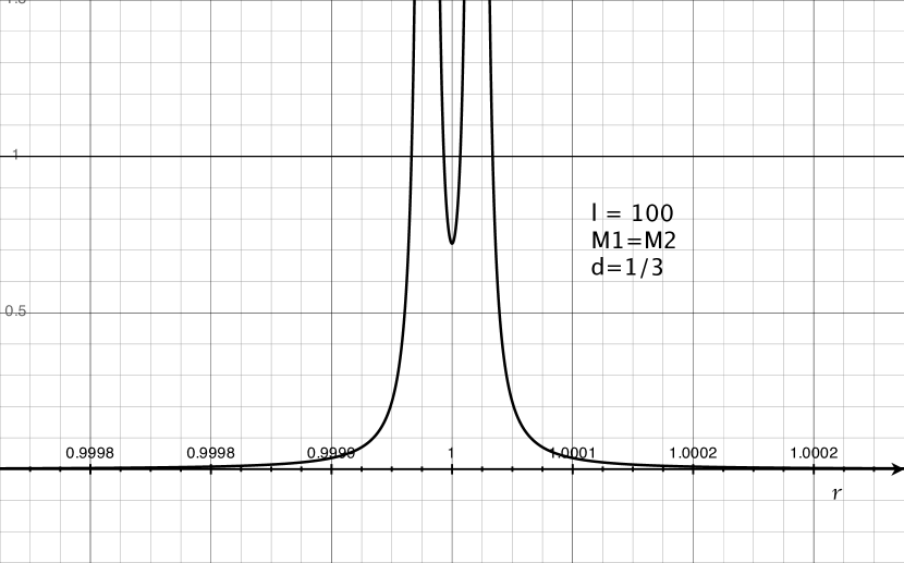
Figure 3: The radii of the four images of a source at $\zeta_{1}=\zeta_{2}=2\times 10^{-5}$. They are all near 1 – the Einstein ring radius of the main lens $M_{2}$. The lens parameters are $\ell=100$, $d=1/3$, and $M_{1}=M_{2}$.

The radius $r_{1,2}$ is bigger than $r_{3,4}$ because $\tilde{a}_{2}<1$ for a double scattering lens with $d<1$. Generally, the radii of the images are different. Figure 3 shows a case: $\ell=100$, $d=1/3$, and $M_{1}=M_{2}$; $\zeta_{1}=\zeta_{2}=2.\times 10^{-5}$. The angle $\theta$ for the radius $r$ of each image is determined from eq.(40). The four images of a finite size source filling the caustic form more or less a circular ring with finite thickness threaded by $r=1$.

3.2 When the Perturber is the Last Scatterer

3.2.1 The Lens Equation

Power-expand eq.(19) in $\ell^{-1}$ assuming $|z|\approx 1$ because we are interested in the region around the critical curve. Keep the terms up to the second order in $\ell^{-1}$ because the size of the caustic is of the second order. It will be shown that the linear order perturbation shifts the position of the caustic, by $d(\epsilon\ell)^{-1}$, but does not break the degeneracy of the point caustic.

$$\omega-\frac{1}{\epsilon\ell}=z-\frac{1}{\bar{z}}+\frac{\tilde{a}_{1}}{\ell\bar{z}^{2}}+\frac{\tilde{a}_{1}z}{\ell^{2}\bar{z}^{2}}-\frac{\tilde{a}_{1}^{2}}{\ell^{2}\bar{z}^{3}}+\frac{\bar{z}}{\epsilon\ell^{2}}$$ (44)

The lens is made of a point mass, a constant shear, and a whole variety of multipoles. From the index of the vector field with zeros and poles, it is obtained that $n_{+}-n_{-}=-2$ where $n_{\pm}$ is the number of positive/negative images. Thus the number of images is even. For $\omega=\infty$, there are four images, one at $z=\infty$ and three degenerate images at $z=0$. As $\omega$ moves toward the lenses, the three degenerate images individualizes. It is expected that the number of images is four outside the caustic and six inside so that $n_{+}-n_{-}=-2$. It is known that the original lens equation (eq.(17) or (19)) without approximations produces four or six images (Erdl and Schneider, 1993; Petters, 1997), and RB10 succeeded in deriving the sixth order analytic polynomial equation from the lens equaiton. However, the approximate lens equation (44) has a third order pole, and we will see that two images are dark images remaining near the pole. We refer to them as ignorable images.

3.2.2 The Critical Curve and Caustic

Jacobian matrix components are

$$f=\partial\omega=1+\frac{\tilde{a}_{1}}{\ell^{2}\bar{z}^{2}};\qquad g=\bar{\partial}\omega=\frac{1}{\bar{z}^{2}}-\frac{2\tilde{a}_{1}}{\ell\bar{z}^{3}}-\frac{2\tilde{a}_{1}z}{\ell^{2}\bar{z}^{3}}+\frac{3\tilde{a}_{1}^{2}}{\ell^{2}\bar{z}^{4}}+\frac{1}{\epsilon\ell^{2}}.$$ (45)

Set $z=re^{i\theta}$ and the Jacobian determinant $J=|f|^{2}-|g|^{2}$ can be computed up to the second order.

$$J=1-\frac{1}{r^{4}}+\frac{4\tilde{a}_{1}\cos\theta}{\ell r^{5}}+\frac{2\tilde{a}_{1}\cos\theta}{\ell^{2}}\left(\frac{1}{r^{2}}-\frac{2}{r^{4}}\right)-\frac{2\cos\theta}{\epsilon\ell^{2}r^{2}}-\frac{4\tilde{a}_{1}^{2}}{\ell^{2}r^{6}}-\frac{6\tilde{a}_{1}^{2}\cos 2\theta}{\ell^{2}r^{6}}$$ (46)

In the linear order,

$$J_{linear}=1-\frac{1}{r^{4}}\left(1-\frac{4\tilde{a}_{1}\cos\theta}{\ell r}\right),$$ (47)

and the critical curve, $J_{linear}=0$, is given by

$$\frac{4\tilde{a}_{1}\cos\theta}{\ell}=r-r^{5};\qquad r\neq 0.$$ (48)

Using graph of the RHS and the fact that $|\cos\theta|\leq 1$, it is found that the solution space is near $r=0$ and $r=1$. We are interested in the critical curve with $r\approx 1$. Let $r=1-\delta$ and obtain the critical curve in the linear order in $\delta$.

$$r=1-\frac{\tilde{a}_{1}\cos\theta}{\ell}.$$ (49)

It is a cardioid even though it is hard to distinguish from a circle because of the small coefficient of the $\cos\theta$ term. The whole critical curve is mapped by the approximate lens equation (44) to a point $\omega=d(\epsilon\ell)^{-1}$, hence the caustic is a point caustic in the linear order. It is shifted from that of the single lens. The position is different by factor $d$ from the center of the caustic of the large separation binary lens which is $(\epsilon\ell)^{-1}$.

We need the second order, and the second order depends on $\cos 2\theta$. The combination of $\cos\theta$ terms and $\cos 2\theta$ terms produces an “egg-shape” curve that resembles the familiar quaroid critical curve of the binary lens. Set $r=1-\delta$ and

$$\delta=\frac{A}{\ell}+\frac{B}{\ell^{2}}$$ (50)

and find $A$ and $B$ from the full Jacobian determinant in eq.(46).

$$A=\tilde{a}_{1}\cos\theta\ ;\qquad B=\frac{3\tilde{a}_{1}}{2}\cos 2\theta-\frac{1}{2\epsilon}\cos 2\theta+\frac{\tilde{a}_{1}^{2}}{4}(1-\cos 2\theta)$$ (51)

The critical curve $r(\theta)$ is a linear function of $\cos\theta$ and $\cos 2\theta$, hence it has the shape of an asymmetric peanut (squeezed in at $\theta=0$ and $\pi$) or a pear depending on whether the coefficient of $\cos 2\theta$ is negative or positive. (The coefficient of $\cos\theta$ is negative.)

For $\theta=0$ and $\pi$, $dr/d\theta=0$, and they are suspected to be precusps. They are, as can be shown by calculating $\partial_{-}J$ as was done for case 1). The other two precusps can be seen numerically to occur not exactly but practically at $\theta=\pi/2$ and $3\pi/2$. The cusps on the real axis will be used to estimate the size of the caustic.

$$\Delta\omega_{real}=\omega_{0}-\omega_{\pi}=\frac{4d}{\epsilon\ell^{2}}=\frac{4}{\ell^{2}}\frac{M_{2}}{M_{1}}$$ (52)

It is of order $1/\ell^{2}$ and is the same size as the large separation binary lens. But the shape of the critical curve is different from that of a binary lens as was mentioned above. Such a nice result should have a physical interpretation which escapes our mind currenlty. It should be worth pondering in an idle time.

The majority of the microlensing toward the Galactic bulge is bulge-bulge lensing and the microlensing event can be perturbed by a foregroud star. The highest magnification microlensing event observed to date is of the total magnification 2400, which means that the impact distance is $4.17\times 10^{-4}$ Einstein ring radius. If $M_{1}=M_{2}$ and $\ell=100$, then the “radius” of the caustic is $2\times 10^{-4}$. If the main lens has solar mass and is at $D_{l1}=3D_{s}/4$, the Einstein ring radius is $r_{E1}=2310sec$. If the source star is a sun-like star with the solar radius ($2.32$ sec), it is $10^{-3}$ in units of the Einstein ring radius. The caustic is completely inside the source star radius. Thus perturbers with $\ell\hbox{ \hbox to0.0pt{\raise 1.82986pt\hbox{$<$}\hss}\lower 2.79857pt\hbox{$\sim$} }1/100$ are expected to contribute to measurable effects. Of course, a more massive perturber (large $M_{2}$) perturbs more strongly, and when it is much larger than the main lens, the calculations done here are not proper because we would need higher order terms.

3.2.3 Cusps

In order to see that the critical points given by eq.(46) are precusps where $\theta=0$ and $\pi$, calculate $\partial_{-}J$ for $\theta=$ and $\pi$. $\partial_{-}J=u_{-}\partial J+v_{-}\bar{\partial}J$ where $u_{-}$ and $v_{-}$ are given in eq.(34). It is easy to see that for $\theta=0$ and $\pi$, $v_{-}=-|g|=-g=u_{-}$, and $\partial J=\bar{\partial}J$ in the second order in $1/\ell$. Therefore, $\partial_{-}J=0$, and the points with $\theta=$ and $\pi$ are precusps.

3.2.4 Images and Ignorables

In the linear order, the lens equation reads as follows.

$$\omega-\frac{1}{\epsilon\ell}=z-\frac{1}{\bar{z}}+\frac{\tilde{a}_{1}}{\ell\bar{z}^{2}}$$ (53)

It produces odd number of images with one more negative image than the positive image as one can see from the pole at $z=\infty$ and a double pole at $z=0$: $n_{+}-n_{-}=-1$. For $\omega=\infty$, there are three images, one at $z=\infty$ and two degenerate images at $z=0$. Let’s look at the images at $\omega=1/(\epsilon\ell)$ which can be solved easily. As was discussed before, the point caustic is at $\omega=d(\epsilon\ell)^{-1}$, and $\omega=1/(\epsilon\ell)$ is outside the point caustic and generates three images.

$$z=\frac{\tilde{a}_{1}}{\ell}\ ,\qquad 1-\frac{\tilde{a}_{1}}{2\ell}\ ,\qquad-1-\frac{\tilde{a}_{1}}{2\ell}\qquad$$ (54)

The second image is the positive image located outside the critical curve where it is squeezed in. The third image is a negative image located inside the critical curve where it is bulged out. The first image is the dim image located near the lens position $z=0$. The first and third images become degenerate when $\omega\rightarrow\infty$. One can see that the third image moves fast and the first image slowly. Because the caustic is a point caustic, all the three image trajectories are continuous. Physically, the first image is ignorable, and practically there are two images as is the case in the single lens.

The full lens equation (in the second order) in eq.(44) has a triple pole at the main lens position $z=0$ which are image positions of $\omega=\infty$. Two of them are ignorable because they are confined to the very close proximity to the lens position and have negligible fluxes for finite $\omega$. In order to find the approximate positions of the ignorable images for small $\omega$ (in the near proximity of the caustic), set $z=A/\ell$ in the lens equation (44) and find $A$ for which the large terms (depending on the positive power of $\ell$) add to zero. There are two solutions.

$$z=\frac{\tilde{a}_{1}}{2\ell}(1\pm i\sqrt{3})$$ (55)

The position of the corresponding source is ${\cal O}(1/\ell)$. Therefore there are two or four images in practice.

The lens equation (44) can be converted into an analytic equation and it is a fifth order equation when truncated in the second order in $1/\ell$. One of the solutions is an ignorable image. The caustic is centered at $\omega\sim d(\epsilon\ell)^{-1}$.

4 The Double Scattering Two Distributed Mass Lens and Large Separation Approximation

A galaxy lens (of finite mass and finite extension) can be expressed in terms of its projected mass density $M\sigma$ where $M$ is the total mass and $\sigma$ is the normalized projected mass density.

$$\int\sigma=1$$ (56)

In the case of a point mass, $\sigma$ is the (Dirac) delta function. If $M_{1}\sigma_{1}$ and $M_{2}\sigma_{2}$ are the mass densities of the galaxy lenses 1 and 2, the double scattering two distributed mass (DSTD) lens equation is written as follows where the unit distance is given by $r_{E}$ the Einstein ring radius of the total (effective) mass.

$$\omega=z-\epsilon_{1}\displaystyle\int\displaystyle\frac{d^{2}x^{\prime}\sigma_{1}(x^{\prime})}{\bar{z}_{1}-\bar{x}^{\prime}-a\displaystyle\int\displaystyle\frac{d^{2}x^{\prime\prime}\sigma_{2}(x^{\prime\prime})}{z_{2}-x^{\prime\prime}}}-\epsilon_{2}\int\displaystyle\frac{d^{2}x^{\prime}\sigma_{2}(x^{\prime})}{\bar{z}_{2}-\bar{x}^{\prime}}$$ (57)

where $z_{j}\equiv z-x_{j}:j=1,2$ as before and $x_{j}$ is the center of mass position of the $j$-th galaxy lens. The density functions $\sigma_{j}$ are real valued functions and $d^{2}x^{\prime}$ is the real 2-d volume element: $d^{2}x^{\prime}=dx^{\prime}\wedge d\bar{x}^{\prime}/(-2i)$.

If galaxy 1 is the perturber, we can set $x_{1}=\ell$ and $x_{2}=0$, and assume that $\ell>>1$. Again here we are interested in the neighborhood of the critical curve where the bright (or detectable) images of a quasar or a galaxy of a high redshift are found. Since the perturbed critical curve would be a small modification of the critical curve of the unperturbed lens, we renormalize the lens equation so that the critical curve would be given by $|z|\approx 1$. Let’s for conenience denote the second deflection angle (multiplied by a distance factor and normalized) by $\Pi_{2}$.

$$\Pi_{2}(z;x_{2})\equiv\int\displaystyle\frac{d^{2}x^{\prime}\sigma_{2}(x^{\prime})}{\bar{z}-\bar{x}_{2}-\bar{x}^{\prime}}$$ (58)

The equation (57) can be rewritten as follows where the unit distance is given by $r_{E2}$.

$$\omega=z-\epsilon\int\displaystyle\frac{d^{2}x^{\prime}\sigma_{1}(x^{\prime})}{\bar{z}-\ell-\bar{x}^{\prime}-\tilde{a}_{2}\overline{\Pi_{2}(z;0)}}-\Pi_{2}(z;0)$$ (59)

where $x_{2}=0$ and the double scattering parameter $\tilde{a}_{2}$ is defined exactly the same way as in the case of the point mass lenses but with the distances of the center of the masses. Now the critical curve is in the neighborhood of $|z|=1$, and $\Pi_{2}$ can be assumed to be ${\cal O}(1)$.

The equation (59) can be power-expanded in $1/\ell$ to obtain

$$\omega-\frac{\epsilon}{\ell}=z-\Pi_{2}(z;0)+\frac{\epsilon}{\ell^{2}}\bar{z}-\frac{\epsilon\tilde{a}_{2}}{\ell^{2}}\overline{\Pi_{2}(z;0)}$$ (60)

Since the dipole moment of the mass distribution $\sigma_{1}$ is zero, the perturbing galaxy 1 behaves as a point mass lens. The last term of eq.(60) depends on the double scattering parameter $\tilde{a}_{2}$ and vanishes for a perturbing galaxy at the same distance as the main lens leaving only the constant shear term. It would be an error to ignore the last term if the (first scattering) perturbing galaxy is at a different distance.

If the perturbing galaxy is lens 2, we can set $x_{1}=0$ and $x_{2}=\ell$. $\Pi_{2}(z;\ell)$ is small and can be power-expanded in $1/\ell$.

$$\Pi_{2}(z;\ell)=-\left(\frac{1}{\ell}+\frac{\bar{z}}{\ell^{2}}\right)+{\cal O}(1/\ell^{3})$$ (61)

Because of the vanishing dipole moment, the perturbing lens behaves as a point mass. The DSTD lens equation (57) can be renormalized so that the unit distance is given by $r_{E1}$ and the critical curve of the unperturbed lens 1 is given by $|z|=1$.

$$\omega=z-\int\displaystyle\frac{d^{2}x^{\prime}\sigma_{1}(x^{\prime})}{\bar{z}-\bar{x}^{\prime}-\tilde{a}_{1}\overline{\Pi_{2}(z;\ell)}}-\frac{1}{\epsilon}\Pi_{2}(z;\ell)$$ (62)

where $x_{2}=\ell$. This can be power-expanded with $\Pi_{2}$ as the small quantity assuming that the mass distribution of galaxy 1 is well confined inside the critical curve.

$$\omega-\frac{1}{\epsilon\ell}=z-\Pi_{11}+\frac{1}{\epsilon\ell^{2}}\bar{z}+\left(\frac{\tilde{a}_{1}}{\ell}+\frac{\tilde{a}_{1}z}{\ell^{2}}\right)\Pi_{12}-\frac{\tilde{a}_{1}^{2}}{\ell^{2}}\Pi_{13}$$ (63)

where

$$\Pi_{1n}\equiv\int\frac{d^{2}x^{\prime}\sigma_{1}(x^{\prime})}{(\bar{z}-\bar{x}^{\prime})^{n}}$$ (64)

$\Pi_{11}$ is the deflection due to the galaxy mass 1 and the third term is the constant shear due to the perturber. There are also two other terms, proportional to $\Pi_{12}$ and $\Pi_{13}$ respectively, that depend on the double scattering parameter $\tilde{a}_{1}$. It would be an error to ignore these last two terms if the (last scattering) perturbing galaxy is at a different distance.

The caustic of the main galaxy is usually of a finite size unless its projected mass distribution is circularly symmetric. The perturbation by another galaxy will change the shape and size of the caustic, and it is difficult to handle it algebraically in general. We leave the perturbations of finite size caustics for future work.

Appendix A The Binary Lens with $\ell>>1$

With $d=1$, $\epsilon=M_{1}/M_{2}$, and the binary lens equation is obtained in which the main lens is $M_{2}$.

$$\omega=z-\frac{\epsilon}{\bar{z}-\ell}-\frac{1}{\bar{z}}=z+\frac{\epsilon}{\ell}+\frac{\epsilon}{\ell^{2}}\bar{z}-\frac{1}{\bar{z}}+{\cal O}(\ell^{-3})$$ (A1)

where the lens positions are $x_{2}=0$ and $x_{1}=\ell>0$. The resulting lens is made of a point mass ($\propto\bar{z}^{-1}$) and a constant shear ($\propto\bar{z}$); the source is shifted by $\epsilon/\ell$. The Jacobian components are

$$f=1;\qquad g=\frac{\epsilon}{\ell^{2}}+\frac{1}{\bar{z}^{2}}\,,$$ (A2)

and its determinant $J$ is

$$J=1-\frac{2\epsilon\cos 2\theta}{\ell^{2}r^{2}}-\frac{1}{r^{4}}+{\cal O}(\ell^{-3})$$ (A3)

where $z=re^{i\theta}$. The critical condition is given by

$$\frac{2\epsilon\cos 2\theta}{\ell^{2}}=r^{2}-\frac{1}{r^{2}}.$$ (A4)

From the simple graph of the RHS, it can be seen that there is a solution space in the neighborhood of $r=1$. Set $r=1+\delta$ and find $\delta$ using eq.(A3) to obtain

$$r=1+\frac{\epsilon\cos 2\theta}{2\ell^{2}}\,.$$ (A5)

It is a peanut-shape curve squeezed along the imaginary axis even though the small coefficient $\epsilon/2\ell^{2}$ makes it difficult to discern from a circle. $\theta=0$, $\pi/2$, $\pi$, and $3\pi/2$ are the precusps. It can be confirmed by calculating $\partial_{-}J$ as it was done for an arbitrary $d$ in the main text. The cusps are two on the real axis and two on the imaginaray axis. In order to estimate the size of the caustic, measure the cusp-to-cusp distances on the real axis and on the imaginary axis.

$$\Delta\omega_{real}=\omega_{0}-\omega_{\pi}=\frac{4\epsilon}{\ell^{2}}$$ (A6)

$$\Delta\omega_{imag}=\omega_{\pi/2}-\omega_{3\pi/2}=-i\frac{4\epsilon}{\ell^{2}}$$ (A7)

The quaroid is equilateral and its orientation is opposite to the critical curve. The diagonal length of the quadroid will be comapred to that of the large separation DSTP lens caustics.

$$|\Delta\omega_{real}|=|\Delta\omega_{imag}|=\frac{4\epsilon}{\ell^{2}}=\frac{4}{\ell^{2}}\frac{M_{1}}{M_{2}}$$ (A8)

Figure 1: Double scattering lensing is a time-sequential process and there are two cases: 1) lens 1 is the perturber; 2) lens 2 is the perturber.

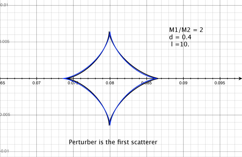
Figure 4: $M_{2}$ is the main lens at the origin: The “caustic curve” in blue is obtained by mapping the approximate critical curve using the approximate lens equation with the perturber as the first scatterer. The perturber is to the right on the real axis. The black “caustic curve” is from the same approximate critical curve mapped by the exact DSTP lens equation. The exact caustic curve of the DSTP lens (not shown) is hardly distinguishable from the black curve. The size of the caustic is $\approx 0.013$ in agreement with the analytic formula.

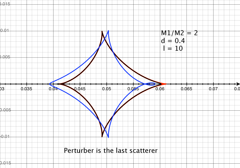
Figure 5: $M_{1}$ is the main lens at the origin: The “caustic curve” in blue is obtained by mapping the approximate critical curve using the approximate lens equation with the perturber as the last scatterer. The perturber is to the right on the real axis. The black “caustic curve” is from the same approximate critical curve mapped by the exact DSTP lens equation. The exact caustic caustic curve of the DSTP lens is shown in thick red. The slight difference of the black curve from the red curve can be discerned in the area around the real axis toward the perturber. The “caustic” sizes are $\approx 0.02$ in agreement with the analytic formula.

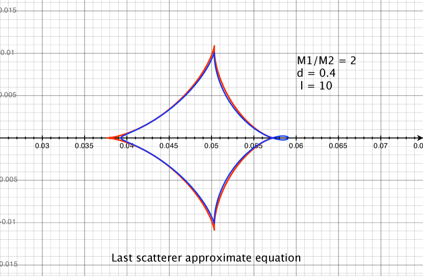
Figure 6: The “caustic curve” in blue is the same as in fig.5. The exact caustic curve of the approximate lens equation for the last scattering perturber is shown in red.

References

- Blandford and Narayan (1986) Blandford, R.D. and Narayan, N. 1986, ApJ 310, 568
- Erdl and Schneider (1993) Erdl, H. and Schneider, P. 1993, AA 268, 453
- Gavazzi et al (2008) Gavazzi, R., Treu, T., Koopmans, L. et al. 2008, ApJ, 677, 1046.
- Keeton (2003) Keeton, C.R. 2003, ApJ, 584, 664.
- Kochanek and Apostolakis (1986) Kochanek, C. and Apostolakis, J. 1986, MNRAS 235, 1073
- Petters (1997) Petters, A.O. 1997, J. Math. Phys., 38, 1605.
- Rhie (1999) Rhie, S.H. 1999, “Line Caustic Crossing and Limb Darkening”, arXiv:astro-ph/9912050.
- Rhie (2001) Rhie, S.H. 2001, “Can a Gravitational Quadruple Lens Produce 17 Images?”, arXiv:astro-ph/0103463.
- Rhie and Bennett (2010) Rhie, S. and Bennett, C. S. 2010, “Double Scattering Two Point Lenses and Three Image Rings”, arXiv.1000.0000[astro-ph].
- Werner et al (2008) Werner, M.C., An, J., Evans, N.W. 2008, MNRAS, 391, 668.