Detection of network inhomogeneity by total neighbor degree

Abstract

Inhomogeneity in networks can be detected by the analysis of the correlation of the total degree of nearest neighbors. This is illustrated by two models. The first one is a random multi-partitions network that the Aboav Weaire law, which predicts the linear relationship between the degree of node and the total degree of nearest neighbor, is being extended. The second one is a preferential attachment network with two partitions which shows scale free properties with power tail $\gamma$ within the range $2<\gamma\leq 3$. By plotting the total degree of neighbor verses the degree of each node in the networks, the scattered plot shows separable clustering as evidence for inhomogeneity in networks. The effectiveness of this new tool for the detection of inhomogeneity is demonstrated in real bipartite networks. By using this method, some interesting group of nodes of semantic and WWW networks have been found.

Keywords: network, degree inhomogeneity, neighbor degree correlation, modularity, bipartivity

1 Introduction

Many abstract structures and complex systems can be conveniently described by network. Examples include World Wide Web, power grid, food webs, word co-occurrence and protein interaction network [1, 2]. Depending on the system, some of them are naturally modeled as bipartite networks such as movie-actor network [2], paper coauthorship [3, 4], protein interaction [5], sexual relationship [6, 7], music sharing [8] and soccer championship [9]. One common tool to analyze a bipartite network is to project it into either set of nodes that are of interest to the specific investigation. In the projection, edges are usually reconnected as a complete subgraph [10, 11], possibly with some weighting schemes [12]. However, information is inevitably lost in any projection methods and even undesirable such as projecting sexual network into a female only or male only uni-partite network. Thus, some analyses have been carried out on the bipartite network directly [13, 14]. In general, a network with two partitions can have internal links and the resemblance with the bipartite network can be measured by bipartivity [15, 14]. In real world network, different type of nodes may not be known explicitly, so it is interesting to classify nodes into different groups [16]. A similar problem is community detection that focuses on classifying nodes into different partitions by optimizing modularity [17, 18].

The local environment of a node can be described by some typical properties such as degree and clustering coefficient. However, it is possible that the clustering coefficient is close to zero for a nearly bipartite network. In this case, the degree of the neighbors can therefore provide significant information. The degree-neighbor degree correlation can be characterized by the Pearson correlation coefficient [19] and it has been studied for networks with homogeneous neighbor degree by using the Aboav Weaire (AW) law [20, 21, 22]. The original works done by Aboav and Weaire in two-dimensional cellular networks have shown an empirically linear relationship between the averaged total neighbor degree and the node degree. Later, this law has been generalized for random, scale free and some real world networks [23]. The failure of this empirical observation thus provides a hint to detect local inhomogeneity of networks and possibly a method to group nodes together.

The aim of this paper is to study the correlation between total degree of nearest neighbors and the degree of the node itself for network with more than one partition. Through the extension of the AW law, we propose a simple method to classify nodes of nearly bipartite networks and modular networks. The rest of this paper is organized as follows: In section 2, we present a model of random multi-partition network and derive the generalization of the Aboav Weaire law of this network. In section 3, we study a preferential attachment network with two partitions and discuss the implication of this model to real world network. In section 4, we examine node degree and nearest neighbor degree correlation of real world networks for both bipartite networks and non-bipartite networks. The results suggest an interesting finding for the network of WordNet and WWW. Finally, a conclusion is given in section 5.

2 Multi-partitions random network

We begin our studies with a brief review of the Aboav-Weaire law. The AW law states that for a node with degree $k$ and mean neighbor degree $M(k)$, the averaged total neighbor degree has a linear relation with the node degree, given by $\left\langle kM(k)\right\rangle=Ak+B$, where $A$ and $B$ are the parameters depending on the network. For a random network with degree distribution $\mathcal{P}(k)$, the probability $\mathcal{Q}(k)$ of selecting one of the nearest neighbors with degree $k$ is proportional to the total degrees of all nodes with degree $k$, or $N\mathcal{P}(k)k$. Hence, after normalized, we get $\mathcal{Q}(k)=\mathcal{P}(k)k/\left\langle k\right\rangle$ [24] and the mean degree of neighbor is $\int\left(P(k)k/\left\langle k\right\rangle\right)kdk=\left\langle k^{2}\right\rangle/\left\langle k\right\rangle$. The Poisson degree distribution of random network gives $\left\langle k^{2}\right\rangle=\left\langle k\right\rangle^{2}-\left\langle k\right\rangle$ and so $A=\left\langle k\right\rangle+1$ [23]. In addition, the parameter $B$ represents the assortivity of a network and it takes value $B=0$.

Now, we consider a random network consists of $n$ different partitions that the inter-connections are specified between each partition. Formally, a random $n$-partition network with a set of nodes $V$ is composite by $n$ disjoint partition of nodes $\{V_{1},...,V_{n}\}$. For the network with size $|V|=N$, the size of each partition $V_{i}$ can be specified by the the fraction of nodes $r_{i}=|V_{i}|/N$ such that $\sum_{i}r_{i}=1$. The edge between each partition can be characterized by the probability matrix $\mathbf{P}=(p_{ij})$ that $p_{ij}$ represents the probability that any two nodes in $V_{i}$ and $V_{j}$, respectively, are connected. Hence, the diagonal entries represent the self-linkage probabilities and off-diagonal entries are the cross-linkage probabilities. For this model, the mean degree contribution from partition $V_{j}$ to $V_{i}$ is $p_{ij}r_{j}N$. By summing up all degree contribution from different partitions, we can get the mean degree for the partition $V_{i}$:

$$\left\langle k\right\rangle_{i}=\left(\sum_{j=1}^{n}p_{ij}r_{j}\right)N$$ (1)

where $\left\langle\cdot\right\rangle_{i}=\int\cdot\mathcal{P}_{i}(k)dk$ is the average taken over the degree distribution of partition $V_{i}$. Here, we consider the model with large $N$ limit such that the $N\gg p_{ij}N\gg 1$, so the probability distribution of each partition is close to a continuous Poisson distribution $\mathcal{P}(k)$ with the mean degree $\left\langle k\right\rangle_{i}$. Moreover, the mean degree $\left\langle k\right\rangle$ of the whole network is given by the weighted average of the mean degree of each partition, $\left\langle k\right\rangle=\sum_{i}r_{i}\left\langle k\right\rangle_{i}$.

The nearest neighbor degree distribution $\mathcal{Q}_{i}(k)$ is similar to the case of simple random network: a randomly selected neighbor located in partition $V_{j}$ gives degree distribution $\mathcal{P}_{j}(k)k/\left\langle k\right\rangle_{j}$. For a node $u$ in the partition $V_{i}$ with degree $k_{u}$, on average, there are $k_{u}(p_{ij}r_{j}N/\left\langle k\right\rangle_{i})$ edges connected to partition $V_{j}$. Therefore, the distribution $\mathcal{P}_{j}(k)k/\left\langle k\right\rangle_{j}$ of each partition has to be weighted by the factor which is proportional to $p_{ij}r_{j}$. After normalized, we have

$$\mathcal{Q}_{i}(k)=\frac{N}{\left\langle k\right\rangle_{i}}\sum_{j}p_{ij}r_{j}\frac{\mathcal{P}_{j}(k)k}{\left\langle k\right\rangle_{j}}$$ (2)

For this random network, it gives very good approximation because there is no strong degree correlation. The result is shown in Fig. 1a with the plot of a simulation result of $\mathcal{Q}_{i}(k)$ and the predicted result using the theoretical value of $\mathcal{P}_{j}(k)$ and $\left\langle k\right\rangle_{j}$.

For this model, the nodes in the same partition have homogeneous local environment. Hence, it is expected the linear relation of the total neighbor degree should still be hold for each partition separately, with the form $\left\langle kM(k)\right\rangle_{i}=A_{i}k+B_{i}$. For this random network, $B_{i}=0$ and the mean neighbor degree for the partition $V_{i}$ is

$$\left\langle M(k)\right\rangle_{i}=\frac{N}{\left\langle k\right\rangle_{i}}\sum_{j}p_{ij}r_{j}\frac{\left\langle k^{2}\right\rangle_{j}}{\left\langle k\right\rangle_{j}}$$ (3)

Therefore, the slope between the total neighbor degree and node degree is $A_{i}=\left\langle M(k)\right\rangle$. In Fig. 1b, the prediction using the above equation shows a good fit with the simulation result. Also, from the figure, it can be observed that the points for two partitions are separated into two clusters, while the degree distribution of both partition are collapsed together as shown in the inset of Fig. 1b. Hence, different type of nodes in the network can be revealed by the total neighbor degree. Note that the linear result is not valid for the whole network because this inhomogeneous local environment can only result in a non-linear curve, which is the superposition of two lines in the figure. Other than the nearly bipartite network, the clear separation is also hold for modular network with strong internal links because there can still have a large different in the degree between the internal nodes and external nodes.

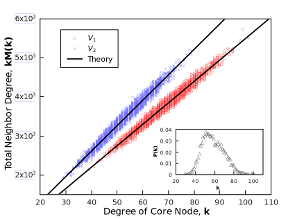
Figure 1: (a) The nearest neighbor degree distribution $\mathcal{Q}(k)$ of the random network with two partitions (b) Scattered plot of total neighbor degree $kM(k)$ vs $k$. $N=10000$, $r_{1}=0.4$, $p_{ii}=0.002$, $p_{12}=p_{21}=0.01$.

3 Preferential attachment network with two partitions

Most networks in real world exhibit scale free behavior that the degree distribution follows a power law at the high degree region. This property has been studied extensively and the representative model is the BA network introduced by Barabási and Albert [2] that is constructed by the mechanism of growth and preferential attachment. Here, we propose a model using similar mechanism together with different type of nodes labeled explicitly. In addition to the scale free property, the degree of nearest neighbor of this model exhibits a rich local behavior that the original BA model does not have.

Here, we focus on the study of two partitions network with growth and preferential attachment for simplicity. In this model, we can specify the ratio of node in each partition by $r_{i}$, such that $r_{1}+r_{2}=1$, and the number of edges added at each time step by a symmetric matrix $M=(m_{ij})$. We begin with a small network, such as a complete bipartite network or two nodes network with one edge. At each time step, one new node is added to the network, either belong to the partition $V_{1}$ with the probability $r_{1}$, or belong to the partition $V_{2}$ with probability $r_{2}$. In this grow process, the prescribed partition size ratio $r_{1}\approx|V_{1}|/N$ can be maintained. For every newly added node located at partition $V_{i}$, there are fixed number of edges $m_{ij}$ added between the new node and each partition $V_{j}$ in the network. A node with higher degree has higher chance to be connected, so for a old node $v$ located at partition $V_{j}$, the probability of being connected $\rho_{j}(k_{v})$ is linearly proportional to its own degree $k_{v}$. After normalized by the total degree of its own partition:

$$\rho_{j}(k_{v})=\frac{k_{v}}{\sum_{\alpha\in V_{j}}k_{\alpha}},\qquad\text{for }k_{v}\in V_{j}$$ (4)

After describing the model, we now look for the evolving of the degree of a given node $u$ in the partition $V_{1}$. Similar result for nodes in partition $V_{2}$ can be obtained by interchange the index 1 and 2. From the point of view of an old node $u$, it has, on average, $m_{11}\rho_{1}(k_{u})$ edges added for a new node in $V_{1}$ and $m_{12}\rho_{1}(k_{u})$ edges added for a new node in $V_{2}$. Hence, the change of degree for $u$ is given by the weighted sum of these two events:

$$k_{u}(t+1)-k_{u}(t)=r_{1}\left[m_{11}\rho_{1}(k_{u})\right]+r_{2}\left[m_{12}\rho_{1}(k_{u})\right]$$ (5)

The probability $\rho_{1}(k_{v})$ is evolving with time and the denominator depends on the the total degree of the partition $V_{1}$ given by:

$$\sum_{\alpha\in V_{1}}k_{\alpha}\approx(2r_{1}m_{11}+m_{12})t$$ (6)

where the first term is the average degree contribution for a node added to partition $V_{1}$ with probability $r_{1}$ and count $2m_{11}$ for each new node. The second term is the degree contribution from the cross link since both partitions gain $m_{12}=m_{21}$ degree for each new node. We can now adopt the continuum approach and write the evolution equation for the degree $k_{u}$:

$$\frac{\partial k_{u}(t)}{\partial t}=\left[\frac{r_{1}m_{11}+r_{2}m_{12}}{2r_{1}m_{11}+m_{12}}\right]\frac{k_{u}(t)}{t}$$ (7)

When a new node is added to the network at time $t_{i}$, it will have $m_{1}=m_{11}+m_{12}$ degree initially. Hence, the initial condition of the node $u$ is $k_{u}(t_{i})=m_{1}$ and so the evolving degree is:

$$k_{u}(t)=(t/t_{i})^{\frac{1}{\lambda_{1}}},\qquad\text{with }\lambda_{1}=\frac{2r_{1}m_{11}+m_{12}}{r_{1}m_{11}+r_{2}m_{12}}$$ (8)

The probability distribution of this partition $V_{1}$ is therefore given by:

$$\mathcal{P}_{1}(k)\sim\lambda_{1}m_{1}^{\lambda_{1}}k^{-\gamma_{1}}$$ (9)

where $\gamma_{1}=\lambda_{1}+1$ is the power of the tail of $\mathcal{P}_{1}(k)$. Similar result can also be obtained for the partition $V_{2}$. Hence, we obtain two degree distributions for two different partitions with power $\gamma_{1}$ and $\gamma_{2}$ respectively. One can verify that in the limiting case of $r_{2}=m_{12}=0$, the result reduced to the BA model with $\gamma_{1}=3$. Also, if the internal partition linkage $m_{ii}$ is strong for $i=1,2$, then $\gamma_{i}\approx 3$ for both partitions which is similar to the BA model because of the weak coupling between two partitions. By taking partial derivative on $\gamma_{i}$ with respect to different variables, it can be noted that the $\gamma_{i}$ is monotonic function for variables $r_{i}$ and $m_{ij}$ when $r_{i}\neq 0.5$. The implication of this result is that the power tail is $2<\gamma_{i}\leq 3$ for the region $0<r_{i}<0.5$ and $\gamma_{i}\geq 3$ for the region $0.5<r_{i}<1$. Comparing two degree distributions, the smaller partition has a slow decaying tail while the larger partition has a fast decaying tail as shown in the degree distribution in Fig. 2a.

Suppose we are now considering the degree distribution of the whole network, the slow decaying tail of one partition can dominate the high degree part so that only the tail with power $2<\gamma\leq 3$ can be observed, which is consistence with the measured power for most world networks [1]. In this model, $\gamma<3$ is the result of the existence of two classes of nodes and it implies that, by simply measuring degree distribution, nodes with different types cannot be distinguished. Hence, it is natural for us to ask whether some real networks have multiple classes of nodes that are yet to be unraveled. On the other hand, even though the degree distribution is scale free, this model suggests that the total nearest neighbor degree shows a different pattern for each partition.

From the above discussion, we know that the plotting of the total neighbor degree and the node degree is scattered into two branches. The result of a bipartite network without internal links is shown in Fig. 2b. To find the neighbor degree distribution and the slope $A_{i}$, one way is to use Eq. (2) and (3) by assuming the random connection: $p_{ii}=2m_{ii}/(Nr_{i})$ for $i=1,2$ and $p_{ij}=m_{ij}/(Nr_{i}r_{j})$ for $i\neq j$. For this bipartite network, the resulting neighbor degree distribution is good and the slope of total neighbor can be roughly approximated by $A_{1}\approx\left\langle k^{2}\right\rangle_{2}/\left\langle k\right\rangle_{2}$ and $A_{2}\approx\left\langle k^{2}\right\rangle_{1}/\left\langle k\right\rangle_{1}$ as shown by two straight lines in the figure. Nonetheless, when there are internal edges, the approximation of $A_{i}$ is not very good because the model with internal degree correlation cannot be treated as a simple random network. As shown in the inset of Fig. 2b, with existence of internal edges $m_{ii}=3$, the points fluctuate more widely than the simple bipartite network. In this case, as expected, the linear relation between degree and total neighbor degree for both partitions are less fit and points are deviated more from the lines. Therefore, the nodes for two partitions are partially mixed up and less distinguishable from each other at the low degree part.

The distinctive separation between two sets of nodes in Fig. 2b, especially at high degree or high total neighbor degree region, implies that these nodes can be easily classified into two groups. This two branches phenomenon does not occur for the BA model [23] in which the local environment is homogeneous for all nodes with the same degree. The points thus concentrate on a single line predicted by AW law, which show the result similar either branch in Fig. 2b. Hence, this phenomenon can be used to classify nodes into different partitions as we are introduced in the next section.

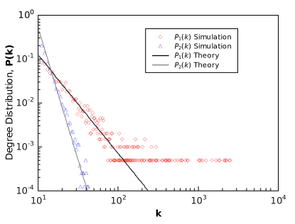
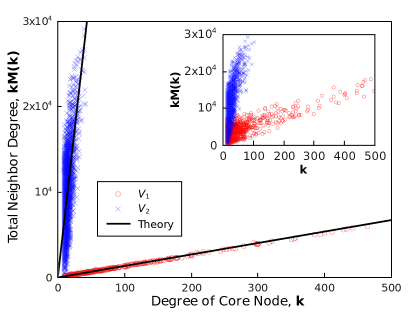
Figure 2: (a) Degree distribution $\mathcal{P}_{i}(k)$ for the partitions $V_{1}$ and $V_{2}$ of the scale free model with $N=10000$, $r_{1}=0.2$, $m_{ii}=0$, $m_{12}=10$ . (b) Scattered plot of total neighbor degree $kM(k)$ vs $k$. (inset) The corresponding network with some internal links $m_{ii}=3$.

4 Degree-Neighbor degree correlation in real world network

With the two models discussed in the previous section, we know that the total neighbor degree can be used to classify nodes. To test whether the branching phenomenon exists in real world network, we examine both explicitly bipartite and non-bipartite network. Undirected networks are used in the simulation and the results are shown below.

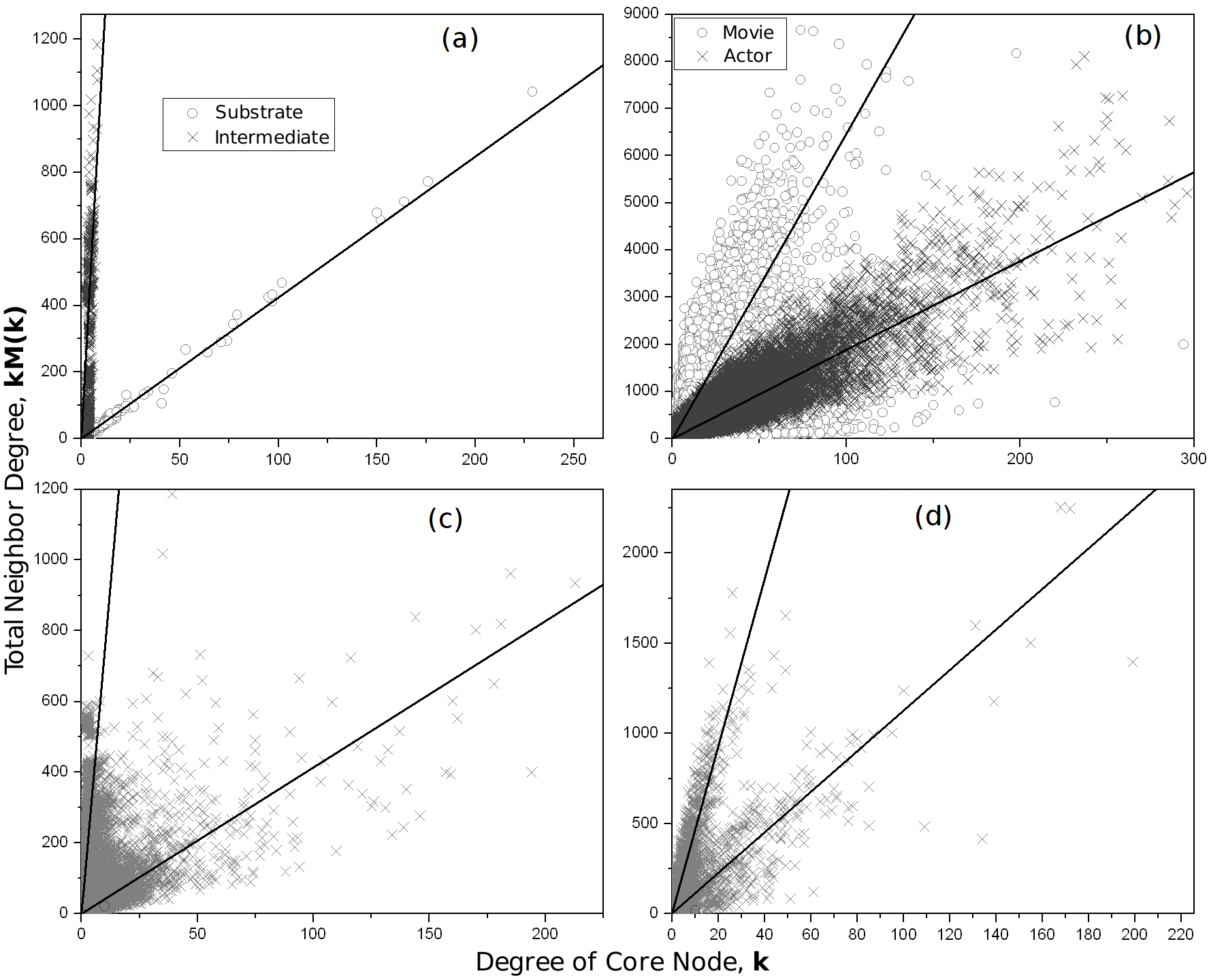
Figure 3: Scattered plot of total neighbor degree $kM(k)$ vs $k$, (a) the substrate and the intermediate in the metabolic network (E. Coli), (b) movies and actors in actor network, (c) WordNet, (d) California. The black lines are the fitting result of two branches.

The first example is metabolic networks [5] which are explicitly bipartite. It is an interaction network composed of the substrate and the intermediate complex. As shown in the Fig. 3a, the result of metabolic network is similar to the preferential attachment model we introduced and two branches are clearly identified. The substrate can have very high degree by its own nature so the tail part of the degree distribution of the whole network is dominated by power tail of substrate. In this case, the degree distribution of intermediate nodes is shadowed by the substrate nodes. However, in the scattered plot of the total neighbor degree, these two type of nodes are clearly separated into two clusters. Another bipartite network tested is the actor-movie network [2, 25] in which edges represent a particular actor playing in a particular movie. For this network, the degree distribution of both partitions is close to each other. So, it is expected that the points of the total neighbor degree for these two sets mixed at the region of low degree as shown in the Fig. 3b. Nevertheless, nodes can still be distinguished clearly other than the low degree region.

Examples discuss above are explicitly bipartite so, in some sense, they should be easily distinguishable. However, it is a challenge to classified nodes into different groups for networks without having any a prior knowledge on their origins. Now, similar method can be employed to classify nodes by detecting the local inhomogeneity and the branching in the total neighbor degree. One of the examples in this category is the semantic network of the WordNet project [26] which studies the semantic relationship between different English words. As shown in Fig. 3c, two branches for this network can be observed. Through the inspection of words in the network, it can be concluded that the steeper branch contains words that are specialized while the other branch corresponds to the generic words. Even though specialized words have low degree, they can still have high total neighbor degree because they are typically connected to generic words that have high degree. Another one is the California web subgraph networks [27, 28]. It is constructed by linking webpages together depending on the querying results of search engine. It is not an explicitly bipartite network, but two different branches is clearly shown in the Fig. 3d.

Table 1: Results of two lines fitting for different networks. $N_{1}$ and $N_{2}$ are the number of nodes classified into the corresponding partitions by this method. $c$ is the ratio of number of correctly classified nodes divided by total number nodes in the network.

Network	$s_{1}$	$s_{2}$	$N_{1}$	$N_{2}$	$c$
Random network in Fig. 1a	55.3	65.4	4038	5962	1.00
Scale free network in Fig. 2b	13.3	746	1942	8058	1.00
Scale free network in inset of Fig. 2b	27.6	363	2013	7987	0.85
Metabolic E. Coli [5]	4.24	106	766	1509	0.92
Actor-movie [2]	18.8	64.7	383640	127823	0.57
WordNet network [26]	4.14	75.0	34652	42191	-
California subnetwork [27]	11.2	46.4	2266	3909	-

To quantify the observation, we perform a least square fit to find the best fitting lines and group nodes together. For a simple homogeneous network, the Aboav-Weaire law predicts that the data point of average total neighbor degree verse degree will fit into one single line. Thus, for a network with two different partitions, we expect that there should be two clear straight lines. With the same reason discussed for the random $n$-partition network, the $y$-intercept is usually small and we assume it to be zero. Hence, we look for the lines of the form $y=s_{1}x$ and $y=s_{2}x$, with the slopes $s_{1}$ and $s_{2}$ as the fitting parameters, such that the square of distance between different points to the two lines is minimized:

$$E(s_{1},s_{2})=\sum_{i=1}^{N}\min\left(\frac{(y_{i}-s_{1}x_{i})^{2}}{1+s_{1}^{2}},\frac{(y_{i}-s_{2}x_{i})^{2}}{1+s_{2}^{2}}\right)$$ (10)

Here, we can get the best fitting slopes $s_{1}$ and $s_{2}$ by minimized $E(s_{1},s_{2})$. This method provides a simple classification of nodes into two groups. If a network is homogeneous for the local environment, then there may be only one group of nodes and the resulting $s_{1}$ and $s_{2}$ should take a value close to each other. The corresponding fitting results are plotted as two black straight lines in the Fig. 3. Moreover, the fitting and classification results is shown in Table 1 for networks used in this paper. From the table, we can see that the classification is very good for the models we studied, even for the preferential attachment network with internal linkages. For the real world bipartite networks, we can see that the classification is acceptable for the metabolic network and the actor-movie network. For the non-bipartite network, the fitting curves represent those two branches very good in Fig. 3. In addition, the large different in the values of $s_{1}$ and $s_{2}$ signify that these networks are better be described by two branches and so we can classify them into two groups.

5 Summary

In sum, we have studied nearest neighbor degree correlation for the random multi-partition network, preferential attachment network and some real world networks. Through the analysis of the extended AW law, the exact neighbor degree distribution is computed for random multi-partition network. Furthermore, we show that there is a linear relationship between total neighbor degree and the node degree for each partition separately, but not linear for the whole network. This phenomenon is especially distinct for the preferential attachment network which also model the scale free property with $2<\gamma\leq 3$. The clustering of points in the scattered plot of total neighbor degree verse degree therefore suggests a way to classify node into different groups. By applying this classification scheme to the models studied and real bipartite networks, we show that the grouping of node is satisfactory. We also find an interesting subset of nodes in the WordNet and California subgraph networks which are not bipartite.

References

- [1] R. Albert and A. L. Barabási. Statistical mechanics of complex networks. Rev. Mod. Phys., 74:47–97, 2002.
- [2] A. L. Barabási and R. Albert. Emergence of scaling in random networks. Science, 286:509–512, 1999.
- [3] M. E. J. Newman. Scientific collaboration networks. i. network construction and fundamental results. Phys. Rev. E, 64:016131, 2001.
- [4] M. E. J. Newman and M. Girvan. Finding and evaluating community structure in networks. Phys. Rev. E, 69:026113, 2004.
- [5] H. Jeong, B. Tombor, R. Albert, Z. N. Oltvai, and A.-L. Barabasi. The large-scale organization of metabolic networks. Nature, 407:651–654, 2000.
- [6] F. Liljeros, C.R. Edling, L.A.N. Amaral, H.E. Stanley, and Y. Aberg. The web of human sexual contacts. Nature, 411:907–908, 2001.
- [7] P. S. Bearman, J. Moody, and K. Stovel. Chains of affection: The structure of adolescent romantic and sexual networks. American Journal of Sociology, 110:44–91, 2004.
- [8] R. Lambiotte and M. Ausloos. Uncovering collective listening habits and music genres in bipartite networks. Phys. Rev. E, 72:066107, 2005.
- [9] R. N. Onody and P. A. de Castro. Complex network study of brazilian soccer players. Phys. Rev. E, 70:037103, 2004.
- [10] M. E. J. Newman. Properties of highly clustered networks. Phys. Rev. E, 68:026121, 2003.
- [11] M. E. J. Newman. Coauthorship networks and patterns of scientific collaboration. Proc. Natl. Acad. Sci. U. S. A., 101:5200–5205, 2004.
- [12] T. Zhou, J. Ren, M. Medo, and Y. C. Zhang. Bipartite network projection and personal recommendation. Phys. Rev. E, 76:046115, 2007.
- [13] T. S. Evans and A. D. K. Plato. Exact solution for the time evolution of network rewiring models. Phys. Rev. E, 75:056101, 2007.
- [14] P. Holme, F. Liljeros, C. R. Edling, and B. J. Kim. Network bipartivity. Phys. Rev. E, 68:056107, 2003.
- [15] E. Estrada and J. A. Rodríguez-Velázquez. Spectral measures of bipartivity in complex networks. Phys. Rev. E, 72:046105, 2005.
- [16] J. L. Guillaume and M. Latapy. Bipartite graphs as models of complex networks. Physica A, 371:795 – 813, 2006.
- [17] M. J. Barber. Modularity and community detection in bipartite networks. Phys. Rev. E, 76:066102, 2007.
- [18] J. Reichardt and S. Bornholdt. Statistical mechanics of community detection. Phys. Rev. E, 74:016110, 2006.
- [19] M. E. J. Newman. Assortative mixing in networks. Phys. Rev. Lett., 89:208701, 2002.
- [20] D. A. Aboav. The arrangement of grains in a polycrystal. Metallography, 3:383 – 390, 1970.
- [21] D. Weaire. Some remarks on the arrangement of grains in a polycrystal. Metallography, 7:157 – 160, 1974.
- [22] D. A. Aboav. The arrangement of cells in a net. Metallography, 13:43 – 58, 1980.
- [23] C. W. Ma and K. Y. Szeto. Linear relation on the correlation in complex networks. Phys. Rev. E, 73:047101, 2006.
- [24] M. E. J. Newman, S. H. Strogatz, and D. J. Watts. Random graphs with arbitrary degree distributions and their applications. Phys. Rev. E, 64:026118, 2001.
- [25] R. Albert, H. Jeong, and A. L. Barabási. Internet: Diameter of the world-wide web. Nature, 401:130–131, 1999.
- [26] WordNet, http://wordnet.princeton.edu/.
- [27] J. Kleinberg. Proc. 9th ACM-SIAM Symposium on Discrete Algorithms, 1998.
- [28] http://www.cs.cornell.edu/courses/cs685/2002fa/.