Cooperative Feedback for Multi-Antenna Cognitive Radio Networks

Abstract

Cognitive beamforming (CB) is a multi-antenna technique for efficient spectrum sharing between primary users (PUs) and secondary users (SUs) in a cognitive radio network. Specifically, a multi-antenna SU transmitter applies CB to suppress the interference to the PU receivers as well as enhance the corresponding SU-link performance. In this paper, for a multiple-input-single-output (MISO) SU channel coexisting with a single-input-single-output (SISO) PU channel, we propose a new and practical paradigm for designing CB based on the finite-rate cooperative feedback from the PU receiver to the SU transmitter. Specifically, the PU receiver communicates to the SU transmitter the quantized SU-to-PU channel direction information (CDI) for computing the SU transmit beamformer, and the interference power control (IPC) signal that regulates the SU transmission power according to the tolerable interference margin at the PU receiver. Two CB algorithms based on cooperative feedback are proposed: one restricts the SU transmit beamformer to be orthogonal to the quantized SU-to-PU channel direction and the other relaxes such a constraint. In addition, cooperative feedforward of the SU CDI from the SU transmitter to the PU receiver is exploited to allow more efficient cooperative feedback. The outage probabilities of the SU link for different CB and cooperative feedback/feedforward algorithms are analyzed, from which the optimal bit-allocation tradeoff between the CDI and IPC feedback is characterized.

I Introduction

In a cognitive radio network, secondary users (SUs) are allowed to access the spectrum allocated to a primary network so long as the resultant interference to the primary users (PUs) is within a tolerable margin [1]. Cognitive beamforming (CB) is a promising technique that enables a multi-antenna SU transmitter to regulate its interference to each PU receiver by intelligent beamforming, and thereby transmit more frequently with larger power with respect to a single-antenna SU transmitter. The optimal CB requires the SU transmitter to acquire the channel state information (CSI) of its interference channels to the PU receivers and even that of the primary links, which is difficult without the PUs’ cooperation. We consider a two-user cognitive-radio network comprising a multiple-input-single-output (MISO) SU link and a single-input-single-output (SISO) PU link. This paper establishes a new approach of enabling CB at the SU transmitter based on the finite-rate CSI feedback from the PU receivers and presents a set of jointly designed CB and feedback algorithms. The effect of feedback CSI quantization on the SU link performance is quantified, yielding insight into the feedback requirement.

Existing CB designs assume that the SU transmitter either has prior CSI of the interference channels to the PU receivers or can acquire such information by observing the PU transmissions, which may be impractical. Assuming perfect CSI of the SU-to-PU channels, the optimal CB design is proposed in [2] for maximizing the SU throughput subject to a given set of interference power constraints at the PU receivers. The perfect CSI assumption is relaxed in [3] and a more practical CB algorithm is designed where a SU transmitter estimates the required CSI by exploiting channel reciprocity and periodically observing the PU transmissions. However, channel estimation errors can cause unacceptable residual interference from the SU transmitter to the PU receivers. This issue is addressed in [4] by optimizing the cognitive beamfomer to cope with CSI inaccuracy. Besides CB, the power of the SU transmitter can be adjusted opportunistically to further increase the SU throughput by exploiting the primary-link CSI as proposed in [5] and [6]. Such CSI, however, is even more difficult for the SU to obtain than that of the SU-to-PU channels if the PU receivers provide no feedback.

For multiple-input multiple-output (MIMO) wireless systems, CSI feedback from the receiver enables precoding at the transmitter, which not only enhances the throughput but also simplifies the transceiver design [7]. However, CSI feedback can incur substantial overhead due to the multiplicity of MIMO channel coefficients. This motivates active research on designing efficient feedback quantization algorithms, called limited feedback [8]. There exists a rich literature on limited feedback [9] where MIMO CSI quantizers have been designed based on various principles such as line packing [10] and Lloyd’s algorithm [11], and targeting different systems ranging from single-user beamforming [12, 10] to multiuser downlink [13, 14, 15]. In view of prior work, limited feedback for coexisting networks remains a largely uncharted area. In particular, there exist few results on limited feedback for cognitive radio networks.

In traditional cognitive radio networks, primary users have higher priority of accessing the radio spectrum and are reluctant to cooperate with secondary users having lower priority and belonging to an alien network [16]. However, inter-network cooperation is expected in the emerging heterogeneous wireless networks that employ macro-cells, micro-cells, and femto-cells to serve users with different priorities [17]. For instance, a macro-cell mobile user can assist the cognitive transmission in a nearby femto-cell. Thus, the design of efficient cooperation methods in cognitive radio networks will facilitate the implementation of next-generation heterogeneous wireless networks.

This paper presents a new and practical paradigm for designing CB based on the finite-rate CSI feedback from the PU receiver to the SU transmitter, called cooperative feedback. To be specific, the PU receiver communicates to the SU transmitter i) the channel-direction information (CDI), namely the quantized shape of the SU-to-PU MISO channel, for computing the cognitive beamformer and ii) the interference-power-control (IPC) signal that regulates the SU transmission power according to the tolerable interference margin at the PU receiver. Our main contributions are summarized as follows.

1. We present two CB algorithms for the SU transmitter based on the finite-rate cooperative feedback from the PU receiver. One is orthogonal cognitive beamforming (OCB) where the SU transmit beamformer is restricted to be orthogonal to the feedback SU-to-PU channel shape and the SU transmission power is controlled by the IPC feedback. The other is non-orthogonal cognitive beamforming (NOCB) for which the orthogonality constraint on OCB is relaxed and the matching IPC signal is designed.

2. In addition to cooperative feedback, we propose cooperative feedforward of the secondary-link CSI from the SU transmitter to the PU receiver. The feedforward is found to enable more efficient IPC feedback, allowing larger SU transmission power.

3. We analyze the secondary-link performance in terms of the signal-to-noise ratio (SNR) outage probability for OCB. In particular, regardless of whether there is feedforward, the SU outage probability is shown to be lower-bounded in the high SNR regime due to feedback CDI quantization. The lower bound is proved to decrease exponentially with the number of CDI feedback bits.

4. Finally, we derive the optimal bit allocation for the CDI and IPC feedback under a sum feedback rate constraint, which minimizes an upper bound on the SU outage probability.

The remainder of this paper is organized as follows. Section II introduces the system model. Section III presents the jointly designed CB and cooperative feedback algorithms. Section IV and Section V provide the analysis of the SU outage probability and the optimal tradeoff between the CDI and IPC feedback-bit allocation, respectively. Simulation results are given in Section VI, followed by concluding remarks in Section VII.

II System Model

We consider a primary link coexisting with a secondary link. The transmitter $\mathsf{T_{\mathsf{p}}}$ and the receiver $\mathsf{R_{\mathsf{p}}}$ of the primary link both have a single antenna, while the secondary link comprises a multi-antenna transmitter $\mathsf{T_{\mathsf{s}}}$ and a single-antenna receiver $\mathsf{R_{\mathsf{s}}}$. The multiple antennas at $\mathsf{T_{\mathsf{s}}}$ are employed for beamforming where the beamformer is represented by ${\mathbf{f}}$. All channels follow independent block fading. The channel coefficients of the primary and secondary links are independent and identically distributed (i.i.d.) circularly symmetric complex Gaussian random variables with zero-mean and unit-variance, denoted by $\mathcal{CN}(0,1)$. Consequently, the primary signal received at $\mathsf{R_{\mathsf{p}}}$ has the power $P_{\mathsf{p}}g_{\mathsf{p}}$, where $P_{\mathsf{p}}=\|{\mathbf{f}}\|^{2}$ is the transmission power of $\mathsf{T_{\mathsf{p}}}$ and $g_{\mathsf{p}}$ the primary channel power that is exponentially distributed with unit variance, denoted by $\exp(1)$. The MISO channels from $\mathsf{T_{\mathsf{s}}}$ to $\mathsf{R_{\mathsf{p}}}$ and from $\mathsf{T_{\mathsf{s}}}$ to $\mathsf{R_{\mathsf{s}}}$ are represented by the $L\times 1$ vectors ${\mathbf{h}}_{\textsf{x}}$ consisting of i.i.d. $\mathcal{CN}(0,1)$ elements and ${\mathbf{h}}_{\mathsf{s}}$ comprising i.i.d. $\mathcal{CN}(0,\lambda)$ elements, respectively, where $0<\lambda<1$ accounts for a larger path loss between $\mathsf{T_{\mathsf{s}}}$ and $\mathsf{R_{\mathsf{p}}}$ than that between $\mathsf{T_{\mathsf{s}}}$ and $\mathsf{R_{\mathsf{s}}}$ (or between $\mathsf{T_{\mathsf{p}}}$ and $\mathsf{R_{\mathsf{p}}}$). To facilitate analysis, ${\mathbf{h}}_{\textsf{x}}$ is decomposed into the channel gain $g_{\textsf{x}}=\|{\mathbf{h}}_{\textsf{x}}\|^{2}/\lambda$ and channel shape ${\mathbf{s}}_{\textsf{x}}={\mathbf{h}}_{\textsf{x}}/\|{\mathbf{h}}_{\textsf{x}}\|$, and hence ${\mathbf{h}}_{\textsf{x}}=\sqrt{\lambda g_{\textsf{x}}}{\mathbf{s}}_{\textsf{x}}$; similarly, let ${\mathbf{h}}_{\mathsf{s}}=\sqrt{g_{\mathsf{s}}}{\mathbf{s}}_{\mathsf{s}}$. The channel power $g_{\textsf{x}}$ and $g_{\mathsf{s}}$ follow independent chi-square distributions with $L$ complex degrees of freedom.

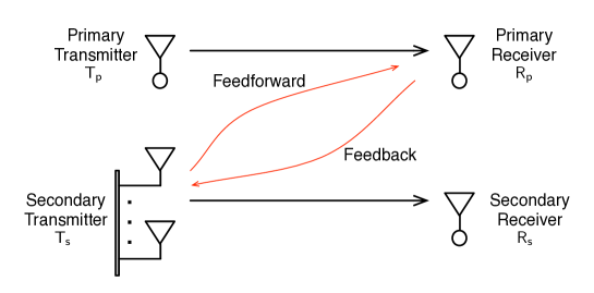
Figure 1: Coexisting single-antenna primary and multi-antenna secondary links

The primary receiver $\mathsf{R_{\mathsf{p}}}$ cooperates with the secondary transmitter $\mathsf{T_{\mathsf{s}}}$ to maximize the secondary-link throughput without compromising the primary-link performance. We assume that $\mathsf{R_{\mathsf{p}}}$ estimates ${\mathbf{h}}_{\textsf{x}}$ and $g_{\mathsf{p}}$ perfectly and has prior knowledge of the maximum SU transmission power $P_{\max}$. This enables $\mathsf{R_{\mathsf{p}}}$ to compute and communicate to $\mathsf{T_{\mathsf{s}}}$ the IPC signal and the CDI ${\mathbf{s}}_{\textsf{x}}$. Under a finite-rate feedback constraint, the IPC and CDI feedback must be both quantized. Let $\hat{{\mathbf{s}}}_{\textsf{x}}$ denote the output of quantizing ${\mathbf{s}}_{\textsf{x}}$. Following [18, 19], we adopt the quantization model where $\hat{{\mathbf{s}}}_{\textsf{x}}$ lies on a hyper sphere-cap centered at ${\mathbf{s}}_{\textsf{x}}$ and its radius depends on the quantization resolution. Specifically, the quantization error $\epsilon=1-|\hat{{\mathbf{s}}}_{\textsf{x}}^{\dagger}{\mathbf{s}}_{\textsf{x}}|^{2}$ has the following cumulative distribution function for $L>1$ [18]

$$\Pr(\epsilon\leq\tau)=\left\{\begin{aligned} &2^{B}\tau^{L-1},&&0\leq\tau\leq 2^{-\frac{B}{L-1}}\\ &1,&&\textrm{otherwise}\end{aligned}\right.$$ (1)

where $B$ is the number of CDI feedback bits. The IPC feedback quantization is discussed in Section III.

Feedback of ${\mathbf{s}}_{\mathsf{s}}$ from $\mathsf{R_{\mathsf{s}}}$ to $\mathsf{T_{\mathsf{s}}}$ is also required for computing the beamformer ${\mathbf{f}}$, called local feedback. We assume no feedback of $g_{\mathsf{s}}$ from $\mathsf{R_{\mathsf{s}}}$ to $\mathsf{T_{\mathsf{s}}}$. Thus the transmission power $P_{\mathsf{s}}$ of $\mathsf{T_{\mathsf{s}}}$ is independent of $g_{\mathsf{s}}$. We also consider the scenario where $\mathsf{T_{\mathsf{s}}}$ sends ${\mathbf{s}}_{\mathsf{s}}$ to $\mathsf{R_{\mathsf{p}}}$, called feedforward, prior to cooperative feedback. This information is used by $\mathsf{R_{\mathsf{p}}}$ to predict the beamformer at $\mathsf{T_{\mathsf{s}}}$ and thereby tolerate larger transmission power at $\mathsf{T_{\mathsf{s}}}$. For simplicity, the local feedback and the feedforward are assumed perfect. This assumption allows us to focus on the effect of finite-rate cooperative feedback.

The performance of the primary and secondary links are both measured by the SNR or signal-to-interference-plus-noise ratio (SINR) outage probability. Accordingly, the data rates for the primary and secondary links are fixed as $R_{\mathsf{p}}=\log_{2}(1+\theta_{\mathsf{p}})$ and $R_{\mathsf{s}}=\log_{2}(1+\theta_{\mathsf{s}})$, respectively, where $\theta_{\mathsf{p}}$ and $\theta_{\mathsf{s}}$ specify the receive SNR/SINR thresholds for correct decoding. The receive SNR and SINR at $\mathsf{R_{\mathsf{p}}}$ are given by

$$\mathsf{SNR}_{\mathsf{p}}=\gamma_{\mathsf{p}}g_{\mathsf{p}}\quad\textrm{and}\quad\mathsf{SINR}_{\mathsf{p}}=\frac{\gamma_{\mathsf{p}}g_{\mathsf{p}}}{1+\frac{\lambda g_{\textsf{x}}}{\sigma^{2}}|{\mathbf{f}}^{\dagger}{\mathbf{s}}_{\textsf{x}}|^{2}}$$ (2)

where $\gamma_{\mathsf{p}}$ is the PU transmit SNR given by $\gamma_{\mathsf{p}}=P_{\mathsf{p}}/\sigma^{2}$, and the noise samples at both $\mathsf{R_{\mathsf{p}}}$ and $\mathsf{R_{\mathsf{s}}}$ are i.i.d. $\mathcal{CN}(0,\sigma^{2})$ random variables. The PU outage probability is unaffected by the SU transmission and can be written as

$$\bar{P}_{\textrm{out}} = \Pr(\mathsf{SINR}_{\mathsf{p}}<\theta_{\mathsf{p}})$$ (3)

$$= \Pr(\mathsf{SNR}_{\mathsf{p}}<\theta_{\mathsf{p}})$$

$$= 1-e^{-\frac{\theta_{\mathsf{p}}}{\gamma_{\mathsf{p}}}}$$ (4)

where the equality in (3) specifies a constraint on the SU CB design and (4) follows from that the primary channel gain $g_{\mathsf{p}}$ is distributed as $\exp(1)$. In a heterogeneous network, a primary transmitter such as a macro-cell base station is located far away from a receiver served by a secondary transmitter such as a femto-cell base station. Therefore, interference from $\mathsf{T_{\mathsf{p}}}$ to $\mathsf{R_{\mathsf{s}}}$ is assumed negligible and the receive SNR at $\mathsf{R_{\mathsf{s}}}$ is

$$\mathsf{SNR}_{\mathsf{s}}=\frac{g_{\mathsf{s}}}{\sigma^{2}}|{\mathbf{f}}^{\dagger}{\mathbf{s}}_{\mathsf{s}}|^{2}.$$ (5)

It follows that the SU outage probability is

$$P_{\mathsf{out}}=\Pr(\mathsf{SNR}_{\mathsf{s}}\leq\theta_{\mathsf{p}}).$$ (6)

III Cognitive Beamforming and Cooperative Feedback Algorithms

The beamforming algorithms are designed to minimize the secondary link outage probability under the PU-outage-probability constraint in (3). The OCB and NOCB algorithms together with matching IPC feedback designs are discussed in separate subsections.

III-A Orthogonal Cognitive Beamforming

The OCB beamformer at $\mathsf{T_{\mathsf{s}}}$, denoted as ${\mathbf{f}}_{\mathsf{o}}$, suppresses interference to $\mathsf{R_{\mathsf{p}}}$ and yet enhances $\mathsf{SNR}_{\mathsf{s}}$ in (5). To this end, ${\mathbf{f}}_{\mathsf{o}}$ is constrained to be orthogonal to the feedback CDI $\hat{{\mathbf{s}}}_{\textsf{x}}$, giving the name OCB. Despite the orthogonality constraint, there exists residual interference from $\mathsf{T_{\mathsf{s}}}$ to $\mathsf{R_{\mathsf{p}}}$ due to the quantization error in $\hat{{\mathbf{s}}}_{\textsf{x}}$. The interference power can be controlled to satisfy the constraint in (3) using IPC feedback from $\mathsf{R_{\mathsf{p}}}$ to $\mathsf{T_{\mathsf{s}}}$. Specifically, the transmission power of $\mathsf{T_{\mathsf{s}}}$, defined as $P_{\mathsf{s}}=\|{\mathbf{f}}_{\mathsf{o}}\|^{2}$, satisfies the constraint $P_{\mathsf{s}}\leq\hat{\eta}$, where $\hat{\eta}$ is the quantized IPC feedback signal to be designed in the sequel. It follows from above discussion that the beamformer ${\mathbf{f}}_{\mathsf{o}}$ solves the following optimization problem

maximize: $$|{\mathbf{f}}_{\mathsf{o}}^{\dagger}{\mathbf{s}}_{\mathsf{s}}|^{2}$$ (7)

subject to: $${\mathbf{f}}_{\mathsf{o}}^{\dagger}\hat{{\mathbf{s}}}_{\textsf{x}}=0$$

$$\|{\mathbf{f}}_{\mathsf{o}}\|^{2}\leq\hat{\eta}.$$

To solve the above problem, we decompose ${\mathbf{s}}_{\mathsf{s}}$ as ${\mathbf{s}}_{\mathsf{s}}=a\hat{{\mathbf{s}}}_{\textsf{x}}+b\hat{{\mathbf{s}}}_{\perp}$ where $\hat{{\mathbf{s}}}_{\perp}$ is an $L\times 1$ vector with unit norm such that $\hat{{\mathbf{s}}}_{\perp}^{\dagger}\hat{{\mathbf{s}}}_{\textsf{x}}=0$, and the coefficients $(a,b)$ satisfy $|a|^{2}+|b|^{2}=1$. With this decomposition, the optimization problem in (7) can be rewritten as

maximize: $$|b{\mathbf{f}}_{\mathsf{o}}^{\dagger}\hat{{\mathbf{s}}}_{\perp}|^{2}$$ (8)

subject to: $$\|{\mathbf{f}}_{\mathsf{o}}\|^{2}\leq\hat{\eta}.$$

It follows that ${\mathbf{f}}_{\mathsf{o}}$ implements the maximum-ratio transmission [20] and is thus given as

$${\mathbf{f}}_{\mathsf{o}}=\sqrt{\hat{\eta}}\hat{{\mathbf{s}}}_{\perp}.$$ (9)

III-A1 The Design of IPC Feedback

The unquantized IPC feedback signal, denoted as $\eta$, is designed such that the constraint $\|{\mathbf{v}}\|^{2}\leq\eta$ is sufficient for enforcing that in (3). The quantization of $\eta$ will be discussed in the next subsection. The constraint in (3) can be translated into one on the residual interference power $I_{\mathsf{o}}$ from $\mathsf{T_{\mathsf{s}}}$ to $\mathsf{R_{\mathsf{p}}}$ as follows. Let $\mathsf{null}(\hat{{\mathbf{s}}}_{\textsf{x}})$ denote the null space of $\hat{{\mathbf{s}}}_{\textsf{x}}$ and its basis vectors are represented as $({\mathbf{e}}_{1},{\mathbf{e}}_{2},\cdots,{\mathbf{e}}_{L-1})$. It follows from the CDI quantization model in Section II that

$$\sum_{n=1}^{L-1}|{\mathbf{s}}_{\textsf{x}}^{\dagger}{\mathbf{e}}_{n}|^{2}=\epsilon.$$ (10)

Without loss of generality, let ${\mathbf{e}}_{1}=\hat{{\mathbf{s}}}_{\perp}$ since $\hat{{\mathbf{s}}}_{\perp}\in\mathsf{null}(\hat{{\mathbf{s}}}_{\textsf{x}})$ and define $\delta=|{\mathbf{s}}_{\textsf{x}}^{\dagger}\hat{{\mathbf{s}}}_{\perp}|^{2}$. Thus from (10) and since $|{\mathbf{s}}_{\textsf{x}}^{\dagger}\hat{{\mathbf{s}}}_{\perp}|^{2}\leq\sum_{n=1}^{L-1}|{\mathbf{s}}_{\textsf{x}}^{\dagger}{\mathbf{e}}_{n}|^{2}$, we can obtain that $\delta\leq\epsilon$. Furthermore, define ${\mathbf{q}}=\sum_{n=2}^{L-1}({\mathbf{s}}_{\textsf{x}}^{\dagger}{\mathbf{e}}_{n}){\mathbf{e}}_{n}$ and ${\mathbf{s}}_{\textsf{x}}$ can be decomposed as

$${\mathbf{s}}_{\textsf{x}}=e^{j\theta_{1}}\sqrt{1-\epsilon}\hat{{\mathbf{s}}}_{\textsf{x}}+e^{j\theta_{2}}\sqrt{\delta}\hat{{\mathbf{s}}}_{\perp}+{\mathbf{q}}$$ (11)

where the angles $(\theta_{1},\theta_{2})$ represent appropriate phase rotations. Using the above expression, $I_{\mathsf{o}}$ can be upper-bounded as

$$I_{\mathsf{o}} = \lambda g_{\textsf{x}}|{\mathbf{f}}^{\dagger}{\mathbf{s}}_{\textsf{x}}|^{2}$$ (12)

$$= \lambda g_{\textsf{x}}|\sqrt{\eta}\hat{{\mathbf{s}}}_{\perp}^{\dagger}(e^{j\theta_{1}}\sqrt{1-\epsilon}\hat{{\mathbf{s}}}_{\textsf{x}}+e^{j\theta_{2}}\sqrt{\delta}\hat{{\mathbf{s}}}_{\perp}+{\mathbf{q}})|^{2}$$ (13)

$$= \lambda g_{\textsf{x}}\eta\delta$$ (14)

$$\leq \lambda g_{\textsf{x}}\eta\epsilon$$ (15)

where (13) is obtained by substituting (9) and (11). Note that computing $\delta$ at $\mathsf{R_{\mathsf{p}}}$ requires $\hat{{\mathbf{s}}}_{\perp}$ that can be derived from the feedforward of ${\mathbf{s}}_{\mathsf{s}}$ from $\mathsf{T_{\mathsf{s}}}$. Therefore, $I_{\mathsf{o}}$ can be obtained at $\mathsf{R_{\mathsf{p}}}$ using (14) for the case of feedforward or otherwise approximated using (15). Based on the principle of opportunistic power control in [5], the constraint in (3) is equivalent to that:

$$I_{\mathsf{o}}\leq\omega,\quad\textrm{if}\ \omega\geq 0$$ (16)

where

$$\omega=\sigma^{2}\left(\frac{\gamma_{\mathsf{p}}g_{\mathsf{p}}}{\theta_{\mathsf{p}}}-1\right).$$ (17)

If $\omega<0$, $I_{\mathsf{o}}$ can be arbitrarily large since $\mathsf{R_{\mathsf{p}}}$ experiences outage even without any interference from $\mathsf{T_{\mathsf{s}}}$. For the case without feedforward, the IPC signal $\eta$ is obtained by combining (15) and (16) as

$$\eta=\left\{\begin{aligned} &\frac{\omega}{\lambda g_{\textsf{x}}\epsilon},&&\omega\geq 0\\ &P_{\max},&&\textrm{otherwise}.\end{aligned}\right.$$ (18)

The counterpart of $\eta$ for the case of feedforward, denoted as $\acute{\eta}$, follows from (14) and (16) as

$$\acute{\eta}=\left\{\begin{aligned} &\frac{\omega}{\lambda g_{\textsf{x}}\delta},&&\omega\geq 0\\ &P_{\max},&&\textrm{otherwise}.\end{aligned}\right.$$ (19)

Note that the constraint $P_{\mathsf{s}}\leq\acute{\eta}$ is looser than $P_{\mathsf{s}}\leq\eta$ in the case of $w\geq 0$ since $\delta\leq\epsilon$.

III-A2 The Quantization of IPC Feedback

Let $\hat{\eta}$ denote the $(A+1)$-bit output of quantizing $\eta$. The first bit indicates whether there is an outage event at $\mathsf{R_{\mathsf{p}}}$; the following $A$ bits represent $\hat{\eta}$ if $\mathsf{R_{\mathsf{p}}}$ is not in outage (i.e., $\omega\geq 0$) or otherwise are neglected by $\mathsf{T_{\mathsf{s}}}$. Given $\omega\geq 0$, $\hat{\eta}$ is constrained to take on values from a finite set of $N=2^{A}$ nonnegative scalars, denoted by $\mathcal{P}=\{p_{0},p_{1},\cdots,p_{N-1}\}$ where $p_{0}<p_{1}<\cdots<p_{N-1}$. Note that the optimal design of $\mathcal{P}$ for minimizing the SU outage probability requires additional knowledge at $\mathsf{R_{\mathsf{p}}}$ of the secondary-link data rate and channel distribution. For simplicity, we consider the suboptimal design of $\mathcal{P}$ whose elements partition the space of $\eta$ using the criterion of equal probability. Specifically, $p_{0}=0$ and

$$\left\{\begin{aligned} &\Pr(p_{n}<\eta\leq p_{n+1}\mid\gamma_{\mathsf{p}}g_{\mathsf{p}}\geq\theta_{\mathsf{p}})=\frac{1}{N},&&0\leq n\leq N-2\\ &\Pr(\eta>p_{n}\mid\gamma_{\mathsf{p}}g_{\mathsf{p}}\geq\theta_{\mathsf{p}})=\frac{1}{N},&&n=N-1.\end{aligned}\right.$$ (20)

Given $\mathcal{P}$, define the operator $\lfloor\cdot\rfloor_{\mathcal{P}}$ on $x\geq 0$ as $\lfloor x\rfloor_{\mathcal{P}}=\max_{p\in\mathcal{P}}p$ subject to $p\leq x$. Then $\hat{\eta}$ is given as

$$\hat{\eta}=\left\{\begin{aligned} &\left\lfloor\eta\right\rfloor_{\mathcal{P}},&&\omega\geq 0~{}\textrm{and}~{}\eta<P_{\max}\\ &P_{\max},&&\textrm{otherwise}.\end{aligned}\right.$$ (21)

Note that $\hat{\eta}\leq\eta$ and thus the constraint $\|{\mathbf{f}}_{\mathsf{o}}\|^{2}\leq\hat{\eta}$ is sufficient for maintaining the constraint in (16) or its equivalence in (3). Last, for the case with feedforward, the output $\tilde{\eta}$ of quantizing $\acute{\eta}$ in (19) is given by (21) with $\eta$ replaced with $\acute{\eta}$.

III-B Non-Orthogonal Cognitive Beamforming

The NOCB beamformer at $\mathsf{T_{\mathsf{s}}}$ is designed by relaxing the orthogonality constraint on OCB. We formulate the design of NOCB beamformer as a convex optimization problem and derive its closed-form solution. The matching IPC feedback signal is also designed.

The NOCB beamformer, denoted as ${\mathbf{f}}_{\mathsf{n}}$, is modified from the OCB counterpart by replacing the constraint ${\mathbf{f}}_{\mathsf{o}}^{\dagger}\hat{{\mathbf{s}}}_{\textsf{x}}=0$ with $|{\mathbf{f}}_{\mathsf{n}}^{\dagger}\hat{{\mathbf{s}}}_{\textsf{x}}|^{2}\leq\hat{\mu}_{1}$ where $0\leq\hat{\mu}_{1}\leq P_{\max}$. In other words, NOCB controls transmission power in the direction specified by $\hat{{\mathbf{s}}}_{\textsf{x}}$ rather than suppressing it. In addition, ${\mathbf{f}}_{\mathsf{n}}$ satisfies a power constraint $\|{\mathbf{f}}_{\mathsf{n}}\|^{2}\leq\hat{\mu}_{2}$ with $0\leq\hat{\mu}_{2}\leq P_{\max}$. The parameters $\hat{\mu}_{1}$ and $\hat{\mu}_{2}$ constitute the quantized IPC feedback signal designed in the sequel. Under the above constraints, the design of ${\mathbf{f}}_{\mathsf{n}}$ to maximize the receive SNR at $\mathsf{R_{\mathsf{s}}}$ can be formulated as the following optimization problem

maximize: $$|{\mathbf{f}}_{\mathsf{n}}^{\dagger}{\mathbf{s}}_{\mathsf{s}}|^{2}$$ (22)

subject to: $$|{\mathbf{f}}_{\mathsf{n}}^{\dagger}\hat{{\mathbf{s}}}_{\textsf{x}}|^{2}\leq\hat{\mu}_{1}$$

$$\|{\mathbf{f}}_{\mathsf{n}}\|^{2}\leq\hat{\mu}_{2}.$$

To solve the above problem, we write ${\mathbf{f}}_{\mathsf{n}}=\alpha\hat{{\mathbf{s}}}_{\textsf{x}}+\beta\hat{{\mathbf{s}}}_{\perp}+\rho{\mathbf{p}}$ where ${\mathbf{p}}={\mathbf{q}}/\|{\mathbf{q}}\|$ with ${\mathbf{q}}$ identical to that in (11) and $|\alpha|^{2}+|\beta|^{2}+|\rho|^{2}\leq\hat{\mu}_{2}$. An optimization problem having the same form as (22) is solved in [2]. Using the results in [2, Theorem 2] and ${\mathbf{s}}_{\mathsf{s}}=a\hat{{\mathbf{s}}}_{\textsf{x}}+b\hat{{\mathbf{s}}}_{\perp}$, we obtain the following lemma.

Lemma 1.

The NOCB beamformer is given by ${\mathbf{f}}_{\mathsf{n}}=\alpha\hat{{\mathbf{s}}}_{\textsf{x}}+\beta\hat{{\mathbf{s}}}_{\perp}$ where

• If $\hat{\mu}_{1}\geq|a|^{2}\hat{\mu}_{2}$

  $$\alpha=a\sqrt{\hat{\mu}_{2}},\quad\beta=b\sqrt{\hat{\mu}_{2}}$$ (23)

• If $0\leq\hat{\mu}_{1}<|a|^{2}\hat{\mu}_{2}$

  $$\alpha=a\sqrt{\hat{\mu}_{1}},\quad\beta=b\sqrt{\hat{\mu}_{2}-\hat{\mu}_{1}}.$$ (24)

Note that the beamformer in (23) performs the maximum-ratio transmission [20].

In the remainder of this section, the IPC feedback signal $\hat{\mu}=(\hat{\mu}_{1},\hat{\mu}_{2})$ is designed to enforce the constraint in (3). The unquantized version of $\hat{\mu}$, denoted as $\mu=(\mu_{1},\mu_{2})$, is first designed as follows. Similar to (16), the constraint in (3) can be transformed into the following constraint on the residual interference power $I_{\mathsf{n}}$ from $\mathsf{T_{\mathsf{s}}}$ to $\mathsf{R_{\mathsf{p}}}$:

$$I_{\mathsf{n}} = \lambda g_{\textsf{x}}|{\mathbf{f}}_{\mathsf{n}}^{\dagger}{\mathbf{s}}_{\textsf{x}}|^{2}$$ (25)

$$\leq \omega,\quad\textrm{if}\ \omega\geq 0$$

or otherwise $\|{\mathbf{f}}_{\mathsf{n}}\|^{2}=P_{\max}$. To facilitate the design, $I_{\mathsf{n}}$ is upper-bounded as follows:

$$I_{\mathsf{n}} = \lambda g_{\textsf{x}}|(\alpha\hat{{\mathbf{s}}}_{\textsf{x}}+\beta\hat{{\mathbf{s}}}_{\perp})^{\dagger}(e^{j\theta_{1}}\sqrt{1-\epsilon}\hat{{\mathbf{s}}}_{\textsf{x}}+e^{j\theta_{2}}\sqrt{\delta}\hat{{\mathbf{s}}}_{\perp}+{\mathbf{q}})|^{2}$$

$$= \lambda g_{\textsf{x}}|\alpha e^{j\theta_{1}}\sqrt{1-\epsilon}+\beta e^{j\theta_{2}}\sqrt{\delta}|^{2}$$

$$\leq \lambda g_{\textsf{x}}(|\alpha|\sqrt{1-\epsilon}+|\beta|\sqrt{\delta})^{2}$$

$$\leq \lambda g_{\textsf{x}}(|\alpha|\sqrt{1-\epsilon}+\sqrt{P_{\max}\delta})^{2}$$ (27)

$$\leq \lambda g_{\textsf{x}}(|\alpha|\sqrt{1-\epsilon}+\sqrt{P_{\max}\epsilon})^{2}$$ (28)

where (III-B) uses Lemma 1 and (11), (27) applies $|\beta|^{2}\leq P_{\max}$, and (28) follows from $\delta\leq\epsilon$. Recall that computing $\delta$ at $\mathsf{R_{\mathsf{p}}}$ requires feedforward. Therefore, for the case without feedforward, the bound on $I_{\mathsf{n}}$ in (28) should be used in designing the IPC feedback. Specifically, combining (25) and (28) gives the following constraint on $\alpha$

$$|\alpha|\leq\nu,\quad\textrm{if}\ \nu\geq 0$$ (29)

where

$$\nu=\frac{\sqrt{\frac{\omega}{\lambda g_{\textsf{x}}}}-\sqrt{\epsilon P_{\max}}}{\sqrt{1-\epsilon}}.$$ (30)

For $\nu\geq 0$, it follows that $\mu_{1}=\nu^{2}$. For $\nu<0$, the above constraint is invalid and thus we set $\mu_{1}=|\alpha|^{2}=0$; as a result, the NOCB optimization problem in (22) converges to the OCB counterpart in (7), leading to $\mu_{2}=\eta$. Furthermore, it can be observed from (27) that setting $\mu_{2}=P_{\max}$ for the case of $\mu_{1}>0$ does not violate the interference constraint in (25). Combining above results gives the following IPC feedback design:

$$\mu=\left\{\begin{aligned} &(\nu^{2},P_{\max}),&&\nu\geq 0,\omega\geq 0\\ &(0,\eta),&&\nu<0,\omega\geq 0\\ &(P_{\max},P_{\max}),&&\omega<0\end{aligned}\right.$$ (31)

where $\eta$ and $\nu$ are given in (18) and (30), respectively. It follows that the quantized IPC feedback, denoted as $\hat{\mu}$, is given as

$$\hat{\mu}=\left\{\begin{aligned} &(\hat{\nu},P_{\max}),&&\nu\geq 0,\omega\geq 0\\ &(0,\hat{\eta}),&&\nu<0,\omega\geq 0\\ &(P_{\max},P_{\max}),&&\omega<0\end{aligned}\right.$$ (32)

where $\hat{\nu}=\lfloor\nu^{2}\rfloor_{\mathcal{P}^{\prime}}$ with $\mathcal{P}^{\prime}$ being a scalar quantizer codebook designed similarly as $\mathcal{P}$ discussed in Section III-A2. The feedback of $\hat{\mu}$ is observed from (32) to involve the transmission of only a single scalar (either $\hat{\nu}$ or $\hat{\eta}$) with one additional bit for separating the first two cases in (32). Note that the third case can be represented by setting $\hat{\nu}=P_{\max}$.

For the case with feedforward, the IPC feedback is designed by applying the constraint in (25) to the upper bound on $I_{\mathsf{n}}$ in (27) and following similar steps as discussed earlier. The resultant quantized IPC feedback, denoted as $\check{\mu}$, is

$$\check{\mu}=\left\{\begin{aligned} &(\check{\nu},P_{\max}),&&\acute{\nu}\geq 0,\omega\geq 0\\ &(0,\tilde{\eta}),&&\acute{\nu}<0,\omega\geq 0\\ &(P_{\max},P_{\max}),&&\omega<0\end{aligned}\right.$$ (33)

where $\check{\nu}=\lfloor\acute{\nu}^{2}\rfloor_{\check{\mathcal{P}}}$ with $\acute{\nu}$ being the unquantized IPC feedback signal

$$\acute{\nu}=\frac{\sqrt{\frac{\omega}{\lambda g_{\textsf{x}}}}-\sqrt{\delta P_{\max}}}{\sqrt{1-\epsilon}}$$ (34)

and $\check{\mathcal{P}}$ a suitable quantizer codebook. Note that $\check{\mu}\geq\hat{\mu}$ since $\check{\nu}\geq\hat{\nu}$ and $\tilde{\eta}\geq\hat{\eta}$. In other words, feedforward relaxes the constraint on the SU transmission power.

III-C Comparison between Orthogonal and Non-Orthogonal Cognitive Beamforming

Regardless of whether feedforward exists, NOCB outperforms OCB since NOCB relaxes the SU transmission power constraint with respect to OCB, which can be verified by comparing the IPC signals in (18) and (19) with those in (31) and (33), respectively. Next, the performance of OCB and NOCB converges as $P_{\max}\rightarrow\infty$. Let $P_{\mathsf{out}}$ and $\tilde{P}_{\mathsf{out}}$ denote the SU outage probabilities for OCB and NOCB, respectively.

Proposition 1.

For large $P_{\max}$, the SU outage probabilities for OCB and NOCB converge as

$$\lim_{P_{\max}\rightarrow\infty}\tilde{P}_{\mathsf{out}}=\lim_{P_{\max}\rightarrow\infty}P_{\mathsf{out}}$$ (35)

regardless of whether feedforward is available.

Proof: See Appendix -A.  $\Box$

The above discussion is consistent with simulation results in Fig. 3.

III-D The Effect of Quantizing Local Feedback and Feedforward

In practice, the local feedback and feedforward of ${\mathbf{s}}_{\mathsf{s}}$ must be quantized like the cooperative feedback signals. Let $\hat{{\mathbf{s}}}_{\mathsf{s}}$ denote the quantized version of ${\mathbf{s}}_{\mathsf{s}}$. The corresponding cognitive beamforming and cooperative feedback algorithms can be modified from those in the preceding sections by replacing ${\mathbf{s}}_{\mathsf{s}}$ with $\hat{{\mathbf{s}}}_{\mathsf{s}}$. The error in the feedback/feedforward of ${\mathbf{s}}_{\mathsf{s}}$ at most causes a loss on the received SNR at $\mathsf{R_{\mathsf{s}}}$ without affecting the primary link performance, which does not change the fundamental results of this work. Note that extensive work has been carried out on quantifying the performance loss of beamforming systems caused by local feedback quantization (see e.g., [19, 10, 12]). Furthermore, simulation results presented in Fig. 5 confirm that the quantization of ${\mathbf{s}}_{\mathsf{s}}$ has insignificant effect on the SU outage probability, justifying the current assumption of perfect local feedback and feedforward.

IV Outage Probability

The CDI typically requires more feedback bits than the IPC signal since the former is an $L\times 1$ complex vector and the latter is a real scalar. For this reason, assuming perfect IPC feedback, this section focuses on quantifying the effects of CDI quantization on the SU outage probability for OCB. Similar analysis for NOCB is complicated with little new insight and hence omitted.

IV-A Orthogonal Cognitive Beamforming without Feedforward

The outage probability depends on the distribution of the SU transmission power $P_{\mathsf{s}}$, which is given in the following lemma.

Lemma 2.

For OCB without feedforward, the distribution of $P_{\mathsf{s}}$ is given as

$$\Pr(P_{\mathsf{s}}=P_{\max}) \!=\! 1-e^{-\frac{\theta_{\mathsf{p}}}{\gamma_{\mathsf{p}}}}\left[\frac{(L-1)\theta_{\mathsf{p}}\lambda\gamma_{\max}}{\gamma_{\mathsf{p}}}\right]2^{-\frac{B}{L-1}}+O\left(2^{-\frac{2B}{L-1}}\right)$$ (36)

$$\Pr(P_{\mathsf{s}}<\tau) \!=\! e^{-\frac{\theta_{\mathsf{p}}}{\gamma_{\mathsf{p}}}}\left[\frac{(L-1)\theta_{\mathsf{p}}\lambda\tau}{\gamma_{\mathsf{p}}\sigma^{2}}\right]2^{-\frac{B}{L-1}}+O\left(2^{-\frac{2B}{L-1}}\right),~{}\forall~{}0\leq\tau\leq P_{\max}$$ (37)

where $\gamma_{\max}=P_{\max}/\sigma^{2}$.

Proof: See Appendix -B.  $\Box$

For a sanity check, from the above results,

$$\lim_{B\rightarrow\infty}\Pr(P_{\mathsf{s}}=P_{\max})=1\quad\textrm{and}\quad\lim_{B\rightarrow\infty}\Pr(P_{\mathsf{s}}<P_{\max})=0.$$

These are consistent with the fact that OCB with perfect CDI feedback ($B\rightarrow\infty$) nulls the interference from $\mathsf{T_{\mathsf{s}}}$ to $\mathsf{R_{\mathsf{p}}}$, allowing $\mathsf{T_{\mathsf{s}}}$ to always transmit using the maximum power.

Next, define the effective channel power of the secondary link as $\tilde{g}_{\mathsf{s}}=g_{\mathsf{s}}|\hat{{\mathbf{f}}}^{\dagger}_{\mathsf{o}}{\mathbf{s}}_{\mathsf{s}}|^{2}$ with $\hat{{\mathbf{f}}}_{\mathsf{o}}={\mathbf{f}}_{\mathsf{o}}/\sqrt{P_{\mathsf{s}}}$. The following result directly follows from [22, Lemma 2] on zero-forcing beamforming for mobile ad hoc networks.

Lemma 3.

The effective channel power $\tilde{g}_{\mathsf{s}}$ is a chi-square random variable with $(L-1)$ complex degrees of freedom, whose probability density function is given as

$$f_{\tilde{g}_{\mathsf{s}}}(\tau)=\frac{\tau^{L-2}}{\Gamma(L-1)}e^{-\tau}$$ (38)

where $\Gamma(\cdot)$ denotes the gamma function.

Using Lemmas 2 and 3, the main result of this section is obtained as shown in the following theorem.

Theorem 1.

The SU outage probability for OCB without feedforward is

$$P_{\mathsf{out}}=1-\frac{\Gamma\left(L-1,\frac{\theta_{\mathsf{s}}}{\gamma_{\max}}\right)}{\Gamma(L-1)}+\varphi 2^{-\frac{B}{L-1}}+O\left(2^{-\frac{2B}{L-1}}\right)$$ (39)

where $\Gamma(\cdot,\cdot)$ denote the incomplete gamma function and

$$\varphi=e^{-\frac{\theta_{\mathsf{p}}}{\gamma_{\mathsf{p}}}}\frac{(L-1)\lambda\theta_{\mathsf{p}}\theta_{\mathsf{s}}\Gamma\left(L-2,\frac{\theta_{\mathsf{s}}}{\gamma_{\max}}\right)}{\gamma_{\mathsf{p}}\Gamma(L-1)}.$$ (40)

Proof: See Appendix -C.  $\Box$

The last two terms in (39) represent the increase of the SU outage probability due to the feedback CDI quantization. The asymptotic outage probabilities for large $P_{\max}$ and $B$ are given in the following two corollaries.

Corollary 1.

For large $P_{\max}$, the SU outage probability in Theorem 1 converges as

$$\lim_{P_{\max}\rightarrow\infty}P_{\mathsf{out}} = e^{-\frac{\theta_{\mathsf{p}}}{\gamma_{\mathsf{p}}}}\frac{(L-1)\lambda\theta_{\mathsf{p}}\theta_{\mathsf{s}}}{(L-2)\gamma_{\mathsf{p}}}2^{-\frac{B}{L-1}}+O\left(2^{-\frac{2B}{L-1}}\right)$$ (41)

$$> e^{-\frac{\theta_{\mathsf{p}}}{\gamma_{\mathsf{p}}}}\frac{\lambda\theta_{\mathsf{p}}\theta_{\mathsf{s}}}{\gamma_{\mathsf{p}}}2^{-\frac{B}{L-1}}+O\left(2^{-\frac{2B}{L-1}}\right).$$ (42)

This result in (41) shows that for large $P_{\max}$, $P_{\mathsf{out}}$ saturates at a level that depends on the quality of CDI feedback because the transmission by $\mathsf{T_{\mathsf{s}}}$ contributes residual interference to $\mathsf{R_{\mathsf{p}}}$. The saturation level of $P_{\mathsf{out}}$ in (41) decreases exponentially with increasing $B$, which suppresses the residual interference. More details can be found in Fig. 2 and the related discussion in Section VI.

To facilitate subsequent discussion, we refer to the range of $P_{\max}$ where $P_{\mathsf{out}}$ saturates as the interference limiting regime. From (42), it can be observed that in the interference limiting regime $P_{\mathsf{out}}$ increases with the number of antennas $L$. The reason is that the CDI quantization error grows with $L$ if $B$ is fixed, thus increasing the residual interference from $\mathsf{T_{\mathsf{s}}}$ to $\mathsf{R_{\mathsf{p}}}$. To prevent $P_{\mathsf{out}}$ from growing with $L$ in the interference limiting regime, $B$ has to increase at least linearly with $(L-1)$. However, $P_{\mathsf{out}}$ decreases with $L$ outside the interference limiting regime, as shown by simulation results in Fig. 4 in Section VI.

Corollary 2.

For large $B$, the SU outage probability in Theorem 1 converges as

$$\lim_{B\rightarrow\infty}P_{\mathsf{out}}=1-\frac{\Gamma\left(L-1,\frac{\theta_{\mathsf{s}}}{\gamma_{\max}}\right)}{\Gamma(L-1)}.$$ (43)

As $B\rightarrow\infty$, both links are decoupled and the limit of $P_{\mathsf{out}}$ in (43) decreases continuously with $P_{\max}$.

IV-B Orthogonal Cognitive Beamforming with Feedforward

Effectively, feedforward changes the analysis in the preceding section by replacing $\epsilon$ with $\delta$.

Lemma 4.

The probability density function of $\delta$ is given as

$$f_{\delta}(\tau)=(L-1)2^{\frac{B}{L-1}}\left(1-2^{\frac{B}{L-1}}\tau\right)^{L-2},\quad 0\leq\tau\leq 2^{-\frac{B}{L-1}}.$$ (44)

Proof: See Appendix -D.  $\Box$

Let $\acute{P}_{\mathsf{s}}$ represent the transmission power of $\mathsf{T_{\mathsf{s}}}$ for the case of feedforward.

Lemma 5.

The distribution of $\acute{P}_{\mathsf{s}}$ is given as

$$\Pr(\acute{P}_{\mathsf{s}}=P_{\max}) \!=\! 1-e^{-\frac{\theta_{\mathsf{p}}}{\gamma_{\mathsf{p}}}}\left(\frac{\theta_{\mathsf{p}}\lambda\gamma_{\max}}{\gamma_{\mathsf{p}}}\right)2^{-\frac{B}{L-1}}+O\left(2^{-\frac{2B}{L-1}}\right)$$ (45)

$$\Pr(\acute{P}_{\mathsf{s}}<\tau) \!=\! e^{-\frac{\theta_{\mathsf{p}}}{\gamma_{\mathsf{p}}}}\left(\frac{\theta_{\mathsf{p}}\lambda\tau}{\gamma_{\mathsf{p}}\sigma^{2}}\right)2^{-\frac{B}{L-1}}+O\left(2^{-\frac{2B}{L-1}}\right),~{}\forall~{}0\leq\tau\leq P_{\max}.$$ (46)

Proof: See Appendix -E.  $\Box$

The following theorem is proved using Lemma 5 and following the same procedure as Theorem 1.

Theorem 2.

For the case of OCB with feedforward, the SU outage probability is

$$\acute{P}_{\mathsf{out}}=1-\frac{\Gamma\left(L-1,\frac{\theta_{\mathsf{s}}}{\gamma_{\max}}\right)}{\Gamma(L-1)}+\frac{\varphi}{L-1}2^{-\frac{B}{L-1}}+O\left(2^{-\frac{2B}{L-1}}\right)$$ (47)

where $\varphi$ is given in Theorem 1.

By comparing Theorems 1 and 2, it can be observed that feedforward reduces the increment of the outage probability due to feedback-CDI quantization by a factor of $(L-1)$. Thus, the outage probability reduction with feedforward is more significant for larger $L$ as confirmed by simulation results (see Fig. 4 in Section VI).

V Tradeoff between IPC and CDI Feedback

In this section, we consider both quantized CDI and IPC feedback. Using results derived in the preceding section and under a sum feedback rate constraint, the optimal allocation of bits to the IPC and CDI feedback is derived for OCB.

First, consider OCB without feedforward. Let $\hat{P}_{\mathsf{s}}$ denote the transmission power of $\mathsf{T_{\mathsf{s}}}$. The loss on $\hat{P}_{\mathsf{s}}$ due to the IPC feedback quantization is bounded by a function of the number of IPC feedback bits $A$. Define the index $1\leq n_{0}\leq(2^{A}-1)$ such that $p_{n_{0}-1}\leq P_{\max}\leq p_{n_{0}}$ where $p_{n}\in\mathcal{P}$. Then the IPC power loss $(P_{\mathsf{s}}-\hat{P}_{\mathsf{s}})$ can be upper bounded by $\Delta P$ defined as:

$$\Delta P=\max_{1\leq n\leq n_{0}}(p_{n}-p_{n-1}).$$ (48)

Lemma 6.

$\Delta P$ defined in (48) is given by

$$\Delta P=\frac{\gamma_{\mathsf{p}}\sigma^{2}}{(L-1)\theta_{\mathsf{p}}\lambda}2^{\frac{B}{L-1}-A}+O\left(2^{-\frac{B}{L-1}}\right).$$ (49)

Proof: See Appendix -F.  $\Box$

Next, the cumulative distribution function of $\hat{P}_{\mathsf{s}}$ is upper-bounded as shown below.

Lemma 7.

The distribution of $\hat{P}_{\mathsf{s}}$ satisfies

$$\Pr(\hat{P}_{\mathsf{s}}=P_{\max}) = \Pr(P_{\mathsf{s}}=P_{\max})$$ (50)

$$\Pr(\hat{P}_{\mathsf{s}}<\tau) \leq e^{-\frac{\theta_{\mathsf{p}}}{\gamma_{\mathsf{p}}}}\left[\frac{(L-1)\theta_{\mathsf{p}}\lambda(\tau+\Delta P)}{\gamma_{\mathsf{p}}\sigma^{2}}\right]2^{-\frac{B}{L-1}}+O\left(2^{-\frac{2B}{L-1}}\right),~{}\forall~{}0\leq\tau\leq P_{\max}$$ (51)

where $\Pr(P_{\mathsf{s}}=P_{\max})$ and $\Delta P$ are given in Lemma 2 and Lemma 6, respectively.

Proof: See Appendix -G.  $\Box$

Using Lemma 7 and following the procedure for proving Theorem 1, the outage probability for OCB without feedforward is bounded as shown below.

Proposition 2.

Given both quantized CDI and IPC feedback, the SU outage probability for OCB without feedforward satisfies

$$\hat{P}_{\mathsf{out}}\leq 1-\frac{\Gamma\left(L-1,\frac{\theta_{\mathsf{s}}}{\gamma_{\max}}\right)}{\Gamma(L-1)}+\varphi 2^{-\frac{B}{L-1}}+\alpha 2^{-A}+O\left(2^{-\frac{2B}{L-1}}\right)$$ (52)

where $\varphi$ is given in Theorem 1 and $\alpha=e^{-\frac{\theta_{\mathsf{p}}}{\gamma_{\mathsf{p}}}}\frac{\Gamma\left(L-1,\frac{\theta_{\mathsf{s}}}{\gamma_{\max}}\right)}{\Gamma(L-1)}$.

Comparing the above result with (39), the increment of $P_{\mathsf{out}}$ due to IPC feedback quantization is upper-bounded by the term $\alpha 2^{-A}$. The asymptotic result parallel to that in Corollary 1 is given below.

Corollary 3.

For large $P_{\max}$, the upper bound on the SU outage probability $\hat{P}_{\mathsf{out}}$ converges as

$$\lim_{P_{\max}\rightarrow\infty}\hat{P}_{\mathsf{out}}\leq\varphi^{\prime}2^{-\frac{B}{L-1}}+\alpha^{\prime}2^{-A}$$ (53)

where $\varphi^{\prime}=e^{-\frac{\theta_{\mathsf{p}}}{\gamma_{\mathsf{p}}}}\frac{(L-1)\lambda\theta_{\mathsf{p}}\theta_{\mathsf{s}}}{(L-2)\gamma_{\mathsf{p}}}$ and $\alpha^{\prime}=e^{-\frac{\theta_{\mathsf{p}}}{\gamma_{\mathsf{p}}}}$.

The two terms at the right-hand side of (53) quantify the effects of CDI and IPC quantization, respectively. The exponent of the first term, namely $-\frac{B}{L-1}$, is scaled by the factor $\frac{1}{L-1}$, which does not appear in that of the second term. The reason is that the CDI quantization partitions the space of $L$-dimensional unitary vectors while the IPC quantization discretizes the nonnegative real axis.

Consider the sum-feedback constraint $A+B=F$. Note that $(F+1)$ represents the total number of feedback bits where the additional bit is used as an indicator of an outage event at $\mathsf{R_{\mathsf{p}}}$. Assume $B\gg 1$ and the second-order term $O\left(2^{-\frac{2B}{L-1}}\right)$ in (52) is negligible. Then the optimal value of $B$ that minimizes the upper bound on $\hat{P}_{\mathsf{out}}$ in (51), denoted as $B^{\star}$, is obtained as

$$B^{\star}=\arg\min_{0\leq B\leq F}J(B)$$ (54)

where the function $J(B)$ is defined as

$$J(B)=\varphi 2^{-\frac{B}{L-1}}+\alpha 2^{-(F-B)}.$$ (55)

The function $J(B)$ can be shown to be convex. Thus, by relaxing the integer constraint, $B^{\star}$ can be computed using the following equation

$$\frac{dJ}{dB}(B^{\star})=-\frac{\ln 2\times\varphi}{L-1}2^{-\frac{B^{\star}}{L-1}}+\ln 2\times\alpha 2^{-F}2^{B^{\star}}=0.$$ (56)

It follows that

$$B^{\star}=\min\left[\frac{L-1}{L}\left(F-\log_{2}\chi\right)^{+},F\right]$$ (57)

where

$$\chi=\frac{\gamma_{\mathsf{p}}\Gamma(L-1,\frac{\theta_{\mathsf{s}}}{\gamma_{\max}})}{\lambda\theta_{\mathsf{p}}\theta_{\mathsf{s}}\Gamma(L-2,\frac{\theta_{\mathsf{s}}}{\gamma_{\max}})}$$

and the operator $(\cdot)^{+}$ is defined as $(\cdot)^{+}=\max(\cdot,0)$. The value of $B^{\star}$ as computed above can then be rounded to satisfy the integer constraint. The derivation of (57) uses the first-order approximation of the upper bound on $\hat{P}_{\mathsf{out}}$ in Proposition 2, which is accurate for relatively small value of $\frac{\theta_{\mathsf{p}}\theta_{\mathsf{s}}}{\gamma_{\mathsf{p}}}2^{-\frac{B}{L-1}}$. In this range, the feedback allocation using (57) closely predicts the optimal feedback tradeoff as observed from simulation results in Fig. 6 in Section VI. However, the mentioned first-order approximation is inaccurate for large $\theta_{\mathsf{p}}\theta_{\mathsf{s}}$ or small $\gamma_{\mathsf{p}}$. For these cases, it is necessary to derive the optimal feedback allocation based on analyzing the exact distribution of $\hat{P}_{\mathsf{out}}$, which, however, has no simple form.

Next, consider OCB with feedforward. The feedforward counterpart of Proposition 2 is obtained as the following corollary.

Corollary 4.

Given both quantized CDI and IPC feedback, the SU outage probability for OCB with feedforward satisfies

$$\acute{P}_{\mathsf{out}}\leq 1-\frac{\Gamma\left(L-1,\frac{\theta_{\mathsf{s}}}{\gamma_{\max}}\right)}{\Gamma(L-1)}+\frac{\varphi+\alpha 2^{-A}}{L-1}2^{-\frac{B}{L-1}}+O\left(2^{-\frac{2B}{L-1}}\right)$$ (58)

The result in (58) shows that feedforward reduces the increment on outage probability due to IPC quantization by a factor of $(L-1)$. Since the solution of the optimization problem in (54) also minimizes the upper bound on $\acute{P}_{\mathsf{out}}$ in (58), the optimal number of CDI feedback bits in (57) holds for the case with feedforward.

VI Simulation Results

Unless specified otherwise, the simulation parameters are set as: the SINR/SNR thresholds $\theta_{\mathsf{p}}=\theta_{\mathsf{s}}=3$, the path-loss factor $\lambda=0.1$, the noise variance $\sigma^{2}=1$, the number of antennas at $\mathsf{T_{\mathsf{s}}}$ $L=4$, and the PU transmit SNR $\gamma_{\mathsf{p}}=10$ dB. All curves in the following figures are obtained by simulation except for the curve with the legend “Quantized CDI (Infinite SNR)” in Fig 2, which is based on numerical computation using (41).

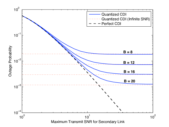
Figure 2: SU outage probability for OCB versus maximum SU-transmit SNR for quantized CDI and perfect IPC feedback

Figs. 2 to Fig. 5 concern OCB with quantized CDI and perfect IPC feedback. Fig. 2 displays the curves of SU outage probability $P_{\mathsf{out}}$ versus maximum SU transmit SNR $\gamma_{\max}$ for the number of cooperative CDI feedback bits $B=\{8,12,16,20\}$. For comparison, we also plot the first-order terms of the $P_{\mathsf{out}}$ limits for large $\gamma_{\max}$ as given in (41). As observed from Fig. 2, with $B$ fixed, $P_{\mathsf{out}}$ converges from above to the corresponding limit as $\gamma_{\max}$ increases, consistent with the result in Corollary 1. The limit of $P_{\mathsf{out}}$ in the interference limiting regime is observed to decrease exponentially with increasing $B$.

Fig. 3 shows that the SU outage probabilities of OCB and NOCB converge as $\gamma_{\max}$ increases, agreeing with Proposition  1. The convergence is slower for larger $B$. However, NOCB significantly outperforms OCB outside the interference limiting regime.

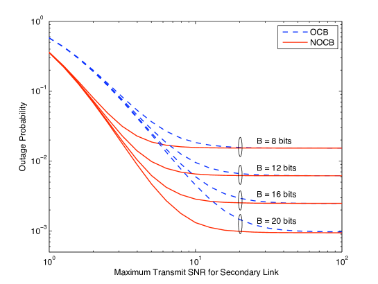
Figure 3: Performance comparison between OCB and NOCB in terms of SU outage probability versus maximum SU transmit SNR. The CDI feedback is quantized and the IPC feedback is assumed perfect.

Fig. 4 illustrates the effects of the SU feedforward on the SU outage probability. The OCB and NOCB beamforming designs are considered in Fig. 4(a) and Fig. 4(b), respectively. It can be observed from both figures that the decrease of the SU outage probability due to feedforward is more significant in the interference limiting regime and for larger $L$. However, increasing $L$ is found to result in higher outage probability in the interference limiting regime, which agrees with the remark on Corollary 1.

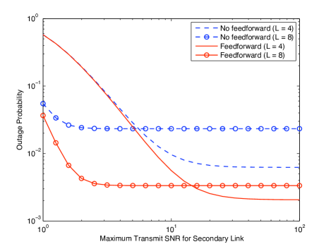
(a) OCB

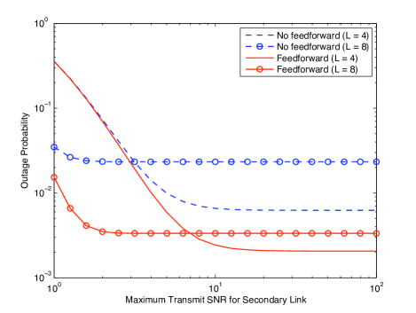
(b) NOCB

Figure 4: SU outage probability versus the maximum SU transmit SNR for (a) OCB and (b) NOCB. For each type of beamforming, both the cases of feedforward and no feedforward are considered. The number of cooperative CDI feedback bits is $B=12$.

Fig. 5 demonstrates the effects of finite-rate ($B^{\prime}$ bits) local feedback and feedforward of ${\mathbf{s}}_{\mathsf{s}}$ on the SU outage probability for OCB with $B=12$ and $B^{\prime}=8$. It can be observed for both OCB and NOCB that the increase of the SU outage probability due to the quantization of ${\mathbf{s}}_{\mathsf{s}}$ is insignificant, justifying the assumption of perfect local feedback and feedforward in the analysis.

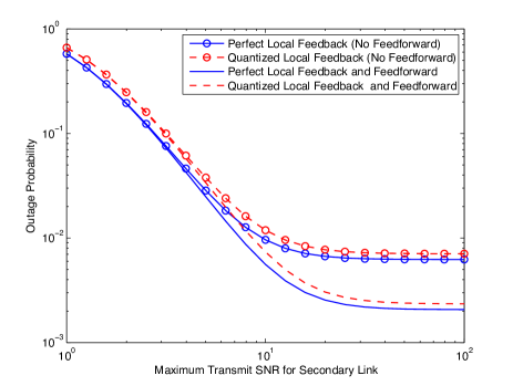
(a) OCB

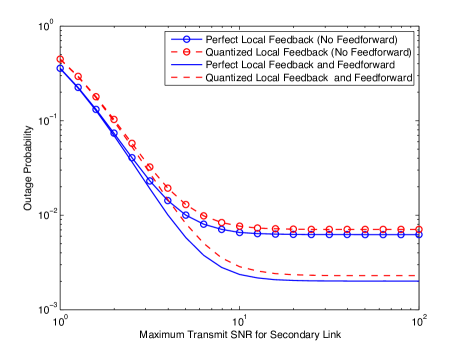
(b) NOCB

Figure 5: Effects of quantizing feedforward and local feedback on the SU outage probability for (a) OCB and (b) NOCB. The number of cooperative CDI feedback bits is $B=12$, and the local feedback/feedforward has $B^{\prime}=8$ bits.

Last, consider both quantized CDI and IPC feedback. Fig. 6 shows the curves of the SU outage probability for the case of OCB without feedforward versus the number of bits $A$ for IPC feedback. It is observed from Fig. 6 that for given $\gamma_{\max}$, there exists an optimal combination of $(A,B)$ that minimizes the outage probability. The optimal values of $A$ are indicated by the marker “o” and those computed using the theoretic result in (57) by the marker “x”. The simulation and theoretic results are closer for larger $\gamma_{\mathsf{p}}$. Specifically, they differ at most by two bits for $\gamma_{\mathsf{p}}=10$ dB (see Fig. 6(a)) and by one bit for $\gamma_{\mathsf{p}}=13$ dB (see Fig. 6(b)). These observations agree with the remark in Section V that the derived feedback tradeoff is a more accurate approximation of the optimal one for larger $\gamma_{\mathsf{p}}$.

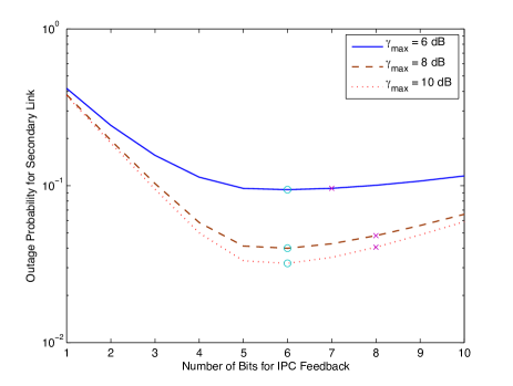
(a) $\gamma_{\mathsf{p}}=10$ dB

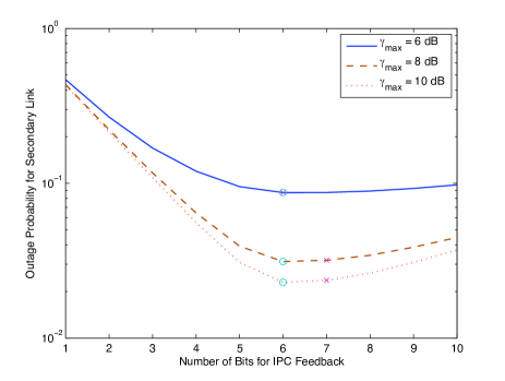
(b) $\gamma_{\mathsf{p}}=13$ dB

Figure 6: SU outage probability versus the number of quantized IPC feedback bits for OCB without feedforward. The PU transmit SNR (a) $\gamma_{\mathsf{p}}=10$ dB and (a) $\gamma_{\mathsf{p}}=13$ dB. The total number of bits for CDI and IPC feedback is $A+B=12$.

VII Concluding Remarks

We have introduced a new operation model for coexisting PU and SU links in a spectrum sharing network, where the PU receiver cooperatively feeds back quantized side information to the SU transmitter for facilitating its opportunistic transmission, such that the resultant PU link performance degradation is minimized. Furthermore, based on cooperative feedback, we have proposed two algorithms for the SU transmit beamforming to improve the SU-link performance. Under a PU-feedback-rate constraint, we have derived the optimal feedback bits allocation for the CDI and IPC feedback. In addition, we have shown that additional cooperative feedforward of the SU CDI from the SU transmitter to the PU receiver further enhances the SU-link performance.

To the authors’ best knowledge, this paper is the first attempt in the literature to study the design of cooperative feedback from the PU to the SU in a cognitive radio network. This work opens several issues worth further investigation. This paper has assumed single antennas for both PU and SU receivers. It is interesting to extend the proposed CB and cooperate feedback schemes to the more general case with MIMO PU and SU links. Moreover, we have assumed a single SU link coexisting with a single PU link, while it is pertinent to investigate the more general system model with multiple coexisting PU and SU links.

-A Proof of Proposition 1

For the case without feedforward, we can expand $\tilde{P}_{\mathsf{out}}$ and $P_{\mathsf{out}}$ as

$$\tilde{P}_{\mathsf{out}} = \Pr(|{\mathbf{f}}_{\mathsf{n}}^{\dagger}{\mathbf{h}}_{\mathsf{s}}|^{2}<\theta_{\mathsf{s}}\sigma^{2})$$ (59)

$$= \left[\Pr(|{\mathbf{f}}_{\mathsf{n}}^{\dagger}{\mathbf{h}}_{\mathsf{s}}|^{2}<\theta_{\mathsf{s}}\sigma^{2}\mid\hat{\mu}_{1}\geq 0,\omega\geq 0)\Pr(\hat{\mu}_{1}\geq 0\mid\omega\geq 0)\right.+$$

$$\left.\Pr(|{\mathbf{f}}_{\mathsf{n}}^{\dagger}{\mathbf{h}}_{\mathsf{s}}|^{2}<\theta_{\mathsf{s}}\sigma^{2}\mid\hat{\mu}_{1}=0,\omega\geq 0)\Pr(\hat{\mu}_{1}=0\mid\omega\geq 0)\right]\Pr(\omega\geq 0)+$$

$$\Pr(|{\mathbf{f}}_{\mathsf{n}}^{\dagger}{\mathbf{h}}_{\mathsf{s}}|^{2}<\theta_{\mathsf{s}}\sigma^{2}\mid\omega<0)\Pr(\omega<0)$$

$$P_{\mathsf{out}} = \Pr(|{\mathbf{f}}_{\mathsf{o}}^{\dagger}{\mathbf{h}}_{\mathsf{s}}|^{2}<\theta_{\mathsf{s}}\sigma^{2})$$ (60)

$$= \Pr(|{\mathbf{f}}_{\mathsf{o}}^{\dagger}{\mathbf{h}}_{\mathsf{s}}|^{2}<\theta_{\mathsf{s}}\sigma^{2}\mid\omega\geq 0)\Pr(\omega\geq 0)+\Pr(|{\mathbf{f}}_{\mathsf{o}}^{\dagger}{\mathbf{h}}_{\mathsf{s}}|^{2}<\theta_{\mathsf{s}}\sigma^{2}\mid\omega<0)\Pr(\omega<0)$$

where $\omega$ is defined in (17) and $\hat{\mu}_{1}$ is the IPC feedback parameter in (32). Using (29) and (32)

$$\lim_{P_{\max}\rightarrow\infty}\Pr(\hat{\mu}_{1}=0\mid\omega\geq 0) = \lim_{P_{\max}\rightarrow\infty}\Pr(\nu<0\mid\omega\geq 0)$$ (61)

$$= 1.$$

Moreover, from Lemma 1 and (32)

$$\lim_{P_{\max}\rightarrow\infty}\Pr(|{\mathbf{f}}_{\mathsf{n}}^{\dagger}{\mathbf{h}}_{\mathsf{s}}|^{2}<\theta_{\mathsf{s}}\sigma^{2}\mid\omega<0) = \lim_{P_{\max}\rightarrow\infty}\Pr\left(P_{\max}<\frac{\theta_{\mathsf{s}}\sigma^{2}}{g_{\mathsf{s}}}\right)$$ (62)

$$= 0.$$

Similarly, it can be shown that

$$\lim_{P_{\max}\rightarrow\infty}\Pr(|{\mathbf{f}}_{\mathsf{o}}^{\dagger}{\mathbf{h}}_{\mathsf{s}}|^{2}<\theta_{\mathsf{s}}\sigma^{2}\mid\omega<0) = 0.$$ (63)

By combining (59), (61), and (62)

$$\lim_{P_{\max}\rightarrow\infty}\tilde{P}_{\mathsf{out}} = \lim_{P_{\max}\rightarrow\infty}\Pr(|{\mathbf{f}}_{\mathsf{n}}^{\dagger}{\mathbf{h}}_{\mathsf{s}}|^{2}<\theta_{\mathsf{s}}\sigma^{2}\mid\hat{\mu}_{1}=0,\omega\geq 0)\Pr(\omega\geq 0)$$ (64)

$$= \lim_{P_{\max}\rightarrow\infty}\Pr(|{\mathbf{f}}_{\mathsf{o}}^{\dagger}{\mathbf{h}}_{\mathsf{s}}|^{2}<\theta_{\mathsf{s}}\sigma^{2}\mid\omega\geq 0)\Pr(\omega\geq 0)$$

where (64) holds since ${\mathbf{f}}_{\mathsf{o}}={\mathbf{f}}_{\mathsf{n}}$ for $\hat{\mu}_{1}=0$. Combining (60), (64) and (63) gives the desired result for the case without feedforward. The proof for the case with feedforward is similar and omitted for brevity.

-B Proof of Lemma 2

Given perfect IPC feedback and the OCB design specified by (9) and (18)

$$\Pr(P_{\mathsf{s}}=P_{\max}) = \bar{P}_{\textsf{out}}+\Pr\left(\frac{\omega}{\lambda g_{\textsf{x}}\epsilon}\geq P_{\max}\right)$$ (65)

where $\bar{P}_{\textsf{out}}$ is given in (4). From the definition of $\omega$ in (17) and define $u=\frac{\theta_{\mathsf{p}}\lambda\gamma_{\max}}{\gamma_{\mathsf{p}}}$, the last term in (65) can be obtained as

$$\Pr\left(\frac{\omega}{\lambda g_{\textsf{x}}\epsilon}\geq P_{\max}\right) = \int\limits_{0}^{2^{-\frac{B}{L-1}}}\int\limits_{0}^{\infty}\int\limits_{\frac{\theta_{\mathsf{p}}}{\gamma_{\mathsf{p}}}(1+\lambda\gamma_{\max}\tau_{2}\tau_{3})}^{\infty}\!f_{g_{\mathsf{p}}}(\tau_{1})f_{g_{\textsf{x}}}(\tau_{2})f_{\epsilon}(\tau_{3})d\tau_{1}d\tau_{2}d\tau_{3}$$

$$= \int\limits_{0}^{2^{-\frac{B}{L-1}}}\int\limits_{0}^{\infty}e^{-\frac{\theta_{\mathsf{p}}}{\gamma_{\mathsf{p}}}(1+\lambda\gamma_{\max}\tau_{2}\tau_{3})}f_{g_{\textsf{x}}}(\tau_{2})f_{\epsilon}(\tau_{3})d\tau_{2}d\tau_{3}$$

$$= \frac{e^{-\frac{\theta_{\mathsf{p}}}{\gamma_{\mathsf{p}}}}}{\Gamma(L)}\int_{0}^{2^{-\frac{B}{L-1}}}\int_{0}^{\infty}\tau_{2}^{L-1}e^{-\left(u\tau_{3}+1\right)\tau_{2}}d\tau_{2}f_{\epsilon}(\tau_{3})d\tau_{3}$$

$$= e^{-\frac{\theta_{\mathsf{p}}}{\gamma_{\mathsf{p}}}}\int_{0}^{2^{-\frac{B}{L-1}}}\frac{f_{\epsilon}(\tau)}{(1+u\tau)^{L}}d\tau$$

$$= e^{-\frac{\theta_{\mathsf{p}}}{\gamma_{\mathsf{p}}}}(L-1)2^{B}\int_{0}^{2^{-\frac{B}{L-1}}}\frac{\tau^{L-2}}{(1+u\tau)^{L}}d\tau$$

$$= e^{-\frac{\theta_{\mathsf{p}}}{\gamma_{\mathsf{p}}}}(L-1)2^{B}\int_{0}^{2^{-\frac{B}{L-1}}}\tau^{L-2}\left[1-Lu\tau+O(\tau^{2})\right]d\tau$$

$$= e^{-\frac{\theta_{\mathsf{p}}}{\gamma_{\mathsf{p}}}}\left[1-(L-1)u2^{-\frac{B}{L-1}}\right]+O\left(2^{-\frac{2B}{L-1}}\right).$$ (67)

The substitution of (67) into (65) gives (36). Next, from (9) and (18),

$$\Pr(P_{\mathsf{s}}<\tau) \!=\! \Pr\left(0\leq\frac{\omega}{\lambda g_{\textsf{x}}\epsilon}\leq\tau\right)$$

$$\!=\! \Pr\left(\omega\geq 0\right)-\Pr\left(\frac{\omega}{\lambda g_{\textsf{x}}\epsilon}\geq\tau\right).$$

Using the above equation, (37) is obtained following similar steps as (67). This completes the proof.

-C Proof of Theorem 1

Since the receive SNR at $\mathsf{R_{\mathsf{s}}}$ is $P_{\mathsf{s}}\tilde{g}_{\mathsf{s}}$,

$$P_{\mathsf{out}} = \Pr(P_{\mathsf{s}}\tilde{g}_{\mathsf{s}}\leq\theta_{\mathsf{s}}\sigma^{2})$$

$$= \int_{0}^{\frac{\theta_{\mathsf{s}}}{\gamma_{\max}}}\Pr(P_{\mathsf{s}}\leq P_{\max})f_{\tilde{g}_{\mathsf{s}}}(\tau)d\tau+\int_{\frac{\theta_{\mathsf{s}}}{\gamma_{\max}}}^{\infty}\Pr\left(P_{\mathsf{s}}\leq\frac{\theta_{\mathsf{s}}\sigma^{2}}{\tau}\right)f_{\tilde{g}_{\mathsf{s}}}(\tau)d\tau$$

$$\overset{(a)}{=} 1-\frac{\Gamma\left(L-1,\frac{\theta_{\mathsf{s}}}{\gamma_{\max}}\right)}{\Gamma(L-1)}+e^{-\frac{\theta_{\mathsf{p}}}{\gamma_{\mathsf{p}}}}\left[\frac{(L-1)\lambda\theta_{\mathsf{p}}\theta_{\mathsf{s}}}{\gamma_{\mathsf{p}}}\right]2^{-\frac{B}{L-1}}\int_{\frac{\theta_{\mathsf{s}}}{\gamma_{\max}}}^{\infty}\frac{\tau^{L-3}}{\Gamma(L-1)}e^{-\tau}d\tau+O\left(2^{-\frac{2B}{L-1}}\right)$$

where (a) uses both Lemmas 2 and 3. The desired result follows from the above equation.

-D Proof of Lemma 4

Define the random variable $\kappa=|{\mathbf{s}}_{1}^{\dagger}{\mathbf{s}}_{2}|^{2}$ where ${\mathbf{s}}_{1}$ and ${\mathbf{s}}_{2}$ are independent isotropic vectors in $\mathds{C}^{L-1}$ with unit norm. The distribution function of $\kappa$ is given as [12]

$$\Pr\left(\kappa>\tau\right)=(1-\tau)^{L-2},\quad 0\leq\tau\leq 1.$$ (68)

As shown in [13], $\delta$ follows the same distribution as $\kappa\epsilon$. Using the above results, the distribution of $\delta$ is readily obtained as follows:

$$\Pr(\delta\leq t) = \Pr(\kappa\epsilon\leq t)$$

$$= \int_{0}^{2^{-\frac{B}{L-1}}}\Pr\left(\kappa\leq\frac{t}{\tau}\right)f_{\epsilon}(\tau)d\tau$$

$$= \int_{0}^{t}\Pr\left(\kappa\leq\frac{t}{\tau}\right)f_{\epsilon}(\tau)d\tau+\int_{t}^{2^{-\frac{B}{L-1}}}\Pr\left(\kappa\leq\frac{t}{\tau}\right)f_{\epsilon}(\tau)d\tau$$

$$= 1-\int_{t}^{2^{-\frac{B}{L-1}}}\Pr\left(\kappa>\frac{t}{\tau}\right)f_{\epsilon}(\tau)d\tau$$

$$\overset{(a)}{=} 1-2^{B}(L-1)\int_{t}^{2^{-\frac{B}{L-1}}}\left(1-\frac{t}{\tau}\right)^{L-2}\tau^{L-2}d\tau$$

$$= 1-2^{B}(L-1)\int_{0}^{2^{-\frac{B}{L-1}}-t}\tau^{L-2}d\tau$$

$$= 1-2^{B}\left(2^{-\frac{B}{L-1}}-t\right)^{L-1}$$ (70)

where (-D) is obtained by substituting (68). Differentiating both sides of (70) gives the desired result.

-E Proof of Lemma 5

Following (65) in the proof of Lemma 2, we can write

$$\Pr(\acute{P}_{\mathsf{s}}=P_{\max})=\bar{P}_{\textsf{out}}+\Pr\left(\frac{\omega}{\lambda g_{\textsf{x}}\delta}\geq P_{\max}\right)$$ (71)

where $\bar{P}_{\textsf{out}}$ is given in (4). Using (-B) with $\epsilon$ replaced by $\delta$, the last term in (71) is obtained as

$$\Pr\left(\frac{\omega}{\lambda g_{\textsf{x}}\delta}\geq P_{\max}\right) = e^{-\frac{\theta_{\mathsf{p}}}{\gamma_{\mathsf{p}}}}\int_{0}^{2^{-\frac{B}{L-1}}}\frac{f_{\delta}(\tau)}{(1+u\tau)^{L}}d\tau$$

$$= e^{-\frac{\theta_{\mathsf{p}}}{\gamma_{\mathsf{p}}}}(L-1)2^{\frac{B}{L-1}}\int_{0}^{2^{-\frac{B}{L-1}}}\left(1-2^{\frac{B}{L-1}}\tau\right)^{L-2}[1-Lu\tau+O(\tau^{2})]d\tau$$

$$= e^{-\frac{\theta_{\mathsf{p}}}{\gamma_{\mathsf{p}}}}\left\{1-(L-1)2^{\frac{B}{L-1}}\int_{0}^{2^{-\frac{B}{L-1}}}\left(1-2^{\frac{B}{L-1}}\tau\right)^{L-2}[Lu\tau+O(\tau^{2})]d\tau\right\}$$

$$= e^{-\frac{\theta_{\mathsf{p}}}{\gamma_{\mathsf{p}}}}\left[1-L(L-1)2^{-\frac{B}{L-1}}b\int_{0}^{1}(1-\tau)^{L-2}\tau d\tau+O\left(2^{-\frac{2B}{L-1}}\right)\right]$$ (73)

$$= e^{-\frac{\theta_{\mathsf{p}}}{\gamma_{\mathsf{p}}}}\left[1-L(L-1)2^{-\frac{B}{L-1}}b\mathcal{B}(2,L-1)+O\left(2^{-\frac{2B}{L-1}}\right)\right]$$

where (-E) applies Lemma 4 and $\mathcal{B}(\cdot,\cdot)$ represents the beta function. By substituting $\mathcal{B}(x,y)=\frac{\Gamma(x)\Gamma(y)}{\Gamma(x+y)}$ [23, 8.384] into (73)

$$\Pr\left(\frac{\omega}{\lambda g_{\textsf{x}}\delta}\geq P_{\max}\right) = e^{-\frac{\theta_{\mathsf{p}}}{\gamma_{\mathsf{p}}}}\left[1-L(L-1)2^{-\frac{B}{L-1}}b\frac{\Gamma(2)\Gamma(L-1)}{\Gamma(L+1)}+O\left(2^{-\frac{2B}{L-1}}\right)\right]$$ (74)

$$= e^{-\frac{\theta_{\mathsf{p}}}{\gamma_{\mathsf{p}}}}\left[1-2^{-\frac{B}{L-1}}b+O\left(2^{-\frac{2B}{L-1}}\right)\right]$$

where (74) uses $\Gamma(L+1)=L!$. Substituting (4) and (74) into (71) gives (45). The desired result in (46) can be obtained following similar steps as given above.

-F Proof of Lemma 6

Based on the IPC feedback quantization algorithm in Section III-A2 and for $1\leq n\leq n_{0}$

$$\Pr(p_{n-1}\leq\eta\leq p_{\mathsf{n}}\mid\gamma_{\mathsf{p}}g_{\mathsf{p}}\geq\theta_{\mathsf{p}}) = \frac{\Pr(p_{n-1}\leq P_{\mathsf{s}}<p_{\mathsf{n}})}{\Pr(\gamma_{\mathsf{p}}g_{\mathsf{p}}\geq\theta_{\mathsf{p}})}$$ (75)

$$= \frac{(L-1)\theta_{\mathsf{p}}\lambda 2^{-\frac{B}{L-1}}}{\gamma_{\mathsf{p}}\sigma^{2}}(p_{\mathsf{n}}-p_{n-1})+O\left(2^{-\frac{2B}{L-1}}\right)$$

where (75) uses Lemma 2. Combining (20), (75) and $N=2^{A}$ gives

$$p_{n}-p_{n-1}=\frac{\gamma_{\mathsf{p}}\sigma^{2}}{(L-1)\theta_{\mathsf{p}}\lambda}2^{\frac{B}{L-1}-A}+O\left(2^{-\frac{B}{L-1}}\right),\quad 1\leq n\leq n_{0}.$$ (76)

The desired result follows from (48) and (76).

-G Proof of Lemma 7

The equality in (50) follows from the quantized IPC feedback algorithm in Section III-A2. Based on this algorithm

$$\Pr(\hat{P}_{\mathsf{s}}<\tau)\!\!\! = \!\!\!\Pr\left(0\leq\left\lfloor\frac{\omega}{\lambda g_{\textsf{x}}\epsilon}\right\rfloor_{\mathcal{P}}\leq\tau\right)$$ (77)

$$\leq \Pr\left(0\leq\frac{\omega}{\lambda g_{\textsf{x}}\epsilon}\leq\tau+\Delta P\right)$$

$$\leq \Pr\left(\omega\geq 0\right)-\Pr\left(\frac{\omega}{\lambda g_{\textsf{x}}\epsilon}\geq(\tau+\Delta P)\right)$$ (78)

where (77) follows from (48). The desired result in (51) is obtained using (78) and following similar steps as deriving $\Pr(P_{\mathsf{s}}<\tau)$ in Lemma 2.

References

- [1] A. Goldsmith, S. Jafar, I. Maric, and S. Srinivasa, “Breaking spectrum gridlock with cognitive radios: An information theoretic perspective,” Proceedings of the IEEE, vol. 97, pp. 894–914, May 2009.
- [2] R. Zhang and Y. C. Liang, “Exploiting multi-antennas for opportunistic spectrum sharing in cognitive radio networks,” IEEE Journal on Sel. Topics in Signal Processing, vol. 2, pp. 88–102, Feb. 2008.
- [3] R. Zhang, F. Gao, and Y. C. Liang, “Cognitive beamforming made practical: Effective interference channel and learning-throughput tradeoff,” IEEE Trans. on Communications, vol. 58, pp. 706–718, Feb. 2010.
- [4] L. Zhang, Y.-C. Liang, Y. Xin, and H. V. Poor, “Robust cognitive beamforming with partial channel state information,” IEEE Trans. on Communications, vol. 8, pp. 4143–453, Aug. 2009.
- [5] Y. Chen, G. Yu, Z. Zhang, H. Chen, and P. Qiu, “On cognitive radio networks with opportunistic power control strategies in fading channels,” IEEE Trans. on Wireless Communications, vol. 7, pp. 2752–2761, Jul. 2008.
- [6] R. Zhang, “Optimal power control over fading cognitive radio channels by exploiting primary user CSI,” in Proc., IEEE Globecom, Nov. 2008.
- [7] A. Scaglione, P. Stoica, S. Barbarossa, G. B. Giannakis, and H. Sampath, “Optimal designs for space-time linear precoders and decoders,” IEEE Trans. on Sig. Proc., vol. 50, pp. 1051–1064, May 2002.
- [8] D. J. Love, R. W. Heath Jr., W. Santipach, and M. L. Honig, “What is the value of limited feedback for MIMO channels?,” IEEE Communications Magazine, vol. 42, pp. 54–59, Oct. 2004.
- [9] D. J. Love, R. W. Heath, V. K. N. Lau, D. Gesbert, B. D. Rao, and M. Andrews, “An overview of limited feedback in wireless communication systems,” IEEE Journal on Sel. Areas in Communications, vol. 26, no. 8, pp. 1341–1365, 2008.
- [10] D. J. Love, R. W. Heath Jr., and T. Strohmer, “Grassmannian beamforming for MIMO wireless systems,” IEEE Trans. on Inform. Theory, vol. 49, pp. 2735–2747, Oct. 2003.
- [11] V. K. N. Lau, Y. Liu, and T.-A. Chen, “On the design of MIMO block-fading channels with feedback-link capacity constraint,” IEEE Trans. on Communications, vol. 52, pp. 62–70, Jan. 2004.
- [12] K. K. Mukkavilli, A. Sabharwal, E. Erkip, and B. Aazhang, “On beamforming with finite rate feedback in multiple antenna systems,” IEEE Trans. on Inform. Theory, vol. 49, pp. 2562–79, Oct. 2003.
- [13] N. Jindal, “MIMO broadcast channels with finite-rate feedback,” IEEE Trans. on Inform. Theory, vol. 52, pp. 5045–5060, Nov. 2006.
- [14] M. Sharif and B. Hassibi, “On the capacity of MIMO broadcast channels with partial side information,” IEEE Trans. on Inform. Theory, vol. 51, pp. 506–522, Feb. 2005.
- [15] K.-B. Huang, R. W. Heath Jr., and J. G. Andrews, “SDMA with a sum feedback rate constraint,” IEEE Trans. on Sig. Proc., vol. 55, pp. 3879–91, July 2007.
- [16] Q. Zhao and B. M. Sadler, “A survey of dynamic spectrum access,” IEEE Signal Processing Magazine, vol. 24, pp. 79–89, May 2007.
- [17] Third Generation Partnership Project: LTE-Advanced. Online: http://www.3gpp.org/article/lte-advanced.
- [18] T. Yoo, N. Jindal, and A. Goldsmith, “Multi-antenna broadcast channels with limited feedback and user selection,” IEEE Journal on Sel. Areas in Communications, vol. 25, pp. 1478–1491, July 2007.
- [19] S. Zhou, Z. Wang, and G. B. Giannakis, “Quantifying the power loss when transmit beamforming relies on finite-rate feedback,” IEEE Trans. on Communications, vol. 4, pp. 1948–1957, July 2005.
- [20] T. K. Y. Lo, “Maximum ratio transmission,” IEEE Trans. on Communications, vol. 47, pp. 1458–1461, Oct. 1999.
- [21] S. P. Lloyd, “Least square quantization in PCM’s,” Bell Telephone Lab. Paper, 1957.
- [22] N. Jindal, J. G. Andrews, and S. Weber, “Multi-antenna communication in ad hoc networks: achieving MIMO gains with SIMO transmission,” submitted to IEEE Trans. on Communications.
- [23] I. Gradshteyn and I. Ryzhik, Table of integrals, series, and products. Academic Press, 7 ed., 2007.