Towards an ‘average’ version of the Birch and Swinnerton-Dyer Conjecture

Abstract.

The Birch and Swinnerton-Dyer conjecture states that the rank of the Mordell-Weil group of an elliptic curve $E$ equals the order of vanishing at the central point of the associated L-function $L(s,E)$. Previous investigations have focused on bounding how far we must go above the central point to be assured of finding a zero, bounding the rank of a fixed curve or on bounding the average rank in a family. Mestre [Mes] showed the first zero occurs by $O(1/\log\log N_{E})$, where $N_{E}$ is the conductor of $E$, though we expect the correct scale to study the zeros near the central point is the significantly smaller $1/\log N_{E}$. We significantly improve on Mestre’s result by averaging over a one-parameter family of elliptic curves, obtaining non-trivial upper and lower bounds for the average number of normalized zeros in intervals on the order of $1/\log N_{E}$ (which is the expected scale). Our results may be interpreted as providing further evidence in support of the Birch and Swinnerton-Dyer conjecture, as well as the Katz-Sarnak density conjecture from random matrix theory (as the number of zeros predicted by random matrix theory lies between our upper and lower bounds). These methods may be applied to additional families of $L$-functions.

1. Introduction

The goal of this paper is to provide evidence towards the Birch and Swinnerton-Dyer conjecture in one-parameter families of elliptic curves. We briefly summarize our results, assuming the reader is familiar with the notation and subject. Afterwards we review the needed background material from elliptic curves and previous results in §2; for the convenience of the reader, we state all the conjectures assumed or discussed at various points in Appendix A. We then prove our theorems and discuss generalizations to other families of $L$-functions in §3, where we give explicit non-trivial upper and lower bounds.

The Birch and Swinnerton Dyer conjecture asserts that if $E$ is an elliptic curve whose Mordell-Weil group $E(\mathbb{Q})$ has geometric rank $r$, then the associated completed $L$-function $\Lambda(s,E)$ has analytic rank $r$ (i.e., it vanishes to order $r$ at the central point). This is an exceptionally hard problem to investigate, theoretically and numerically. While there is some theoretical evidence when the rank is at most 1, the general case is intractable both theoretically and experimentally. For example, although we can construct elliptic curves with geometric rank exceeding 20, the largest known lower bound for the analytic rank of a $\Lambda(s,E)$ is only 3.

We consider the following natural question. Let $E$ be an elliptic curve with geometric rank $r$, and assume the Generalized Riemann Hypothesis (GRH). The Birch and Swinnerton-Dyer conjecture predicts that there should be $r$ zeros at the central point. How far must we go along the critical line before we are assured of seeing $r$ zeros?

If $N_{E}$ denotes the conductor of the elliptic curve, we expect the correct scale for zeros near the central point to be of size $1/\log N_{E}$. Miller [Mil3] investigated the first few zeros above the central point for the family of all elliptic curves as well as one-parameter families of small rank over $\mathbb{Q}(T)$. His results are consistent with the low zeros being of height on the order of $1/\log N_{E}$; however, the first few zeros are higher than the $N_{E}\to\infty$ scaling limits predicted by the independent model of random matrix theory. The data suggests that, for finite conductors, better agreement is obtained by modeling these zeros with the interaction model (which involves Jacobi ensembles). Determining the correct corresponding random matrix ensemble involves understanding the discretization of the central values of $L$-functions and the lower order terms in the 1-level density. In his thesis Duc Khiem Huyn [Huy] successfully modeled the first zero of the family of quadratic twists of a fixed elliptic curve, and current work by the second named author and Eduardo Dueñez, Duc Khiem Huynh, Jon Keating and Nina Snaith is investigating the case of a general one-parameter family [DHKMS].

The best theoretical result on the first zero above the central point is due to Mestre. Assuming the Generalized Riemann Hypothesis, Mestre [Mes] bounded the analytic rank of $E$ by $O(\log N_{E}/\log\log N_{E})$ and showed its first zero above the central point is at most $B/\log\log N_{E}$. While this is significantly larger than what we expect the truth to be, namely $O(1/\log N_{E})$, it has the advantage of holding for all elliptic curves.

In this note we show that we may reduce the window on the critical line to something of the expected order if we average over a one-parameter family of elliptic curves. Specifically, consider a one-parameter family $\mathcal{E}:y^{2}=x^{3}+A(T)x+B(T)$ of geometric rank $r$ over $\mathbb{Q}(T)$, with $A(T),B(T)\in\mathbb{Z}[T]$. For each $t\in\mathbb{Z}$ we may specialize and obtain an elliptic curve $E_{t}:y^{2}=x^{3}+A(t)x+B(t)$ with conductor $N_{t}:=N_{E_{t}}$. By Silverman’s specialization theorem [Sil2], for all $t$ sufficiently large each elliptic curve $E_{t}$ has geometric rank at least $r$. Assuming standard conjectures, Helfgott [He] proved that for a generic family the sign of the functional equation is 1 half the time and -1 the other half. It is believed that a generic curve in a generic family has analytic rank as small as possible consistent with all constraints. In our case, as the rank must be at least $r$ if the Birch and Swinnerton-Dyer conjecture is true, we expect that in the limit half the curves will have analytic rank $r$ and the other half $r+1$, for an average rank of $r+\frac{1}{2}$.

We take our family to be $\mathcal{F}_{R}:=\{\Lambda(s,E_{t}):R\leq t\leq 2R\}$ with $R\to\infty$, though we often abuse notation and use $\mathcal{F}_{R}$ to denote $t$ in $[R,2R]$. There are two ways to normalize the zeros of $\Lambda(s,E_{t})$ near the central point: (1) globally, using $\frac{\log N}{2\pi}:=\frac{1}{R}\sum_{t\in\mathcal{F}_{R}}\frac{\log N_{t}}{2\pi}$; (2) locally, using $\frac{\log N_{t}}{2\pi}$. It is significantly easier to use the global rescaling; however, as each elliptic curve can be considered independent of the family, it is more correct to use the local rescaling (in this case, due to the technicalities that arise we must add some additional restrictions on which $t\in[R,2R]$ are in the family).

Before stating our main result, we must first introduce some notation. All conjectures are stated in full in Appendix A.

Definition 1.1 (Sieved family).

Let $\mathcal{E}:y^{2}=x^{3}+A(T)x+B(T)$ be a one-parameter family of elliptic curves over $\mathbb{Q}(T)$ with discriminant $\Delta(T)$, let $D(T)$ be the product of the irreducible polynomial factors of the discriminant, and let $B$ be the largest square dividing $D(t)$ for all integers $t$. For a fixed $c,t_{0}$, our family is the set of all $t=ct^{\prime}+t_{0}$ (with $t\in[R,2R]$) such that $D(ct^{\prime}+t_{0})$ is square-free except for primes $p|B$ where the power of such $p|D(t)$ is independent of $t$. In [Mil2] it is shown that for any one-parameter family, there is a choice of $c$ and $t_{0}$ such that the number of such $t$ is $c_{\mathcal{E}}R+o(R)$ for some $c_{\mathcal{E}}>0$ if every irreducible polynomial factor of $\Delta(T)$ has degree at most 3 (if not, the claim is true if we assume either the ABC or Square-free Sieve Conjecture). We let $\mathcal{F}_{R}^{\prime}$ denote the sieved family.

Definition 1.2 (Average number of zeros in a family).

Let $\mathcal{E}:y^{2}=x^{3}+A(T)x+B(T)$ be a one-parameter family of elliptic curves over $\mathbb{Q}(T)$ with specialized curves $E_{t}$ with conductors $N_{t}$. Assume GRH and write the non-trivial zeros of $\Lambda(s,E_{t})$ as $\frac{1}{2}+i\gamma_{t,j}$, and set

$$\frac{\log N}{2\pi}\ :=\ \frac{1}{R}\sum_{t=R}^{2R}\frac{\log N_{t}}{2\pi}.$$ (1.1)

The average number of zeros with imaginary part at most $\tau$ (in absolute value) under the global and local renormalizations are defined to be

$$Z_{{\rm ave},\mathcal{E},R}^{({\rm global})}(\tau) \ :=\ \frac{1}{R}\sum_{t=R}^{2R}\#\left\{j:\gamma_{t,j}\frac{\log N}{2\pi}\in[-\tau,\tau]\right\}$$

$$Z_{{\rm ave},\mathcal{E},R}^{({\rm local})}(\tau) \ :=\ \frac{1}{|\mathcal{F}_{R}\ ^{\prime}|}\sum_{t=R\atop t\in\mathcal{F}_{R}^{\prime}}^{2R}\#\left\{j:\gamma_{t,j}\frac{\log N_{t}}{2\pi}\in[-\tau,\tau]\right\}.$$ (1.2)

The Birch and Swinnerton-Dyer conjecture implies that, for families where half the curves have even and half have odd sign,

$$Z_{{\rm ave},\mathcal{E},R}^{({\rm global})}(0)\ =\ Z_{{\rm ave},\mathcal{E},R}^{({\rm local})}(0)\ \geq\ r+\frac{1}{2}.$$

Our main results are upper and lower bounds for how many normalized zeros there are on average in the interval $[-\tau,\tau]$, in particular, how small we may take $\tau$ and be assured on average that there are $r+\frac{1}{2}$ zeros in the interval.

Theorem 1.3.

Let $\mathcal{E}$ be a one-parameter family of elliptic curves of geometric rank $r$ over $\mathbb{Q}(T)$; if $\mathcal{E}$ is not a rational surface (see Remark A.1 for a definition) then assume Tate’s conjecture. Additionally, if we are using the local renormalization of the zeros we must assume either the ABC or the Square-free Sieve Conjecture if the discriminant has an irreducible polynomial factor of degree at least 4.

Let $\sigma$ be chosen such that we can compute the $1$-level density (defined in §2.3) for even Schwartz test functions $\phi$ with ${\rm supp}(\mathaccent 866{\phi})\subset(-\sigma,\sigma)$; see Theorem 2.3 for details on what $\sigma$ are permissible for a given family.

Then

• Lower bounds for the average number of normalized zeros in $[-\tau,\tau]$: Let the notation be as in Definition 1.2, and assume GRH. Let $h$ be any even, twice continuously differentiable function supported on $[-1,1]$ and monotonically decreasing on $[0,1]$. For fixed $\tau>0$ let $f(y)=h(2y/\sigma)$, $g(y)=(f\ast f)(y)$ (the convolution of $f$ with itself), and let $\phi(x)$ equal the Fourier transform of $g(y)+(2\pi\tau)^{-2}g^{\prime\prime}(y)$. Note ${\rm supp}(\mathaccent 866{\phi})\subset(-\sigma,\sigma)$ and $\phi(x)$ is non-negative for $|x|<\tau$ and non-positive for $|x|>\tau$. Then

  $$Z_{{\rm avg},\mathcal{E},R}^{({\rm global})}(\tau),\ Z_{{\rm avg},\mathcal{E},R}^{({\rm local})}(\tau)\ \ \geq\ \left(r+\frac{1}{2}\right)+\frac{\mathaccent 866{\phi}(0)}{\phi(0)}+O\left(\frac{\log\log R}{\phi(0)\log R}\right),$$ (1.3)

  where

  $$\frac{\mathaccent 866{\phi}(0)}{\phi(0)}\ =\ \frac{(\int_{0}^{1}h(u)^{2}du)+(\frac{1}{\sigma\tau\pi})^{2}(\int_{0}^{1}h(u)h^{\prime\prime}(u)du)}{\sigma(\int_{0}^{1}h(u)du)^{2}}.$$ (1.4)

  If we let $\tau_{\rm BSD}(\sigma)$ denote the value of $\tau$ such that we are assured of at least $r+\frac{1}{2}$ zeros on average (as $R\to\infty$) in $[-\tau,\tau]$ given that we can compute the 1-level density for test functions whose Fourier transform is supported in $(-\sigma,\sigma)$, then

  $$\tau_{\rm BSD}(\sigma)\ \leq\ \frac{1}{\pi}\left(-\frac{\int_{0}^{1}h(u)^{2}du}{\int_{0}^{1}h(u)h^{\prime\prime}(u)du}\right)^{-1/2}\ \frac{1}{\sigma}\ :=\ \frac{1}{\pi C(h)\sigma}.$$ (1.5)

  This should be compared to the predictions from the Birch and Swinnerton-Dyer and Parity Conjectures for a generic family, which predict $\tau_{{\rm BSD}}(\sigma)=0$. In particular, taking

  $$h(x)\ =\ \begin{cases}(1-x^{2})(1-0.233428x^{2}+0.0189588x^{4})&\text{if $|x|\leq 1$}\\ 0&\text{otherwise}\end{cases}$$ (1.6)

  yields

  $$\tau_{{\rm BSD}}(\sigma)\ \leq\ \frac{1}{\pi C(h)\sigma},$$ (1.7)

  where $C(h)\approx 0.63662$ (which is approximately $2/\pi$); note $1/\pi C(h)\sigma$ is approximately $1/2\sigma$. In the arguments below we use $2/\pi$ for brevity without reminding the reader that the numerical calculation is only close to the above.
  

• Upper bounds for the average number of normalized zeros in $[-\tau,\tau]$: Let $\psi$ be a twice continuously differentiable even Schwartz test function with ${\rm supp}(\mathaccent 866{\psi})\subset(-\sigma,\sigma)$, $\psi(x)\geq 0$ for all $x$, and $\psi(x)$ monotonically decreasing on $\left[0,\tau\right)$. Then

  $$Z_{{\rm ave},\mathcal{F},R}^{({\rm global})}(\tau),\ Z_{{\rm ave},\mathcal{F},R}^{({\rm local})}(\tau)$$

  $$\ \ \ \ \ \ \ \ \ \leq\ \left(r+\frac{1}{2}\right)+\frac{(r+\frac{1}{2})(\psi(0)-\psi(\tau))+\hat{\psi}(0)}{\psi(\tau)}+O\left(\frac{\log\log R}{\psi(0)\log R}\right).$$ (1.8)

  If we consider the interval $(-\frac{1}{2\sigma},\frac{1}{2\sigma})$ from the lower bound, taking $\psi(x)=\left(\frac{\sin{x\pi\sigma}}{x\pi\sigma}\right)^{2}$ yields the average number of normalized zeros in the limit in this interval is at most $\Big{(}r+\frac{1}{2}$ $+$ $\frac{1}{\sigma}\Big{)}/\psi(1/2\sigma)=\frac{\pi^{2}}{4}$ $\Big{(}r+\frac{1}{2}$ $+$ $\frac{1}{\sigma}\Big{)}$.

• Random matrix theory prediction. Let $\mathcal{E}$ be a generic one-parameter family of elliptic curves of rank $r$ over $\mathbb{Q}(T)$ with half of the specialized functional equations even and half odd. Assuming the Katz-Sarnak Density Conjecture, as $R\to\infty$ the average number of normalized zeros in $[-\tau,\tau]$ is $(r+\frac{1}{2})+2\tau$; more precisely, random matrix theory predicts

  $$\lim_{R\to\infty}Z_{{\rm ave},\mathcal{F},R}^{({\rm global})}(\tau),\ Z_{{\rm ave},\mathcal{F},R}^{({\rm local})}(\tau)\ =\ r+\frac{1}{2}+2\tau.$$ (1.9)

  In particular, setting $\tau=\frac{1}{2\sigma}$ yields a prediction of $r+\frac{1}{2}+2\cdot\frac{1}{2\sigma}$ normalized zeros in the limit on average.

In summary, the number of normalized zeros on average as $R\to\infty$ in the interval $\left(-\frac{1}{2\sigma},\frac{1}{2\sigma}\right)$ satisfy

$$r+\frac{1}{2}\ \leq\ Z_{{\rm ave},\mathcal{E},R}^{({\rm global})}(\tau),\ Z_{{\rm ave},\mathcal{E},R}^{({\rm local})}(\tau)\ \leq\ \frac{\pi^{2}}{4}\left(r+\frac{1}{2}+\frac{1}{\sigma}\right),$$ (1.10)

and this interval contains the prediction from Random Matrix Theory, $r+\frac{1}{2}+\frac{1}{\sigma}$.

Remark 1.4.

We obtained our upper bound for $\tau_{\rm BSD}(\sigma)$ by setting $\mathaccent 866{\phi}(0)/\phi(0)=0$. The important item to note is that $\tau_{\rm BSD}(\sigma)$ (or any $\tau$) is inversely proportional to the support $\sigma$. In other words, the larger we may take $\sigma$, the more we may concentrate $\phi$ near the central point and thus the smaller the window. Random matrix theory predicts we may take $\sigma$ arbitrarily large, which would imply we may take $\tau$ arbitrarily small and thus prove the Birch and Swinnerton-Dyer conjecture on average.

2. Background material and previous results

2.1. Elliptic curves

We quickly review the needed background material on elliptic curves; the reader familiar with the notation and theory may safely skip this subsection. See [Kn, Kob, Sil1, ST] for proofs, as well as the survey [Yo1].

Let $E$ be an elliptic curve over $\mathbb{Q}$, say $y^{2}=x^{3}+ax+b$ with $a,b\in\mathbb{Z}$, and set

$$E(\mathbb{Q})\ :=\ \{(x,y)\in\mathbb{Q}^{2}:y^{2}=x^{3}+ax+b\}.$$ (2.1)

We can define addition of two elements of $E(\mathbb{Q})$ as follows (see Figure 1).

Figure 1. The addition law on an elliptic curve. In the second example the line is tangent to $E$ at $P$.

If $P=(x_{1},y_{1})$ and $Q=(x_{2},y_{2})$ are in $E(\mathbb{Q})$, then the line $y=mx+b$ connecting them has rational coordinates. Substituting this expression for $y$ into the elliptic curve, we find $(mx+b)^{2}=x^{3}+ax+b$. This is a cubic in $x$ with rational coefficients. By construction two of its roots are $x_{1}$ and $x_{2}$, both rational numbers. Thus the third root, say $x_{3}$, must also be rational. Set $R(P,Q)=(x_{3},\sqrt{x_{3}^{3}+ax_{3}+b})$ and $\mathaccent 869{R}(P,Q)=(x_{3},-\sqrt{x_{3}^{3}+ax_{3}+b})$. If we define addition by $P\oplus Q=\mathaccent 869{R}(P,Q)$, then this (plus adding a ‘point at infinity’) turns $E(\mathbb{Q})$ into a finitely generated abelian group. We write $E(\mathbb{Q})$ as $\mathbb{Z}^{r}\oplus\mathbb{T}$, where $\mathbb{T}$ is a torsion group and $r$ is called the geometric rank of the curve.

Given an elliptic curve $E$ as above, we may associate an $L$-function as follows. Assume $y^{2}=x^{3}+ax+b$ is a globally minimal Weierstrass equation for $E/\mathbb{Q}$ with discriminant $\Delta=-16(4a^{3}+27b^{2})$ and conductor $N_{E}$. Set

$$a_{E}(p)\ :=\ p-\#\{(x,y)\in(\mathbb{Z}/p\mathbb{Z})^{2}:y^{2}\equiv x^{3}+ax+b\bmod p\}.$$ (2.2)

Note that the $a_{E}(p)$’s encode local data, specifically the number of solutions modulo $p$. Hasse proved $|a_{E}(p)|\leq 2\sqrt{p}$, and we define the $L$-function by

$$L(s,E)\ :=\ \prod_{p|\Delta}\left(1-\frac{a_{E}(p)}{\sqrt{p}}p^{-s}\right)^{-1}\prod_{p\mathchar 13613\relax\Delta}\left(1-\frac{a_{E}(p)}{\sqrt{p}}p^{-s}+p^{-2s}\right)^{-1};$$ (2.3)

we have included the factors of $\sqrt{p}$ so that the completed $L$-function has a functional equation from $s$ to $1-s$ and not $2-s$:

$$\Lambda(s,E)\ :=\ \left(\frac{\sqrt{N}}{2\pi}\right)^{s}\Gamma\left(s+\frac{1}{2}\right)L(s,E)\ =\ \epsilon_{E}\Lambda(1-s,E),$$ (2.4)

where $\epsilon_{E}\in\{1,-1\}$ is the sign of the functional equation. Following the work of Wiles [Wi], Taylor-Wiles [TW] and Breuil-Conrad-Diamond-Taylor [BCDT], we may associate a weight 2 modular form $f$ to any elliptic curve $E$, where the level of $f$ equals the conductor $N_{E}$ of $E$. We have $\Lambda(s,f)=\Lambda(s,E)$; in particular, the completed $L$-function converges for all $s$. We call the order of vanishing of $\Lambda(s,E)$ at $s=1/2$ the analytic rank of $E$.

The Birch and Swinnerton-Dyer conjecture [BS-D1, BS-D2] states that the order of vanishing of $\Lambda(s,E)$ at the central point $s=1/2$ equals the rank of the Mordell-Weil group $E(\mathbb{Q})$, or that the analytic rank equals the geometric rank. Sadly, we are far from being able to prove this, though the evidence for the conjecture is compelling, especially in the case of complex multiplication and rank at most 1 [Bro, CW, GKZ, GZ, Kol1, Kol2, Ru]. In addition there is much suggestive numerical evidence for the conjecture; for example, for elliptic curves with modest geometric rank $r$, numerical approximations of the first $r-1$ Taylor coefficients are consistent with these coefficients vanishing.

2.2. Explicit Formula

One powerful tool for investigating the Birch and Swinnerton-Dyer conjecture is the Explicit Formula (see [RS] for a proof for a general $L$-function, or [Mil1] for the calculation for elliptic curves), which connects the zeros of an $L$-functions to the Fourier coefficients.

Theorem 2.1.

Let $\phi$ be an even, twice continuously differentiable test-function whose Fourier transform

$$\mathaccent 866{\phi}(y)\ :=\ \int_{-\infty}^{\infty}\phi(x)e^{-2\pi ixy}dx$$ (2.5)

has compact support, and denote the non-trivial zeros of $\Lambda(s,E)$ by $\frac{1}{2}+i\gamma_{E}^{(j)}$ (under the Generalized Riemann Hypothesis, each $\gamma_{E}^{(j)}\in\mathbb{R}$). Then

$$\sum_{\gamma_{E}^{(j)}}\phi\left(\gamma_{E}^{(j)}\frac{\log N_{E}}{2\pi}\right) = \mathaccent 866{\phi}(0)+\phi(0)-2\sum_{p}\frac{a_{E}(p)\log p}{p\log N_{E}}\ \mathaccent 866{\phi}\left(\frac{\log p}{\log N_{E}}\right)$$ (2.6)

$$-2\sum_{p}\frac{a_{E}^{2}(p)\log p}{p^{2}\log N_{E}}\ \mathaccent 866{\phi}\left(\frac{2\log p}{\log N_{E}}\right)+O\left(\frac{\log\log N_{E}}{\log N_{E}}\right).\ \ \ \ \ \ \ \ \ \$$

Using the explicit formula, Mestre proved

Theorem 2.2 (Mestre [Mes]).

Assuming the Generalized Riemann Hypothesis:

1. The order of vanishing at the central point is $O(\log N_{E}/\log\log N_{E})$.

2. There is an absolute constant $B$ such that the first zero above the central point occurs before $B/\log\log N_{E}$.

From the functional equation, however, we expect the first zero above the central point to be on the order of $1/\log N_{E}$, and not $1/\log\log N_{E}$. Thus Mestre’s result is significantly larger than what we expect the truth to be; however, it holds for any elliptic curve. The situation is very different if instead we consider families of elliptic curves. By averaging the explicit formula over the family and exploiting cancelation in the sums of the Fourier coefficients $a_{E}(p)$, it is possible to prove (on average) significantly better results.

Numerous studies have been concerned with bounding the average rank in families. We list some of the frequently studied families below (note that, for technical reasons, often one has to do some sieving and remove some curves in order to make certain sums tractable). These results are obtained by averaging the explicit formula over some family $\mathcal{F}_{R}$, where $R$ is a parameter localizing the conductors, and sending $R\to\infty$.

• The family of all elliptic curves: $y^{2}=x^{3}+Ax+B$, and $\mathcal{F}_{R}=\{(A,B):|A|\leq R^{2},|B|\leq R^{3}\}$ (or something along these lines).

• One parameter families over $\mathbb{Q}(T)$: $y^{2}=x^{3}+A(T)x+B(T)$, with $A(T)$, $B(T)$ $\in$ $\mathbb{Z}[T]$ and either $\mathcal{F}_{R}=\{t:R\leq t\leq 2R\}$ or a sub-family of this where the conductors are given by a polynomial.

• Quadratic (or higher) twists of a fixed elliptic curve: $dy^{2}=x^{3}+ax+b$, with $\mathcal{F}_{R}=\{d:d\leq R\ {\rm a\ fundamental\ discriminant}\}$.

The current record belongs to M. Young [Yo2], who showed the average rank in the family of all elliptic curves is bounded by $25/14\approx 1.79$; results for one-parameter families and quadratic twist families are significantly worse. For a sample of the literature, see [BMSW, Bru, BM, CPRW, DFK, Gao, Go, GM, H-B, Kow1, Kow2, Mi, Mil2, RSi, RuSi, Sil3, Yo2, ZK] (especially the surveys [BMSW, Kow1, RuSi]).

2.3. The one-level density

For a family $\mathcal{F}_{R}$ of $L$-functions ordered by conductor (with $R\to\infty$), the averaged explicit formula is called the one-level density. Specifically, let $\phi$ be an even Schwartz test-function whose Fourier transform is supported in $(-\sigma,\sigma)$, and denote the zeros of $L(s,f)$ by $1/2+i\gamma_{f,\ell}$ (under GRH each $\gamma_{f,\ell}\in\mathbb{R}$). Let $N_{f}$ denote the analytic conductor of $L(s,f)$. We define the one-level density by

$$D_{\mathcal{F}_{R}}(\phi)\ :=\ \frac{1}{|\mathcal{F}_{R}|}\sum_{f\in\mathcal{F}_{R}}\sum_{f}\phi\left(\gamma_{f}^{(j)}\frac{\log N_{f}}{2\pi}\right).$$ (2.7)

This statistic has been fruitfully used by many researchers to study the zeros of elliptic curves $L$-functions (as well as other families of $L$-functions) near the central point.

Unlike the $n$-level correlations, which are the same for any cuspidal newform arising from an automorphic representation (see [Hej, Mon, RS]), the one-level density for a family of $L$-functions depends on the symmetry of the family. Katz and Sarnak [KS1, KS2] conjecture that families of $L$-functions correspond to classical compact groups; specifically, the behavior as the conductors tend to infinity of zeros (respectively values) of $L$-functions is well-modeled by the limit as the matrix size tends to infinity of roots (respectively values) of characteristic values of random matrices. They conjecture that

$$\lim_{R\to\infty}D_{\mathcal{F}_{R}}(\phi)\ =\ \int\phi(x)W_{G(\mathcal{F})}(x)dx,$$ (2.8)

where $G(\mathcal{F})$ indicates unitary, symplectic or orthogonal (possibly ${\rm SO(even)}$ or ${\rm SO(odd)}$) symmetry; this has been observed in numerous families. Note by Parseval’s theorem that

$$\int\phi(x)W_{G(\mathcal{F})}(x)dx\ =\ \int\mathaccent 866{\phi}(y)\mathaccent 866{W}_{{G(\mathcal{F})}}(y)dy.$$ (2.9)

Let $I(u)$ be the characteristic function of $[-1,1]$. Katz and Sarnak prove the Fourier transforms of the one-level densities of the classical compact groups are

$$\mathaccent 866{W}_{{{\rm SO(even)}}}(u) = \delta(u)+\frac{1}{2}I(u)$$

$$\mathaccent 866{W}_{{{\rm SO}}}(u) = \delta(u)+\frac{1}{2}$$

$$\mathaccent 866{W}_{{{\rm SO(odd)}}}(u) = \delta(u)-\frac{1}{2}I(u)+1$$

$$\mathaccent 866{W}_{{{\rm USp}}}(u) = \delta(u)-\frac{1}{2}I(u)$$

$$\mathaccent 866{W}_{{{\rm U}}}(u) = \delta(u).$$ (2.10)

For functions whose Fourier Transforms are supported in $[-1,1]$, the three orthogonal densities are indistinguishable, though they are distinguishable from $U$ and $Sp$. To detect differences between the orthogonal groups using the $1$-level density, one needs to work with functions whose Fourier Transforms are supported beyond $[-1,1]$.

For families of elliptic curves with rank, it is useful to consider additional subgroups of the classical compact groups above. We consider the $N\to\infty$ scaling limits of matrices of the form (I_r,rg) , where $I_{r,r}$ is the $r\times r$ identity matrix and $g$ is an $N\times N$ orthogonal matrix (drawn from either the full orthogonal family or one of the split families, namely even or odd). These matrices have $r$ forced eigenvalues at 1 (or $r$ eigenangles at 0) for each $g$; thus as we vary $g$ in one of the three families we obtain the same one-level densities as before except for an additional factor of $r$. Explicitly,

$$\mathaccent 866{W}_{r;{\rm SO(even)}}(u) = \delta(u)+\frac{1}{2}I(u)+r$$

$$\mathaccent 866{W}_{r;{{\rm SO}}}(u) = \delta(u)+\frac{1}{2}+r$$

$$\mathaccent 866{W}_{r;{{\rm SO(odd)}}}(u) = \delta(u)-\frac{1}{2}I(u)+1+r.$$ (2.11)

For our elliptic curve families, we must evaluate the average over $\mathcal{F}_{R}$ or $\mathcal{F}_{R}^{\prime}$ of (2.6). Note that almost all of the conductors will be a bounded power of $R$ for $t\in[R,2R]$. If we rescale each elliptic curve $E$’s zeros by the correct local factor, namely $(\log N_{E})/2\pi$, we have

$$D_{\mathcal{F}_{R}}^{{\rm local}}(\phi) \ =\ \frac{1}{|\mathcal{F}_{R}|}\sum_{E\in\mathcal{F}_{R}}\sum_{\gamma_{E}^{(j)}}\phi\left(\gamma_{E}^{(j)}\frac{\log N_{E}}{2\pi}\right)$$ (2.12)

$$= \mathaccent 866{\phi}(0)+\phi(0)-2\frac{1}{|\mathcal{F}_{R}|}\sum_{E\in\mathcal{F}_{R}}\sum_{p}\frac{a_{E}(p)\log p}{p\log N_{E}}\ \mathaccent 866{\phi}\left(\frac{\log p}{\log N_{E}}\right)$$

$$-2\frac{1}{|\mathcal{F}_{R}|}\sum_{E\in\mathcal{F}_{R}}\sum_{p}\frac{a_{E}^{2}(p)\log p}{p^{2}\log N_{E}}\ \mathaccent 866{\phi}\left(\frac{2\log p}{\log N_{E}}\right)+O\left(\frac{\log\log R}{\log R}\right).\ \ \ \ \ \ \ \ \ \$$

The difficulty with this expression is that, as the conductors are varying, we cannot easily pass the sum over the family through the test-function to the Fourier coefficients $a_{E}(p)$ and $a_{E}(p)^{2}$. By sieving it is possible to surmount these technical details; this is the main result in [Mil2].

If instead we rescale each elliptic curve $E$’s zeros by the global factor, namely

$$\frac{\log N}{2\pi}\ =\ \frac{1}{|\mathcal{F}_{R}|}\sum_{t\in\mathcal{F}_{R}}\frac{\log N_{E}}{2\pi},$$ (2.13)

then we find

$$D_{\mathcal{F}_{R}}^{{\rm global}}(\phi) \ =\ \frac{1}{|\mathcal{F}_{R}|}\sum_{E\in\mathcal{F}_{R}}\sum_{\gamma_{E}^{(j)}}\phi\left(\gamma_{E}^{(j)}\frac{\log N}{2\pi}\right)$$ (2.14)

$$= \mathaccent 866{\phi}(0)+\phi(0)-2\frac{1}{|\mathcal{F}_{R}|}\sum_{E\in\mathcal{F}_{R}}\sum_{p}\frac{a_{E}(p)\log p}{p\log N}\ \mathaccent 866{\phi}\left(\frac{\log p}{\log N}\right)$$

$$-2\frac{1}{|\mathcal{F}_{R}|}\sum_{E\in\mathcal{F}_{R}}\sum_{p}\frac{a_{E}^{2}(p)\log p}{p^{2}\log N}\ \mathaccent 866{\phi}\left(\frac{2\log p}{\log N}\right)+O\left(\frac{\log\log N}{\log N}\right).\ \ \ \ \ \ \ \ \ \$$

The analysis is significantly easier here, as now we can pass the summation over the family past the test-function and exploit cancelation in sums of the Fourier coefficients $a_{E}(p)$ and $a_{E}(p)^{2}$.

We quote the best known results for general one-parameter families.

Theorem 2.3 (Miller [Mil1, Mil2]).

Notation:

• Let $\mathcal{E}$ be a one-parameter family of elliptic curves of geometric rank $r$ over $\mathbb{Q}(T)$.

• Let $\phi$ be a twice continuously differentiable function with ${\rm supp}(\mathaccent 866{\phi})\subset(-\sigma,\sigma)$.

• Consider the sieved family (see Definition 1.1), and denote the degree of the conductor polynomial by $m$.

• Let $G$ denote either ${\rm SO}$, ${\rm SO(even)}$ or ${\rm SO(odd)}$.

Assume

• If $\mathcal{E}$ is not a rational surface (see Remark A.1 for a definition) then assume Tate’s conjecture.

• If the discriminant has an irreducible polynomial factor of degree at least 4, assume either the ABC or the Square-free Sieve Conjecture.

Then

$$D_{\mathcal{F}_{R}}^{{\rm local}}(\phi)\ =\ \int\mathaccent 866{\phi}(y)\mathaccent 866{W}_{r;G}(y)dy\ =\ \left(r+\frac{1}{2}\right)\phi(0)+\frac{1}{2}\mathaccent 866{\phi}(0)+\left(\frac{\log\log R}{\log R}\right)$$ (2.15)

provided $\sigma<\min\left(1/2,2/3m\right)$; a similar result holds for $D_{\mathcal{F}_{R}}^{{\rm global}}(\phi)$ (without the assumptions that $\mathcal{E}$ satisfies Tate’s hypothesis and without assuming either the ABC or Square-free Sieve Conjecture).

Remark 2.4.

We briefly discuss some consequences and generalizations of the above theorem.

• Similar statements hold for quadratic twist families and the family of all elliptic curves.

• The above result provides support that the zeros of one-parameter families of rank $r$ over $\mathbb{Q}(T)$ are modeled by the scaling limits of orthogonal matrices with $r$ independent eigenvalues of 1.

• As ${\rm supp}(\mathaccent 866{\phi})\subset(-1,1)$, the three orthogonal groups have indistinguishable one-level densities. We can see which group correctly models our family by studying the 2-level density, which requires us to understand the distribution of signs of the functional equations in our family.

3. Proof of Theorem 1.3

3.1. Preliminaries

Before proving Theorem 1.3, we first prove general results for the upper and lower bounds in a window of variable size for a general family of $L$-functions. Theorem 1.3 then follows immediately from Theorem 3.1, Theorem 2.3 and the constructions of test-functions satisfying the necessary conditions, which are given below.

Theorem 3.1.

Let $\mathcal{F}_{R}$ denote a family of $L$-functions, and let $Z_{{\rm ave},\mathcal{F},R}^{({\rm global})}(\tau),Z_{{\rm ave},\mathcal{F},R}^{({\rm local})}(\tau)$ be defined as in Definition 1.2. Assume for both normalizations of the zeros that there are constants $a$ and $b$ such that

$$D_{\mathcal{F}_{R}}(\phi)\ =\ a\phi(0)+b\mathaccent 866{\phi}(0)+O\left(\frac{\log\log R}{\log R}\right),$$ (3.1)

whenever $\phi$ or $\psi$ is a twice continuously differentiable function with Fourier transform supported in $(-\sigma,\sigma)$. If $\phi(x)\geq 0$ for $|x|\leq\tau$ and $\phi(x)\leq 0$ whenever $|x|\geq\tau$, and if $\phi(x)$ is largest when $x=0$, then

$$Z_{{\rm ave},\mathcal{F},R}^{({\rm global})}(\tau),\ Z_{{\rm ave},\mathcal{F},R}^{({\rm local})}(\tau)\ \ \geq\ a+b\frac{\mathaccent 866{\phi}(0)}{\phi(0)}+O\left(\frac{\log\log R}{\phi(0)\log R}\right),$$ (3.2)

while if $\psi(x)\geq 0$ for all $x$ and is monotonically decreasing on $\left(0,\tau\right)$, then

$$Z_{{\rm ave},\mathcal{F},R}^{({\rm global})}(\tau),\ Z_{{\rm ave},\mathcal{F},R}^{({\rm local})}(\tau)\ \leq\ a+\frac{a(\psi(0)-\psi(\tau))+b\hat{\psi}(0)}{\psi(\tau)}+O\left(\frac{\log\log R}{\psi(0)\log R}\right).$$ (3.3)

Proof.

We give the proof for the local rescaling; the global case follows analogously. As $\phi(x)$ is non-positive for $|x|\geq\tau$, the contribution to the one-level density from the scaled zeros as large or larger than $\tau$ in absolute value is non-positive; thus if we remove these contributions then the one-level density gives the lower bound

$$\frac{1}{|\mathcal{F}_{R}|}\sum_{f\in\mathcal{F}_{R}}\sum_{|\gamma_{f}^{(j)}|\leq\tau}\phi(\mathaccent 869{\gamma}_{f}^{(j)})\ \geq\ a\phi(0)+b\mathaccent 866{\phi}(0)+O\left(\frac{\log\log R}{\log R}\right).$$ (3.4)

As $\phi$ is maximized at 0, we increase the left-hand side above by replacing $\phi(\mathaccent 869{\gamma}_{f}^{(j)})$ with $\phi(0)$; doing so and dividing by $\phi(0)$ yields the claimed bound for $Z_{{\rm ave},\mathcal{F},R}^{({\rm local})}(\tau)$. The upper bound is proved analogously. ∎

Remark 3.2.

These results are of course not of interest unless we are able to construct $\phi$ and $\psi$ satisfying the conditions in Theorem 3.1. For one-parameter families of elliptic curves of rank $r$ over $\mathbb{Q}(T)$, we have $a=r+\frac{1}{2}$ and $b=1$.

Remark 3.3.

For test functions whose Fourier transform is supported in $(-1,1)$, all known one-level densities of families of $L$-functions are in the form of Theorem 3.1, and thus our results are immediately applicable. For some families where the support exceeds $(-1,1)$ (such as families of cuspidal newforms of square-free level split by sign of the functional equation), a little more work is needed as the functional form of the one-level density is different. For ease of exposition in this paper we confine ourselves to the $(-1,1)$ case.

3.2. Proof of Theorem 1.3

The main step in the proof of Theorem 1.3 is showing that our result is non-vacuous by constructing $\phi$ and $\psi$ with the claimed properties. Our construction of $\phi$ is almost surely similar to the construction implicit in Mestre’s work [Mes]; see also Hughes and Rudnick [HR].

Proof of the Lower Bound in Theorem 1.3.

We give the lower bound for the number of zeros in $[-\tau,\tau]$ by constructing a good test function $\phi$. As our results depend on the support of $\mathaccent 866{\phi}$ (which is finite), it is convenient to normalize our test function and express everything in terms of $h$, which we take to be an even, twice continuously differentiable function supported on $(-1,1)$ and monotonically decreasing on $[0,1)$. For fixed $\sigma,\tau>0$ let $f(y)=h(2y/\sigma)$, $g(y)=(f\ast f)(y)$ (the convolution of $f$ with itself), and let $\phi(x)$ equal the Fourier transform of $g(y)+(2\pi\tau)^{-2}g^{\prime\prime}(y)$. We must show (i) ${\rm supp}(\mathaccent 866{\phi})\subset(-\sigma,\sigma)$ and (ii) $\phi(x)$ is non-negative for $|x|<\tau$ and non-positive for $|x|>\tau$.

The proof of (i) follows from standard properties of convolution. Specifically, as ${\rm supp}(f)\subset(-\sigma/2,\sigma/2)$, we have ${\rm supp}(g)\subset(-\sigma,\sigma)$. As the support of $g^{\prime\prime}$ is contained in the support of $g$ and $\mathaccent 866{\phi}(y)=g(y)+(2\pi\tau)^{-2}g^{\prime\prime}(y)$, the support of $\mathaccent 866{\phi}$ is contained in $(-\sigma,\sigma)$ as claimed.

For (ii), the Fourier transform of $g^{\prime\prime}(y)$ is $-(2\pi y)^{2}\mathaccent 866{g}(y)$ (the Fourier transform converts differentiation to multiplication by $2\pi ix$ in our normalization). Further $g=f\ast f$ implies $g^{\prime\prime}=f*f^{\prime\prime}$. Combining the above, we find the Fourier transform of $\mathaccent 866{\phi}(y)=g(y)+(2\pi\tau)^{-2}g^{\prime\prime}(y)$ is $\phi(x)=\mathaccent 866{g}(x)\cdot\left(1-(x/\tau)^{2}\right)$.

To complete the proof, we must show

$$\frac{\mathaccent 866{\phi}(0)}{\phi(0)}\ =\ \frac{(\int_{0}^{1}h(u)^{2}du)+(\frac{1}{\sigma\tau\pi})^{2}(\int_{0}^{1}h(u)h^{\prime\prime}(u)du)}{\sigma(\int_{0}^{1}h(u)du)^{2}}.$$ (3.5)

By construction we have

$$\frac{\mathaccent 866{\phi}(0)}{\phi(0)}\ =\ \frac{g(0)+(2\pi\tau)^{-2}g^{\prime\prime}(0)}{\mathaccent 866{g}(0)}.$$ (3.6)

Since $g$ is even and monotonically decreasing near the origin (as $g$ has a maximum at 0), $g^{\prime\prime}(0)<0$. Thus larger values of $\tau$ should decrease the ratio above, at the cost of increasing the size of our window.

From our construction, as $h$ and $f$ are even we have

$$g(0)\ =\ \int_{-\sigma/2}^{\sigma/2}f(t)^{2}dt\ =\ 2\int_{0}^{\sigma/2}h\left(\frac{2t}{\sigma}\right)dt\ =\ \sigma\int_{0}^{1}h(u)^{2}du$$ (3.7)

and

$$g^{\prime\prime}(0) \ =\ \int_{-\sigma/2}^{\sigma/2}f(t)f^{\prime\prime}(t)dt$$ (3.8)

$$= 2\int_{0}^{\sigma/2}f(t)f^{\prime\prime}(t)dt$$

$$= \frac{8}{\sigma^{2}}\int_{0}^{\sigma/2}h\left(\frac{2t}{\sigma}\right)h^{\prime\prime}\left(\frac{2t}{\sigma}\right)dt\ \ \ \left({\rm since\ }f(t)=h\left(\frac{2t}{\sigma}\right),\ f^{\prime\prime}(t)=\frac{4}{\sigma^{2}}h\left(\frac{2t}{\sigma}\right)\right)$$

$$= \frac{4}{\sigma}\int_{0}^{1}h(u)h^{\prime\prime}(u)du.$$

As the Fourier transform of a convolution is the product of the Fourier transforms, a straightforward calculation yields

$$\mathaccent 866{g}(0) \ =\ \mathaccent 866{f}(0)\cdot\mathaccent 866{f}(0)\ =\ \sigma^{2}\left(\int_{0}^{1}h(u)du\right)^{2}.$$ (3.9)

Collecting the above equalities, after some elementary algebra we can express the ratio ${\hat{\phi}(0)}/{\phi(0)}$ in terms of $h$ as

$$\frac{\mathaccent 866{\phi}(0)}{\phi(0)}\ =\ \frac{(\int_{0}^{1}h(u)^{2}du)+(\frac{1}{\sigma\tau\pi})^{2}(\int_{0}^{1}h(u)h^{\prime\prime}(u)du)}{\sigma(\int_{0}^{1}h(u)du)^{2}}.$$ (3.10)

If we set this ratio equal to zero (i.e., if we choose $\tau$ so that the numerator vanishes) then we find that on average there are at least $r+\frac{1}{2}$ normalized zeros in the band $(-\frac{1}{\pi C(h)\sigma},\frac{1}{\pi C(h)\sigma})$, where

$$C(h)\ =\ \left(-\frac{\int_{0}^{1}h(u)^{2}du}{\int_{0}^{1}h(u)h^{\prime\prime}(u)du}\right)^{1/2}.$$ (3.11)

∎

Proof of the Upper Bound in Theorem 1.3.

The proof is similar to that of the lower bound; in particular, once we construct a function $\psi$ with the desired properties then the claim follows immediately from straightforward algebra.

We are thus again reduced to constructing a function with the specified properties. For convenience we construct a $\psi$ which is not Schwartz, but which is twice differentiable; a careful analysis of the proof of Theorem 2.3 shows that this suffices, and thus such a $\psi$ is sufficient for our purposes.

Consider the function $\psi(x)=\left(\frac{\sin{x\pi\sigma}}{x\pi\sigma}\right)^{2}$ with a compactly supported Fourier transform given by

$$\psi(y)\ =\ \begin{cases}\frac{1}{\sigma}\left(1-\frac{|y|)}{\sigma}\right)&\text{if $y\in(-\sigma,\sigma)$}\\ 0&\text{if $y\not\in(-\sigma,\sigma)$;}\end{cases}$$ (3.12)

see Figure 2 for a plot. Away from the origin, the derivative is given by

$$\psi^{\prime}(x)\ =\ \frac{2\sin(\sigma\pi x)}{\sigma\pi x^{2}}\left(\cos(\sigma\pi x)-\frac{\sin(\sigma\pi x)}{\sigma\pi x}\right).$$ (3.13)

Figure 2. Plot of $\psi(x)$ $=$ $\left(\frac{\sin(x\pi\sigma)}{x\pi\sigma}\right)^{2}$ for $\sigma=1$.

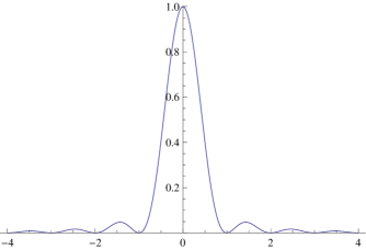
It is easy to see that the global maximum is at $x=0$ and that $\psi(x)$ is decreasing up to $x=1/\sigma$, proving the claim for any $\tau\leq 1/\sigma$ (though the bound worsens as $\tau$ approaches $1/\sigma$ as $\psi(1/\sigma)=0$). ∎

Proof of the Random Matrix Theory prediction in Theorem 1.3.

We assume the conjectures from Random Matrix Theory hold for any even test function, and not just Schwartz test functions. We therefore take $\phi(x)$ to be the characteristic function of the interval $[-\tau,\tau]$, which has Fourier transform equal to $\frac{\sin(2\pi\tau y)}{2\pi\tau y}\cdot 2\tau$. Using such a test function simply counts all normalized zeros in our family that are in $[-\tau,\tau]$ (there is no weighting as $\phi$ is identically 1 in this interval). Thus the predicted average number of such zeros in this interval as $R\to\infty$ is

$$\int_{-\infty}^{\infty}\mathaccent 866{\phi}(y)\mathaccent 866{W}_{r;{\rm SO}}(y)dy \ =\ \int_{-\infty}^{\infty}\mathaccent 866{\phi}(y)\left(\delta(y)+\frac{1}{2}+r\right)dy$$ (3.14)

$$= \left(r+\frac{1}{2}\right)\phi(0)+\mathaccent 866{\phi}(0)$$

$$= r+\frac{1}{2}+2\tau.$$

∎

3.3. Explicit upper and lower bounds

We conclude by determining the upper and lower bounds from Theorem 1.3 for the average number of normalized zeros in given intervals as $R\to\infty$.

We first consider the lower bound, which means we must maximize $C(h)$ (as it is in the denominator for $\tau$, the larger $C(h)$ the smaller the window). As the optimal choice of $h$ (in a given class of functions) is only slightly better than similar $h$, we do not spend too much time on determining the truly best $h$. Consider the family of functions given by

$$h_{n}(x)\ =\ (1-x^{2})(1+a_{2}x^{2}+\dots+a_{2i}x^{2i}+\dots+a_{2n}x^{2n}).$$ (3.15)

We set $a_{0}=1$ as the maximum is to occur at $x=0$, and since the ratio is invariant under rescaling the $a_{i}$’s, we might as well take $a_{0}=1$. Note that each $a_{2i+1}=0$ as our function is even. We chose $h_{n}$ of this form as this forces $h_{n}$ to be even and to vanish at $\pm 1$. We have

$$C(h_{n})\ =\ \left(-\frac{\int_{0}^{1}h_{n}(u)^{2}du}{\int_{0}^{1}h_{n}(u)h_{n}^{\prime\prime}(u)du}\right)^{1/2}.$$ (3.16)

The optimum value of the square-root appears to be $2/\pi$. For example, when $n=2$ we must compute

$$\max_{a_{2},a_{4}}\left(-\frac{\frac{8}{15}+\frac{16a_{2}}{105}+\frac{8a_{2}^{2}}{315}+\frac{16a_{4}}{315}+\frac{16a_{2}a_{4}}{693}+\frac{8a_{4}^{2}}{1287}}{-\frac{4}{3}-\frac{8a_{2}}{15}-\frac{44a_{2}^{2}}{105}-\frac{8a_{4}}{35}-\frac{8a_{2}a_{4}}{15}-\frac{52a_{4}^{2}}{231}}\right)^{1/2}$$ (3.17)

$$\ =\ \max_{a_{2},a_{4}}\left(\frac{6006+286a_{2}^{2}+572a_{4}+70a_{4}^{2}+52a_{2}(33+5a_{4})}{39(385+121a_{2}^{2}+66a_{4}+65a_{4}^{2}+154a_{2}(1+a_{4}))}\right)^{1/2};$$

this is the quantity inside the square-root, not $C(h)$. Using Mathematica we find the optimal values are $a_{2}\approx-.233428$ and $a_{4}\approx.0189588$, which leads to $C(h)\approx 0.63662$; as $2/\pi\approx 0.63662$, this suggests the optimal value of $C(h)$ might be $2/\pi$. This yields the window $\left(-\frac{1}{2\sigma},\frac{1}{2\sigma}\right)$ in which we have on average (as $R\to\infty$) $r+\frac{1}{2}$ zeros.

Remark 3.4.

As we expect the true answer to be a window of size $0$ (i.e., we expect to be able to take $\sigma=\infty$), it is not worthwhile to find the true optimum above merely to save a bit in a few decimal places. The purpose of this analysis is to show that we do see the correct number of zeros on average in the limit in a window of size proportional to $1/\sigma$; the actual value of the proportionality constant, while interesting, is in some sense immaterial as we believe the density conjecture holds for arbitrary $\sigma$.

We list some approximate values for $C(h)$ for other obvious candidates, which are all less than the 0.63662 (which is approximately $2/\pi$) found above.

• $h(x)=(1-x^{2})^{2}$ has $C(h)\approx 0.57735$ (with the quantity inside the square-root looking like $1/3$); if we take just $(1-x^{2})$ we get $C(h)=\sqrt{2/5}\approx 0.632456$.

• $h(x)=\exp(-1/(1-x^{2}))$ has $C(h)\approx 0.570024$.

• $h(x)=\exp(-.754212/(1-x^{2}))$ has $C(h)\approx 0.575629$ (the value of $.754212$ was obtained by searching for optimal test functions among $\exp(-a/(1-x^{2}))$).

We now turn to finding explicit upper bounds for the average number of normalized zeros in $[-\tau,\tau]$ as $R\to\infty$. We continue to analyze the candidate function $\psi(x)=\left(\frac{\sin(\pi\sigma x)}{\pi\sigma x}\right)^{2}$ (see Figure 2 for a plot). We have freedom in terms of how we rate our approximation; for example, we can decrease the upper bound if we simultaneously decrease the size of the interval.

A natural value to take for the size of our interval is the optimal interval found in the lower bound analysis, namely set $\tau\approx 1/2\sigma$. As

$$\mathaccent 866{\psi}(y)\ =\ \begin{cases}\frac{1}{\sigma}\left(1-\frac{|y|}{\sigma}\right)&\text{if $|y|\leq\sigma$}\\ 0&\text{otherwise,}\end{cases}$$ (3.18)

we have $\mathaccent 866{\psi}(0)=1/\sigma$, $\psi(0)=1$ and $\psi(1/2\sigma)=4/\pi^{2}\approx 0.810569$ (or if we believe the approximations, $\psi(\tau)=\frac{\pi^{2}}{4}\sin^{2}(2/\pi)$). Thus after some algebra we see that the average number of normalized zeros in the interval $(-\frac{1}{2\sigma},\frac{1}{2\sigma})$ is at most $\frac{\pi^{2}}{4}\left(r+\frac{1}{2}+\frac{1}{\sigma}\right)$.

Appendix A Standard Conjectures

At various points in the paper we assume the following conjectures.

Generalized Riemann Hypothesis (for Elliptic Curves). Let $\Lambda(s,E)$ be the completed, normalized $L$-function of an elliptic curve $E$ with function equation $s\to 1-s$. The non-trivial zeros $\rho$ of $\Lambda(s,E)$ have $\mbox{Re}(\rho)=1/2$.

Birch and Swinnerton-Dyer Conjecture [BS-D1, BS-D2]. Let $E$ be an elliptic curve of geometric rank $r$ over $\mathbb{Q}$ with Mordell-Weil group $E(\mathbb{Q})=\mathbb{Z}^{r}\oplus\mathbb{T}$. Then the analytic rank (the order of vanishing of the completed $L$-function at the critical point) equals the geometric rank.

Tate’s Conjecture for Elliptic Surfaces [Ta]. Let $\mathcal{E}/\mathbb{Q}$ be an elliptic surface and $L_{2}(\mathcal{E},s)$ be the $L$-series attached to $H^{2}_{\mbox{{\'{e}}t}}(\mathcal{E}/\overline{\mathbb{Q}},\mathbb{Q}_{l})$. $L_{2}(\mathcal{E},s)$ has a meromorphic continuation to $\mathbb{C}$ and $-\mbox{ord}_{s=1}L_{2}(\mathcal{E},s)$ $=\mbox{rank}\ NS(\mathcal{E}/\mathbb{Q})$, where $NS(\mathcal{E}/\mathbb{Q})$ is the $\mathbb{Q}$-rational part of the Néron-Severi group of $\mathcal{E}$. Further, $L_{2}(\mathcal{E},s)$ does not vanish on the line $\mbox{Re}(s)=1$.

Remark A.1.

Tate’s conjecture is known for rational elliptic surfaces. An elliptic surface $\mathcal{E}:y^{2}=x^{3}+A(T)x+B(T)$ is rational if and only if one of the following is true: $(1)$ $0<\max\{3\ {\rm deg}A,2\ {\rm deg}B\}<12;$ $(2)$ $3\ {\rm deg}A=2\ {\rm deg}B=12$ and ${\rm ord}_{T=0}T^{12}\Delta(T^{-1})=0$. See [RSi], pages $46-47$ for more details.

ABC Conjecture. Fix $\epsilon>0$. For co-prime positive integers $a$, $b$ and $c$ with $c=a+b$ and $N(a,b,c)=\prod_{p|abc}p$, $c\ll_{\epsilon}N(a,b,c)^{1+\epsilon}$.

The full strength of ABC is never needed; rather, we need a consequence of ABC, the Square-Free Sieve Conjecture (see [Gr]):

Square-Free Sieve Conjecture. Fix an irreducible polynomial $f(t)$ of degree at least $4$. As $N\to\infty$, the number of $t\in[N,2N]$ with $f(t)$ divisible by $p^{2}$ for some $p>\log N$ is $o(N)$.

For irreducible polynomials of degree at most $3$, the above is known, complete with a better error than $o(N)$ ([Ho], chapter $4$).

We use the Square-Free Sieve to handle the variations in the conductors. If our evaluation of the logarithm of the conductors is off by as little as a small constant, the prime sums become untractable. This is why many works normalize by the average log-conductor.

The following conjecture is used only to interpret some of our results (unless we are calculating the 2-level density to distinguish the three orthogonal candidate groups).

Restricted Sign Conjecture (for the Family $\mathcal{F}$). Consider a one-parameter family $\mathcal{F}$ of elliptic curves. As $N\to\infty$, the signs of the curves $E_{t}$ are equidistributed for $t\in[N,2N]$.

The Restricted Sign conjecture can fail (there are families with constant $j(E_{t})$ where all curves have the same sign, as well as more exotic examples). Helfgott [He] has related the Restricted Sign conjecture to the Square-Free Sieve conjecture and standard conjectures on sums of Moebius:

Polynomial Moebius. Let $f(t)$ be a non-constant polynomial such that no fixed square divides $f(t)$ for all $t$. Then $\sum_{t=N}^{2N}\mu(f(t))=o(N)$.

The Polynomial Moebius conjecture is known for linear $f(t)$.

Helfgott shows the Square-Free Sieve and Polynomial Moebius imply the Restricted Sign conjecture for many families; this is also discussed in [Mil1]. More precisely, let $M(t)$ be the product of the irreducible polynomials dividing $\Delta(t)$ and not $c_{4}(t)$.

Theorem: Equidistribution of Sign in a Family [He]: Let $\mathcal{F}$ be a one-parameter family with $a_{i}(t)\in\mathbb{Z}[t]$. If $j(E_{t})$ and $M(t)$ are non-constant, then the signs of $E_{t}$, $t\in[N,2N]$, are equidistributed as $N\to\infty$. Further, if we restrict to good $t$, $t\in[N,2N]$ such that $D(t)$ is good (usually square-free), the signs are still equidistributed in the limit.