A Case for Hidden $\mathbf{b\bar{b}}$ Tetraquarks based on $\mathbf{e^{+}e^{-}\to b\bar{b}}$ Cross Section between $\sqrt{s}=10.54$ and $\mathbf{1}1.20$ GeV

Abstract

We study the spectroscopy and dominant decays of the bottomonium-like tetraquarks (bound diquarks-antidiquarks), focusing on the lowest lying P-wave $[bq][\bar{b}\bar{q}]$ states $Y_{[bq]}$ (with $q=u,d$), having $J^{PC}=1^{--}$. To search for them, we analyse the BaBar data :2008hx obtained during an energy scan of the $e^{+}e^{-}\to b\bar{b}$ cross section in the range of $\sqrt{s}=10.54$ to 11.20 GeV. We find that these data are consistent with the presence of an additional $b\bar{b}$ state $Y_{[bq]}$ with a mass of 10.90 GeV and a width of about 30 MeV apart from the $\Upsilon(5S)$ and $\Upsilon(6S)$ resonances. A closeup of the energy region around the $Y_{[bq]}$-mass may resolve this state in terms of the two mass eigenstates, $Y_{[b,l]}$ and $Y_{[b,h]}$, with a mass difference, estimated as about 6 MeV. We tentatively identify the state $Y_{[bq]}(10900)$ from the $R_{b}$-scan with the state $Y_{b}(10890)$ observed by Belle Abe:2007tk in the process $e^{+}e^{-}\to Y_{b}(10890)\to\Upsilon(1S,2S)\;\pi^{+}\pi^{-}$ due to their proximity in masses and decay widths.

I Introduction

In the past several years, experiments at the two B-factories, BaBar and Belle, and at the Tevatron collider, CDF and D0, have discovered an impressive number of new hadronic states in the mass region of the charmonia Amsler:2008zzb . These states generically labelled as $X$, $Y$ and $Z$, however, defy a conventional $c\bar{c}$ charmonium interpretation  Jaffe:2004ph ; Quigg:2004vf . Moreover, they are quite numerous, with some 14 of them discovered by the last count, ranging in mass from the $J^{PC}=1^{++}$ $X(3872)$, decaying into $D\bar{D}^{*},J/\psi\pi^{+}\pi^{-},J\psi\gamma$, to the $J^{PC}=1^{--}$ $Y(4660)$, decaying into $\psi^{\prime}\pi^{+}\pi^{-}$ (for a recent experimental summary and references, see  Zupanc:2009qc ). There is also evidence for an $s\bar{s}$ bound state, $Y_{s}(2175)$ having the quantum numbers $J^{PC}=1^{--}$, first observed by BaBar in the initial state radiation (ISR) process $e^{+}e^{-}\to\gamma_{\rm ISR}\;f_{0}(980)\phi(1020)$, where $f_{0}(980)$ is the $0^{++}$ scalar state Aubert:2006bu . This was later confirmed by BES :2007yt and Belle Shen:2009zze .

These states are the subject of intense phenomenological studies. Three different frameworks have been suggested to accommodate them: (i) $D-D^{\ast}$ molecules Tornqvist:2004qy ; Liu:2005ay ; Rosner:2007mu ; (ii) $c\bar{c}g$ hybrids Kou:2005gt ; and (iii) Diquark-antidiquark or four quark states Maiani:2004vq ; Maiani:2005pe ; Drenska:2008gr . Of these hypotheses (i) and (iii) are more popular. For example, the motivation to explain the state $X\left(3872\right)$, first observed by Belle Choi:2003ue and later confirmed by CDF Acosta:2003zx , D0 Abazov:2004kp and BaBar Aubert:2004ns , as a hadronic molecule is that the mass of this state is very close to the $D^{0}\bar{D}^{\ast 0}$ threshold. Hence, in this picture, the binding energy is small implying that these are not compact hadrons, which have typical sizes of $O(1)$ Fermi. This makes it unlikely that such a loosely bound state could be produced promptly (i.e. not from $B$ decays, as seen by Belle and BaBar) in high energy hadron collisions, unless one tailors the wave functions to avoid this conclusion. In particular, Bignamini et al. Bignamini:2009sk have estimated the prompt production cross section of $X\left(3872\right)$ at the Tevatron, assuming it as a $D^{0}\bar{D}^{\ast 0}$ hadron molecule. Their upper bound on the cross section $p\bar{p}\to X(3872)+...$ is about two orders of magnitude smaller than the minimum production cross section from the CDF data Abulencia:2006ma , disfavouring the molecular interpretation of $X(3872)$. However, a dissenting estimate Artoisenet:2009 yields a much larger cross section, invoking the charm meson rescatterings.

The case that the $X,Y,Z$ and $Y_{s}$ are diquark-antidiquark hadrons, in which the diquark (antidiquark) pairs are in colour $\bar{3}_{c}$ ($3_{c}$) configuration bound together by the QCD colour forces, has been forcefully made by Maiani, Polosa and their collaborators Maiani:2004vq ; Maiani:2005pe ; Drenska:2008gr . The idea itself that diquarks in this colour configuration can play a fundamental role in hadron spectroscopy is rather old, going back well over thirty years to the suggestions by Jaffe Jaffe:1976ih . More recently, diquarks were revived by Jaffe and Wilczek Jaffe:2003sg in the context of exotic hadron spectroscopy, in particular, pentaquark baryons (antidiquark-antidiquark-quark), which now seem to have receded into oblivion. However, diquarks as constituents of hadronic matter may (eventually) find their rightful place in particle physics. Lately, interest in this proposal has re-emerged, with a well-founded theoretical interpretation of the low lying scalar mesons as dominantly diquark-antidiquark states and the ones lying higher in mass in the 1 - 2 GeV region as being dominantly $q\bar{q}$ mesons Hooft:2008we . Evidence in favour of an attractive diquark (antidiquark) $qq$ channel for the so-called good diquarks (colour antitriplet $\bar{3}_{c}$, flavour antisymmetric $\bar{3}_{f}$, spin-singlet positive parity) in the characterisation of Jaffe Jaffe:2004ph is now also emerging from more than one Lattice QCD studies Alford:2000mm ; Alexandrou:2006cq for the light quark systems. On the other hand, no evidence is found on the lattice for an attractive diquark channel for the so-called bad diquarks (i.e., spin-1 states) involving light quarks Alexandrou:2006cq . However, as the effective QCD Lagrangian is spin-independent in the heavy quark limit, we anticipate that also the bad diquarks will be found to be in attractive channel for the $[cq]$ and $[bq]$ diquarks having a charm or a beauty quark. This implies a huge number of heavy tetraquark states, as we also show here for the hidden $b\bar{b}$ tetraquark spectroscopy. Earlier work along these lines has been reported in the literature using relativistic quark models Ebert:2008se and QCD sum rules Wang:2009kw .

In this paper, we study the tetraquark picture in the bottom ($b\bar{b}$) sector. In the first part (Section II), we classify these states according to their $J^{PC}$ quantum numbers and calculate the mass spectrum of the diquarks-antidiquarks $[bq][\bar{b}\bar{q}^{\prime}]$ with $q$, $q^{\prime}=u$, $d$, $s$ and $c$ in the ground and orbitally excited states by assuming both good and bad diquarks. The resulting mass spectrum for the $0^{++},1^{++},1^{+-},1^{--}$ and $2^{++}$ states having the valence diquark-antidiquark content $[bq][\bar{b}\bar{q}]$, with $q=u,d,s$ and $c$, and the mixed ones $[bd][\bar{b}\bar{s}]$ (and charge conjugates) is shown in Fig. 1. The main focus of this letter is on the $J^{PC}=1^{--}$ states, which are excited $P$-wave states. To be specific, there are four neutral states $Y_{[bu]}^{(n)}$ $(n=1,...,4)$ with the quark content $([bu][\bar{b}\bar{u}])$ (which differ in their spin assignments) and another four $Y_{[bd]}^{(n)}$ with the quark content $([bd][\bar{b}\bar{d}])$. In the isospin symmetry limit, which is used in calculating the entries in Fig. 1, these mass states are degenerate for each $n$. Isospin-breaking introduces a mass splitting and the mass eigenstates called $Y^{(n)}_{[b,l]}$ and $Y^{(n)}_{[b,h]}$ (for lighter and heavier of the two) become linear combinations of $Y_{[bu]}^{(n)}$ and $Y_{[bd]}^{(n)}$. Thus, $Y^{(n)}_{[b,l]}\equiv\cos\theta\;Y^{(n)}_{[bu]}+\sin\theta\;Y^{(n)}_{[bd]}$ and $Y^{(n)}_{[b,h]}\equiv-\sin\theta\;Y^{(n)}_{[bu]}+\cos\theta\;Y^{(n)}_{[bd]}$. The mass differences are estimated to be small, with $M(Y^{(n)}_{[b,h]})-M(Y_{[b,l]})=(7\pm 2)\cos 2\theta$ MeV, where $\theta$ is a mixing angle. The electromagnetic couplings of the tetraquarks $Y^{(n)}_{[b,l]}$ and $Y^{(n)}_{[b,h]}$ are calculated assuming that the diquarks have point-like couplings with the photon, given by $eQ_{[bq]}$ where $e^{2}/(4\pi)$ is the electromagnetic fine structure constant $\alpha$ and $Q_{[bq]}=+1/3$ for the $[bu]$ and $[bc]$ diquarks and $Q_{[bq]}=-2/3$ for the $[bd]$ and $[bs]$ diquarks. Because of this charge assignment, electromagnetic couplings of the tetraquarks $Y^{(n)}_{[b,l]}$ and $Y^{(n)}_{[b,h]}$ will depend on the mixing angle $\theta$ (Section III).

To calculate the production cross sections $e^{+}e^{-}\to Y^{(n)}_{[b,l]}\to{\rm hadrons}$ and $e^{+}e^{-}\to Y^{(n)}_{[b,h]}\to{\rm hadrons}$, we need to calculate the partial widths $\Gamma^{(n)}_{ee}(Y_{[b,l]})$ and $\Gamma^{(n)}_{ee}(Y_{[b,h]})$ for decays into $e^{+}e^{-}$ pair and the hadronic decay widths $\Gamma(Y^{(n)}_{[b,l]})$ and $\Gamma(Y^{(n)}_{[b,h]})$. For the $\Upsilon(nS)$, the leptonic decay widths are determined by the wave functions at the origin $\Psi_{b\bar{b}}(0)$. The tetraquark states $Y^{(n)}_{[b,l]}$ and $Y^{(n)}_{[b,h]}$ are P-wave states, and we need the derivative of the corresponding wave functions at the origin, $\Psi^{\prime}_{b\bar{b}}(0)$. To take into account the possibly larger hadronic size of the tetraquarks compared to that of the $b\bar{b}$ mesons, we modify the Quarkonia potential, usually taken as a sum of linear (confining) and Coulombic (short-distance) parts. For example, the Buchmüller-Tye $Q\bar{Q}$ potential Buchmuller:1980su has the asymptotic forms $V(r)\sim k_{Q\bar{Q}}\;r$ (for $r\to\infty$) and $V(r)\sim 1/r\ln(1/\Lambda_{\rm QCD}^{2}\;r^{2})$ (for $r\to 0$), where $k_{Q\bar{Q}}$ is the string tension and $\Lambda_{\rm QCD}$ is the QCD scale parameter. The bound state tetraquark potential $V_{\cal Q\bar{\cal Q}}(r)$ will differ from the Quarkonia potential $V_{Q\bar{Q}}(r)$ in the linear part, as the string tension in a diquark $k_{\cal Q\cal Q}$ is expected to be different than the corresponding string tension $k_{Q\bar{Q}}$ in the $Q\bar{Q}$ mesons, but as the diquarks-antidiquarks in the tetraquarks and the quarks-antiquarks in the mesons are in the same ($\bar{3}_{c}3_{c}$) colour configuration, the Coulomb (short-distance) parts of the potentials will be similar. Defining $\kappa=k_{\cal Q\bar{\cal Q}}/k_{Q\bar{Q}}$, we expect $\kappa$ to have a value in the range $\kappa\in[\frac{1}{2},\frac{\sqrt{3}}{2}]$ Alexandrou:2006cq . A value of $\kappa$ different from unity will modify the tetraquark wave functions $\Psi_{\cal Q\bar{\cal Q}}(0)$ from the corresponding ones of the bound $b\bar{b}$ systems, effecting the leptonic decay widths of the tetraquarks. Hadronic decays of $Y^{(n)}_{[b,l]}$ and $Y^{(n)}_{[b,h]}$ are calculated by relating them to the corresponding decays of the $\Upsilon(5S)$, such as $\Upsilon(5S)\to B^{(*)}\bar{B}^{(*)}$, which we take from the PDG. We assume that the form factors in the two set of decays $(Y_{[b,q]}$ and $\Upsilon(5S)$) are related by $\kappa$, yielding the hadronic decay widths (Section IV).

Having specified the mass spectrum and our dynamical assumptions for the tetraquark decays, we undertake a theoretical analysis of the existing data from BaBar :2008hx on $R_{b}(s)=\sigma(e^{+}e^{-}\to b\bar{b})/\sigma(e^{+}e^{-}\to\mu^{+}\mu^{-})$, obtained during an energy scan of the $e^{+}e^{-}\to b\bar{b}$ cross section in the range of $\sqrt{s}=10.54$ to 11.20 GeV. The question that we ask and try to partially answer is: Are the kinematically allowed tetraquark states $Y^{(n)}_{[b,h]}$ and $Y^{(n)}_{[b,l]}$ visible in the BaBar energy scan of $R_{b}$? To that end, we calculate the contributions of the lowest $1^{--}$ tetraquark states $Y_{[b,h]}$ and $Y_{[b,l]}$ to the hadronic cross sections $\sigma(e^{+}e^{-}\to Y_{[b,l]}\to\;{\rm hadrons})$ and $\sigma(e^{+}e^{-}\to Y_{[b,h]}\to\>{\rm hadrons})$, and hence the corresponding contributions $\Delta R_{b}(s)$. Our fits of the BaBar $R_{b}$-data are consistent with the presence of a single state $Y_{[bq]}$ as a Breit-Wigner resonance with the mass around $10.90$ GeV and a width of about $30$ MeV, in addition to the $\Upsilon(5S)$ and $\Upsilon(6S)$. The quality of the fit with three Breit-Wigners is found to be better than the one obtained with just 2 (i.e., with $\Upsilon(5S)$ and $\Upsilon(6S)$), as reported by BaBar :2008hx (Section V). A closeup of the energy region around 10.90 GeV is necessary to confirm and resolve the structure reported by us, as the isospin-induced mass difference between the two eigenstates $Y_{[b,h]}$ and $Y_{[b,l]}$ comes out as about 6 MeV, which is comparable to the BaBar centre-of-mass energy step of 5 MeV. We hope that this can be investigated in the near future by Belle.

We tentatively identify the state $Y_{[bq]}(10900)$ with the state $Y_{b}(10890)$ measured in the process $e^{+}e^{-}\to Y_{b}(10890)\to\Upsilon(1S,2S)\;\pi^{+}\pi^{-}$ Abe:2007tk . An analysis Ali:2009es of the Belle data on the decay widths $\Gamma(Y_{b}\to\Upsilon(1S,2S)\;\pi^{+}\pi^{-})$, dipion invariant mass spectra and the helicity angular distributions is in agreement with the tetraquark interpretation presented here.

II Spectrum of bottom diquark-antidiquark states

The mass spectrum of tetraquarks $[bq][\overline{bq^{\prime}]}$ with $q=u$, $d$, $s$ and $c$ can be described in terms of the constituent diquark masses, $m_{\cal Q}$, spin-spin interactions inside the single diquark, spin-spin interaction between quark and antiquark belonging to two diquarks, spin-orbit, and purely orbital term Drenska:2008gr , i.e.

$$H=2m_{\cal Q}+H_{SS}^{(\cal Q\cal Q)}+H_{SS}^{(\cal Q\bar{\cal Q}\mathcal{)}}+H_{SL}+H_{LL},$$ (1)

where:

$$H_{SS}^{(\cal Q\cal Q)} = 2(\mathcal{K}_{bq})_{\bar{3}}[(\mathbf{S}_{b}\cdot\mathbf{S}_{q})+(\mathbf{S}_{\bar{b}}\cdot\mathbf{S}_{\bar{q}})],$$

$$H_{SS}^{(\cal Q\bar{\cal Q}\mathcal{)}} = 2(\mathcal{K}_{b\bar{q}})(\mathbf{S}_{b}\cdot\mathbf{S}_{\bar{q}}+\mathbf{S}_{\bar{b}}\cdot\mathbf{S}_{q})+2\mathcal{K}_{b\bar{b}}(\mathbf{S}_{b}\cdot\mathbf{S}_{\bar{b}})+2\mathcal{K}_{q\bar{q}}(\mathbf{S}_{q}\cdot\mathbf{S}_{\bar{q}}),$$

$$H_{SL} = 2A_{\cal Q}(\mathbf{S}_{\mathcal{Q}}\cdot\mathbf{L}+\mathbf{S}_{\mathcal{\bar{Q}}}\cdot\mathbf{L}),$$

$$H_{LL} = B_{\cal Q}\frac{L_{\cal Q\bar{\cal Q}}(L_{\cal Q\bar{\cal Q}}+1)}{2}.$$ (2)

Here $m_{\cal Q}$ is the mass of the diquark $[bq]$, $(\mathcal{K}_{bq})_{\bar{3}}$ is the spin-spin interaction between the quarks inside the diquarks, $\mathcal{K}_{b\bar{q}}$ are the couplings ranging outside the diquark shells, $A_{\cal Q}$ is the spin-orbit coupling of diquark and $B_{\cal Q}$ corresponds to the contribution of the total angular momentum of the diquark-antidiquark system to its mass. The overall factor of $2$ is used customarily in the literature. For the calculation of the masses we assume isospin symmetry, i.e. the isodoublet consisting of the states

$$Y^{(n)}_{[bu]}=[bu][\bar{b}\bar{u}]\enspace\enspace\enspace\textnormal{and}\enspace\enspace\enspace Y^{(n)}_{[bd]}=[bd][\bar{b}\bar{d}]$$ (3)

are degenerate in mass for each $n$. Later, we will calculate the isospin symmetry breaking effects in the masses.

The parameters involved in the above Hamiltonian (2) can be obtained from the known meson and baryon masses by resorting to the constituent quark model De Rujula:1975ge

$$H=\sum\limits_{i}m_{i}+\sum\limits_{i<j}2\mathcal{K}_{ij}(\mathbf{S}_{i}\cdot\mathbf{S}_{j}),$$ (4)

where the sum runs over the hadron constituents. The coefficient $\mathcal{K}_{ij}$ depends on the flavour of the constituents $i$, $j$ and on the particular colour state of the pair. Using the entries in the PDG for hadron masses along with the assumption that the spin-spin interactions are independent of whether the quarks belong to a meson or a diquark, the results for diquark masses corresponding to $X\left(3872\right)$ and $Y\left(2175\right)$ were calculated in the literature Maiani:2004vq ; Drenska:2008gr . Here, we extend this procedure to the tetraquarks $[bq][\bar{b}\bar{q}]$. The constituent quark masses and the couplings $\mathcal{K}_{ij}$ for the colour singlet and antitriplet states are given in Table I, II and III.

Table 1: Constituent quark masses derived from the $L=0$ mesons and baryons.

Constituent mass (MeV)	$q$	$s$	$c$	$b$
Mesons	$305$	$490$	$1670$	$5008$
Baryons	$362$	$546$	$1721$	$5050$

Table 2: Spin-Spin couplings for quark-antiquark pairs in the colour singlet state from the known mesons.

Spin-spin couplings	$q\bar{q}$	$s\bar{q}$	$s\bar{s}$	$c\bar{q}$	$c\bar{s}$	$c\bar{c}$	$b\bar{q}$	$b\bar{s}$	$b\bar{c}$	$b\bar{b}$
$\left(\mathcal{K}_{ij}\right)_{0}$(MeV)	$318$	$200$	$129$	$71$	$72$	$59$	$23$	$23$	$20$	$36$

Table 3: Spin-Spin couplings for quark-quark pairs in colour $\bar{3}$ state from the known baryons.

Spin-Spin couplings	$qq$	$sq$	$cq$	$cs$	$ss$	$bq$	$bs$	$bc$
$\left(\mathcal{K}_{ij}\right)_{\bar{3}}$(MeV)	$98$	$65$	$22$	$24$	$72$	$6$	$25$	$10$

To calculate the spin-spin interaction of the $\cal Q\bar{\cal Q}$ states explicitly, we use the non-relativistic notation $\left|S_{\cal Q}\text{,~{}}S_{\bar{\cal Q}};~{}J\right\rangle$, where $S_{\cal Q}$ and $S_{\bar{\cal Q}}$ are the spin of diquark and antidiquark, respectively, and $J$ is the total angular momentum. These states are then defined in terms of the direct product of the $2\times 2$ matrices in spinor space, $\Gamma^{\alpha}$, which can be written in terms of the Pauli matrices as:

$$\Gamma^{0}=\frac{\sigma_{2}}{\sqrt{2}};~{}\Gamma^{i}=\frac{1}{\sqrt{2}}\sigma_{2}\sigma_{i}~{},$$ (5)

which then lead to the following definitions:

$$\left|0_{\cal Q},0_{\bar{\cal Q}};~{}0_{J}\right\rangle = \frac{1}{2}\left(\sigma_{2}\right)\otimes\left(\sigma_{2}\right),$$

$$\left|1_{\cal Q},1_{\bar{\cal Q}};~{}0_{J}\right\rangle = \frac{1}{2\sqrt{3}}\left(\sigma_{2}\sigma^{i}\right)\otimes\left(\sigma_{2}\sigma^{i}\right),$$

$$\left|0_{\cal Q},1_{\bar{\cal Q}};~{}1_{J}\right\rangle = \frac{1}{2}\left(\sigma_{2}\right)\otimes\left(\sigma_{2}\sigma^{i}\right),$$

$$\left|1_{\cal Q},0_{\bar{\cal Q}};~{}1_{J}\right\rangle = \frac{1}{2}\left(\sigma_{2}\sigma^{i}\right)\otimes\left(\sigma_{2}\right),$$

$$\left|1_{\cal Q},1_{\bar{\cal Q}};~{}1_{J}\right\rangle = \frac{1}{2\sqrt{2}}\varepsilon^{ijk}\left(\sigma_{2}\sigma^{j}\right)\otimes\left(\sigma_{2}\sigma^{k}\right).$$ (6)

The properties of these matrices are given in the appendix of ref. Maiani:2004vq . The next step is the diagonalization of the Hamiltonian (1) using the basis of states with definite diquark and antidiquark spin and total angular momentum. There are two different possibilities Maiani:2004vq : Lowest lying $[bq][\bar{b}\bar{q}]$ states $\left(L_{\cal Q\bar{\cal Q}}=0\right)$ and higher mass $[bq][\bar{b}\bar{q}]$ states $\left(L_{\cal Q\bar{\cal Q}}=1\right)$, which we discuss below.

II.1 Lowest lying $[bq][\bar{b}\bar{q}]$ states $\left(L_{\cal Q\bar{\cal Q}}=0\right)$

The states can be classified in terms of the diquark and antidiquark spin, $S_{\cal Q}$ and $S_{\bar{\cal Q}}$, total angular momentum $J$, parity, $P$ and charge conjugation, $C$. Considering both good and bad diquarks and having $L_{\cal Q\bar{\cal Q}}=0$ we have six possible states which are listed below.

i. Two states with $J^{PC}=0^{++}$:

$$\left|0^{++}\right\rangle = \left|0_{\cal Q},0_{\bar{\cal Q}};~{}0_{J}\right\rangle;$$

$$\left|0^{++\prime}\right\rangle = \left|1_{\cal Q},1_{\bar{\cal Q}};~{}0_{J}\right\rangle.$$ (7)

ii. Three states with $J=1$:

$$\left|1^{++}\right\rangle = \frac{1}{\sqrt{2}}\left(\left|0_{\cal Q},1_{\bar{\cal Q}};~{}1_{J}\right\rangle+\left|1_{\cal Q},0_{\bar{\cal Q}};~{}1_{J}\right\rangle\right);$$

$$\left|1^{+-}\right\rangle = \frac{1}{\sqrt{2}}\left(\left|0_{\cal Q},1_{\bar{\cal Q}};~{}1_{J}\right\rangle-\left|1_{\cal Q},0_{\bar{\cal Q}};~{}1_{J}\right\rangle\right);$$

$$\left|1^{+-\prime}\right\rangle = \left|1_{\cal Q},1_{\bar{\cal Q}};~{}1_{J}\right\rangle.$$ (8)

All these states have positive parity as both the good and bad diquarks have positive parity and $L_{\cal Q\bar{\cal Q}}=0$. The difference is in the charge conjugation quantum number, the state $\left|1^{++}\right\rangle$ is even under charge conjugation, whereas $\left|1^{+-}\right\rangle$ and $\left|1^{+-\prime}\right\rangle$ are odd.

iii. One state with $J^{PC}=2^{++}$:

$$\left|2^{++}\right\rangle=\left|1_{\cal Q},1_{\bar{\cal Q}};~{}2_{J}\right\rangle.$$ (9)

Keeping in view that for $L_{\cal Q\bar{\cal Q}}=0$ there is no spin-orbit and purely orbital term, the Hamiltonian (1) takes the form

$$H = 2m_{[bq]}+2(\mathcal{K}_{bq})_{\bar{3}}[(\mathbf{S}_{b}\cdot\mathbf{S}_{q})+(\mathbf{S}_{\bar{b}}\cdot\mathbf{S}_{\bar{q}})]+2\mathcal{K}_{q\bar{q}}(\mathbf{S}_{q}\cdot\mathbf{S}_{\bar{q}})$$ (10)

$$+2(\mathcal{K}_{b\bar{q}})(\mathbf{S}_{b}\cdot\mathbf{S}_{\bar{q}}+\mathbf{S}_{\bar{b}}\cdot\mathbf{S}_{q})+2\mathcal{K}_{b\bar{b}}(\mathbf{S}_{b}\cdot\mathbf{S}_{\bar{b}}).$$

The diagonalisation of the Hamiltonian (10) with the states defined above gives the eigenvalues which are needed to estimate the masses of these states. It is straightforward to see that for the $1^{++}$ and $2^{++}$ states the Hamiltonian is diagonal with the eigenvalues Maiani:2004vq

$$M\left(1^{++}\right) = 2m_{[bq]}-(\mathcal{K}_{bq})_{\bar{3}}+\frac{1}{2}\mathcal{K}_{q\bar{q}}-\mathcal{K}_{b\bar{q}}+\frac{1}{2}\mathcal{K}_{b\bar{b}},$$ (11)

$$M\left(2^{++}\right) = 2m_{[bq]}+(\mathcal{K}_{bq})_{\bar{3}}+\frac{1}{2}\mathcal{K}_{q\bar{q}}+\mathcal{K}_{b\bar{q}}+\frac{1}{2}\mathcal{K}_{b\bar{b}}.$$ (12)

All other quantities are now specified except the mass of the constituent diquark. We take the Belle data Zupanc:2009qc as input and identify the $Y_{b}(10890)$ with the lightest of the $1^{--}$ states, $Y_{[bq]}$, yielding a diquark mass $m_{[bq]}=5.251\;\textnormal{GeV}$. This procedure is analogous to what was done in Maiani:2004vq , in which the mass of the diquark $[cq]$ was fixed by using the mass of $X(3872)$ as input, yielding $m_{[cq]}=1.933$ GeV. Instead, if we use this determination of $m_{[cq]}$ and use the formula $m_{[bq]}=m_{[cq]}+\left(m_{b}-m_{c}\right)$, which has the virtue that the mass difference $m_{c}-m_{b}$ is well determined, we get $m_{[bq]}=5.267\;\textnormal{GeV}$, yielding a difference of $16\;\textnormal{MeV}$. This can be taken as an estimate of the theoretical error on $m_{[bq]}$, which then yields an uncertainty of about 30 MeV in the estimates of the tetraquark masses of interest for us.

The couplings corresponding to the spin-spin interactions have been calculated for the colour singlet and colour antitriplet only. In Eq. (2), however, the quantities $\mathcal{K}_{q\bar{q}}$, $\mathcal{K}_{b\bar{q}}$ and $\mathcal{K}_{b\bar{b}}$ involve both colour singlet and colour octet couplings between the quarks and antiquraks in a $\cal Q\bar{\cal Q}$ system. So for $\mathcal{K}_{b\bar{b}}$ Drenska:2008gr

$$\mathcal{K}_{b\bar{b}}\left([bq][\bar{b}\bar{q}]\right)=\frac{1}{3}\left(\mathcal{K}_{b\bar{b}}\right)_{0}+\frac{2}{3}\left(\mathcal{K}_{b\bar{b}}\right)_{8}~{},$$ (13)

where $\left(\mathcal{K}_{b\bar{b}}\right)_{0}$ is reported in Table II. $\left(\mathcal{K}_{b\bar{b}}\right)_{8}$ can be derived from the one gluon exchange model by using the relation Maiani:2004vq :

$$\left(\mathcal{K}_{b\bar{b}}\right)_{\mathbf{X}}\sim\left(C^{2}\left(\mathbf{X}\right)-C^{2}\left(\mathbf{3}\right)-C^{2}\left(\mathbf{\bar{3}}\right)\right)~{},$$ (14)

with $C^{2}\left(\mathbf{X}\right)=0$, $4/3$, $4/3$, $3$ for $\mathbf{X=0}$, $\mathbf{3}$, $\mathbf{\bar{3}}$, $\mathbf{8}$ respectively. Finally, Eq. (13) gives

$$\mathcal{K}_{b\bar{b}}\left([bq][\bar{b}\bar{q}]\right)=\frac{1}{4}\left(\mathcal{K}_{b\bar{b}}\right)_{0}~{}.$$ (15)

Now, we have all the input parameters to calculate the mass spectrum numerically. Putting everything together the masses for the hidden $b\bar{b}$ tetraquark states $1^{++}$ and $2^{++}$ states are:

$$M\left(1^{++}\right) = 10.504\text{ GeV, for }q=u,~{}d,$$ (16)

$$= 10.849\text{ GeV, for }q=s,$$ (17)

$$= 13.217\text{ GeV, for }q=c,$$ (18)

$$M\left(2^{++}\right) = 10.520\text{ GeV, for }q=u,~{}d,$$ (19)

$$= 10.901\text{ GeV, for }q=s,$$ (20)

$$= 13.239\text{ GeV, for }q=c.$$ (21)

For the corresponding $0^{++}$ and $1^{+-}$ tetraquark states, the Hamiltonian is not diagonal and we have the following $2\times 2$ matrices:

$$M\left(0^{++}\right)=\left(\begin{array}[]{cc}-3(\mathcal{K}_{bq})_{\bar{3}}&\frac{\sqrt{3}}{2}\left(\mathcal{K}_{q\bar{q}}+\mathcal{K}_{b\bar{b}}-2\mathcal{K}_{b\bar{q}}\right)\\ \frac{\sqrt{3}}{2}\left(\mathcal{K}_{q\bar{q}}+\mathcal{K}_{b\bar{b}}-2\mathcal{K}_{b\bar{q}}\right)&(\mathcal{K}_{bq})_{\bar{3}}-\left(\mathcal{K}_{q\bar{q}}+\mathcal{K}_{b\bar{b}}+2\mathcal{K}_{b\bar{q}}\right)\end{array}\right),$$ (22)

$$M\left(1^{+-}\right)=\left(\begin{array}[]{cc}-(\mathcal{K}_{bq})_{\bar{3}}+\mathcal{K}_{b\bar{q}}-\frac{\left(\mathcal{K}_{q\bar{q}}+\mathcal{K}_{b\bar{b}}\right)}{2}&\mathcal{K}_{q\bar{q}}-\mathcal{K}_{b\bar{b}}\\ \mathcal{K}_{q\bar{q}}-\mathcal{K}_{b\bar{b}}&(\mathcal{K}_{bq})_{\bar{3}}-\mathcal{K}_{b\bar{q}}-\frac{\left(\mathcal{K}_{q\bar{q}}+\mathcal{K}_{b\bar{b}}\right)}{2}\end{array}\right).$$ (23)

To estimate the masses of these two states, one has to diagonalise the above matrices. After doing this, the mass spectrum of these $b\bar{b}$ states is shown in Fig. 1.

II.2 Higher mass $[bq][\bar{b}\bar{q}]$ states $\left(L_{\cal Q\bar{\cal Q}}=1\right)$

We now discuss orbital excitations with $L_{\cal Q\bar{\cal Q}}=1$ having both good and bad diquarks. In this paper, we are particularly interested in the $1^{--}$ multiplet. Using the basis vectors defined in reference Drenska:2008gr the mass shift due to the spin-spin interaction terms $H_{SS}$ becomes:

$$\Delta M_{SS}=\left(\begin{array}[]{ccc}-3\left(\mathcal{K}_{bq}\right)_{\bar{3}}&0&0\\ 0&-\left(\mathcal{K}_{bq}\right)_{\bar{3}}-\mathcal{K}_{b\bar{q}}+\left(\mathcal{K}_{q\bar{q}}+\mathcal{K}_{b\bar{b}}\right)/2&0\\ 0&0&-\left(\mathcal{K}_{bq}\right)_{\bar{3}}-\mathcal{K}_{b\bar{q}}-\left(\mathcal{K}_{q\bar{q}}+\mathcal{K}_{b\bar{b}}\right)/2\end{array}\right)~{}.$$ (24)

The eigenvalues of the spin-orbit and angular momentum operators given in Eq. (1) were calculated by Polosa et al. Drenska:2008gr , and we have summarised these values in Table 4.

Table 4: Eigenvalues of the spin-orbit and angular momentum operator in Eq. (1) for the states having $J=L_{\cal Q\bar{\cal Q}}+S_{\cal Q\bar{\cal Q}}=1.$

$\left|S_{\cal Q}\,\text{, }S_{\bar{\cal Q}}\text{, }S_{\cal Q\bar{\cal Q}}\text{, }L_{\cal Q\bar{\cal Q}}\right\rangle$	$a\left(S_{\cal Q}\,\text{, }S_{\bar{\cal Q}}\text{, }S_{\cal Q\bar{\cal Q}}\text{, }L_{\cal Q\bar{\cal Q}}\right)$	$b\left(s_{\cal Q}\,\text{, }S_{\bar{\cal Q}}\text{, }S_{\cal Q\bar{\cal Q}}\text{, }L_{\cal Q\bar{\cal Q}}\right)$
$\left|0\,\text{, }0\text{, }0\text{, }1\right\rangle$	$~{}~{}0$	$1$
$\left|1\,\text{, }0\text{, }1\text{, }1\right\rangle$	$-2$	$1$
$\left|1\,\text{, }1\text{, }2\text{, }1\right\rangle$	$-6$	$1$
$\left|1\,\text{, }1\text{, }1\text{, }1\right\rangle$	$-2$	$1$
$\left|1\,\text{, }1\text{, }0\text{, }1\right\rangle$	$~{}~{}0$	$1$

Hence the eight tetraquark states $[bq][\bar{b}\bar{q}]$ ($q=u,d$) having the quantum numbers $1^{--}$ are:

$$M_{Y_{[bq]}}^{(1)}\left(S_{\cal Q}=0,~{}S_{\bar{\cal Q}}=0,~{}S_{\cal Q\bar{\cal Q}}=0,~{}L_{\cal Q\bar{\cal Q}}=1\right) = 2m_{\left[bq\right]}+\lambda_{1}+B_{\mathcal{\cal Q}},$$

$$M_{Y_{[bq]}}^{(2)}\left(S_{\cal Q}=1,~{}S_{\bar{\cal Q}}=0,~{}S_{\cal Q\bar{\cal Q}}=1,~{}L_{\cal Q\bar{\cal Q}}=1\right) = 2m_{\left[bq\right]}+\Delta+\lambda_{2}-2A_{\cal Q}+B_{\cal Q},$$

$$M_{Y_{[bq]}}^{(3)}\left(S_{\cal Q}=1,~{}S_{\bar{\cal Q}}=1,~{}S_{\cal Q\bar{\cal Q}}=0,~{}L_{\cal Q\bar{\cal Q}}=1\right) = 2m_{\left[bq\right]}+2\Delta+\lambda_{3}+B_{\cal Q},$$ (25)

$$M_{Y_{[bq]}}^{(4)}\left(S_{\cal Q}=1,~{}S_{\bar{\cal Q}}=1,~{}S_{\cal Q\bar{\cal Q}}=2,~{}L_{\cal Q\bar{\cal Q}}=1\right) = 2m_{\left[bq\right]}+2\Delta+\lambda_{3}-6A_{\cal Q}+B_{\cal Q},$$

where $\lambda_{i}(i=1,2,3)$ are the diagonal elements of the matrix $\Delta M_{SS}$ given in Eq. (24). Note that there are 16 electrically neutral self-conjugate $1^{--}$ tetraquark states $Y_{[bq]}^{(n)}$ with the quark contents $[bq][\bar{b}\bar{q}]$, with $q=u,d,s$ or $c$, of which the two corresponding to $[bu][\bar{b}\bar{u}]$ and $[bd][\bar{b}\bar{d}]$, i.e., $Y_{[bu]}^{(n)}$ and $Y_{[bd]}^{(n)}$ are degenerate in mass due to the isospin symmetry. There are yet more electrically neutral $J^{PC}=1^{--}$ states with the mixed light quark content $[bd][\bar{b}\bar{s}]$ and their charge conjugates $[bs][\bar{b}\bar{d}]$. However, these mixed states don’t couple directly to the photons, $Z^{0}$ or the gluon, and are not of immediate interest to us in this paper.

The numerical values of the coefficients corresponding to $A_{\cal Q}$ and $B_{\cal Q}$ are given in Table 4 and are labelled by $a$ and $b$, respectively. The quantity $\Delta$ is the mass difference of the good and the bad diquarks, i.e.

$$\Delta=m_{\cal Q}\left(S_{\cal Q}=1\right)-m_{\cal Q}\left(S_{\cal Q}=0\right).$$ (26)

In order to calculate the numerical values of these states, we have to estimate $\Delta$ which is the only unknown remaining in this calculation. Following Jaffe and Wilczek Jaffe:2004ph , the value of $\Delta$ for diquark $[bq]$ is $\Delta=202$ MeV for $q=u$, $d$, $s$ and $c$ quarks. We recall that we have used the known mesons and baryons to calculate the couplings of the spin-spin interaction and we can extend the same procedure to the $S=1$, $L=(0$, $1$) meson states $B^{\ast}$, $B_{1}\left(5721\right)$, $B_{2}\left(5747\right)$ to calculate the values of $A_{\cal Q}$ and $B_{\mathcal{Q}}$ which are:

$$A_{\cal Q} = 5\text{ MeV, for }q=u\text{, }d,$$

$$A_{\cal Q} = 3\text{ MeV, for }q=s\text{, }c,$$

$$B_{\cal Q} = 408\text{ MeV, for }q=u\text{, }d,$$

$$B_{\cal Q} = 423\text{ MeV, for }q=s,c.$$ (27)

Numerical values of the masses for the states given in Eq. (25) are quoted in Table V. Some of the entries, in particular $M_{{Y}_{[bq]}^{(1)}}$ ($q=u,d,s$), are comparable with the existing ones in refs. Ebert:2008se ; Wang:2009kw .

Finally, the mass spectrum for the tetraquark states $[bq][\bar{b}\bar{q}]$ for $q=u,d,s,c$ with $J^{PC}=0^{++},1^{++},1^{+-},1^{--}$ and $2^{++}$ states is plotted in Fig. 1 in the isospin-symmetry limit. The $b\bar{b}$ tetraquark states with mixed light quark content $[bd][\bar{b}\bar{s}]$ are also shown in this figure. Of these, the $1^{--}$ state $Y^{(1)}_{[bq]}(10.890)$ shown in the upper left frame in Fig. 1 is of central interest to us in this paper.

Table 5: Masses of the $1^{--}$ tetraquark states $M_{{Y}_{[bq]}}^{(n)}$ in GeV as computed from Eqs. (25), (26) and (27). The value $M_{{Y}_{[bq]}^{(1)}}$ (for $q=u,d$) is fixed to be 10.890 GeV, identifying this with the mass of the $Y_{b}$ from Belle Zupanc:2009qc

.

$M_{{Y}_{[bq]}}^{(i)}$	$q=u$, $d$	$q=s$	$q=c$	$q=d$, $\bar{q}=\bar{s}$
$M_{{Y}_{[bq]}^{(1)}}$	$10.890$	$11.218$	$13.618$	$11.054$
$M_{{Y}_{[bq]}^{(2)}}$	$11.130$	$11.479$	$13.841$	$11.281$
$M_{{Y}_{[bq]}^{(3)}}$	$11.257$	$11.646$	$14.025$	$11.476$
$M_{{Y}_{[bq]}}^{(4)}$	$11.227$	$11.629$	$14.009$	$11.453$

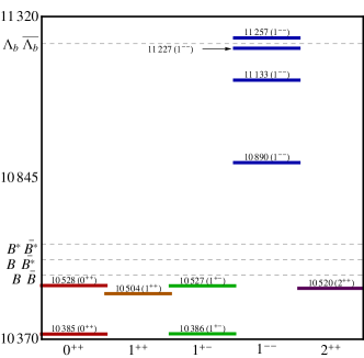
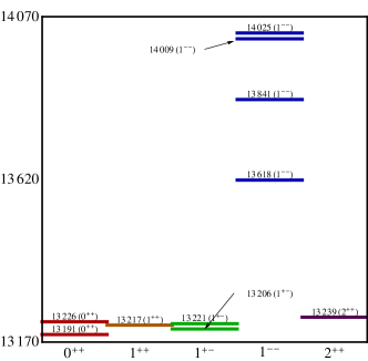
Figure 1: Tetraquark mass spectrum with the valence quark content $[bq][\bar{b}\bar{q}]$ with $q=u,d$, assuming isospin symmetry (upper left frame), with $q=s$ (upper right frame), with $q=c$ (lower left frame), and for the mixed light quark content $[bd][\bar{b}\bar{s}]$ (lower right frame). Some important decay thresholds are indicated by dashed lines. The value 10890 is an input for the lowest $J^{PC}=1^{--}$ tetraquark state $Y_{[bq]}^{(1)}$. All masses are given in MeV.

III Isospin Breaking and Leptonic Decay Widths of the $J^{PC}=1^{--}$ Tetraquarks

We discuss in this section the isospin breaking effects, which were neglected in the previous section, and calculate the decay widths $\Gamma_{ee}(Y_{[b,l]})$ and $\Gamma_{ee}(Y_{[b,h]})$ for $Y_{[b,l]}$ and $Y_{[b,h]}$. The mass eigenstates are given by a linear superposition of the states defined in (3). Introducing a mixing angle $\theta$, we have, for the lighter and heavier states:

$$Y_{[b,l]} = \cos\theta\;Y_{[bu]}+\sin\theta\;Y_{[bd]},$$ (28)

$$Y_{[b,h]} = -\sin\theta\;Y_{[bu]}+\cos\theta\;Y_{bd]}.$$ (29)

The isospin breaking part of the mass matrix is

$$\left(\begin{array}[]{cc}2m_{u}+\delta&\delta\\ \delta&2m_{d}+\delta\end{array}\right),$$ (30)

where $\delta$ is the contribution from quark annihilation diagrams, where the light quark pair annihilates to intermediate gluons. Taking this into account, the isospin mass breaking is given by

$$M(Y_{[b,h]})-M(Y_{[b,l]})=(7\pm 3)\;\cos(2\theta)\;{\rm MeV}.$$ (31)

The partial electronic widths $\Gamma_{ee}(Y_{[b,l]})$ and $\Gamma_{ee}(Y_{[b,h]})$ are given by the well-known Van Royen-Weisskopf formula for the P-states, which we write generically as:

$$\Gamma_{ee}=\frac{16\pi Q^{2}\alpha^{2}|\Psi_{\cal Q\bar{\cal Q}}^{\prime}(0)|^{2}}{M^{2}\omega^{2}},$$ (32)

where $Q=Q_{[bd]}=-2/3$ is the diquark charge in $Y_{bd}=[bd][\bar{b}\bar{d}]$ and $Q=Q_{[bu]}=+1/3$ is the charge of the diquarks in $Y_{bu}=[bu][\bar{b}\bar{u}]$, and $\Psi_{\cal Q\bar{\cal Q}}^{\prime}(\vec{r})=\psi(\phi,\theta)R^{\prime}(r)$ is the first derivative in $r$ of the wave function of the tetraquark, which needs to be taken at the origin, i.e. $\Psi_{\cal Q\bar{\cal Q}}^{\prime}(0)=\sqrt{3/(4\pi)}R^{\prime}(0)$. We have approximated $\omega$ by the diquark mass.

We determine the wave functions for the P-state tetraquarks $[bd][\bar{b}\bar{d}]$ and $[bu][\bar{b}\bar{u}]$ from the corresponding wave functions for the P-state $b\bar{b}$ system by scaling the string tension in the linear part of the potential, as discussed in the introduction. As most potential models agree in their linear (confining) parts Buchmuller:1980su and the linear part of the potential essentially determines the heavy Quarkonia wave functions, the uncertainty in $\Psi_{b\bar{b}}(0)$ from the underlying model is not a concern. We have used the QQ-onia package of DomenechGarret:2008sr , yielding $|R^{\prime}(0)|^{2}=2.062\enspace GeV^{5}$ for the $b\bar{b}$ radial wave function, which we have used as normalisation. The corresponding value for the tetraquark states $[bq][\bar{b}\bar{q}]$ is then calculated as $\Psi_{\cal Q\bar{\cal Q}}(0)\simeq\kappa\Psi_{b\bar{b}}(0)$, and used in our derivations of the decay widths. We expect that for all the P-states $Y^{(n)}_{[bu]}$ and $Y^{(n)}_{[bd]}$, the electronic widths will be constant, to a good approximation.

The ratio ${\mathcal{R}}_{ee}(Y_{b})$ of $\Gamma_{ee}(Y_{[b,l]})$ and $\Gamma_{ee}(Y_{[b,h]})$ is given by

$${\mathcal{R}}_{ee}(Y_{b})\equiv\frac{\Gamma_{ee}(Y_{[b,l]})}{\Gamma_{ee}(Y_{[b,h]})}=\frac{Q_{l}^{2}(\theta)}{Q_{h}^{2}(\theta)}=\left[\frac{1-2\tan\theta}{2+\tan\theta}\right]^{2}~{},$$ (33)

where $Q_{l}(\theta)=Q_{[bu]}\cos\theta+Q_{[bd]}\sin\theta$ and $Q_{h}(\theta)=-Q_{[bu]}\sin\theta+Q_{[bd]}\cos\theta$ are the mixing-angle weighted charges. Since the total cross sections for $e^{+}e^{-}\to(Y_{[b,l]},Y_{[b,h]})\to{\rm hadrons}$ are directly proportional to $\Gamma_{ee}(Y_{[b,l]})$ and $\Gamma_{ee}(Y_{[b,h]})$, the ratio ${\mathcal{R}}_{ee}(Y_{b})$ is accessible from the experiment. The absolute values of the decay widths $\Gamma_{ee}(Y_{[b,l]})$ and $\Gamma_{ee}(Y_{[b,h]})$ are given by $\Gamma_{ee}(Y_{[b,i]})=0.4\;\kappa^{2}Q_{i}(\theta)^{2}$ keV, where $Q_{i}(\theta)$ are the mixing angle weighted charges of the two mass eigenstates, $Y_{[b,l]}$ and $Y_{[b,h]}$. which can also be seen in (33).

IV Diquark-antidiquark decay modes

In this section we discuss the dominant hadronic decays of the $L_{\cal Q\bar{\cal Q}}=1$ states. In doing this, we restrict ourselves to the two-body decays, $Y_{[bq]}\to B_{q}^{(*)}\bar{B}_{q}^{(*)}$, and when allowed kinematically, also the decay $Y_{[bq]}\to\Lambda_{b}\bar{\Lambda}_{b}$. Their thresholds are pictured in figure 1. These decays are Zweig allowed and involve essentially quark rearrangements and the possible pop-up of a light $q\bar{q}$ pair to make the $\Lambda_{b}\bar{\Lambda}_{b}$ state. The decays $Y_{[bq]}\to\Upsilon(1S,2S)\;\pi^{+}\pi^{-}$ are also Zweig allowed. However, they are sub-dominant and can be neglected in estimating the total decay widths.

The vertices and the corresponding decay widths of the dominant decays are given below:

$$\large\begin{array}[]{rclrcl}\raisebox{-30.0pt}{\includegraphics[width=130.08731pt]{VertexDiquarkBBbar.eps}}&\widehat{=}&F(k^{\mu}-l^{\mu})&\Longrightarrow\;\;\Gamma&=&\frac{F^{2}|\vec{k}|^{3}}{2M^{2}\pi},\\ \raisebox{-30.0pt}{\includegraphics[width=117.07924pt]{VertexDiquarkBBstar.eps}}&\widehat{=}&\frac{F}{M}\epsilon^{\mu\nu\rho\sigma}k_{\rho}l_{\sigma}&\Longrightarrow\;\;\Gamma&=&\frac{F^{2}|\vec{k}|^{3}}{4M^{2}\pi},\\ \raisebox{-30.0pt}{\includegraphics[width=130.08731pt]{VertexDiquarkBstarBstar.eps}}&\widehat{=}&\begin{array}[]{l}F(g^{\mu\rho}(q+l)^{\nu}\\ \enspace\enspace-g^{\mu\nu}(k+q)^{\rho}\\ \enspace\enspace+g^{\rho\nu}(q+k)^{\mu})\end{array}&\Longrightarrow\;\;\Gamma&=&\frac{F^{2}|\vec{k}|^{3}(48|\vec{k}|^{4}-104M^{2}|\vec{k}|^{2}+27M^{4})}{2\pi(M^{3}-4|\vec{k}|^{2}M)^{2}},\\ \raisebox{-30.0pt}{\includegraphics[width=117.07924pt]{VertexDiquarkLambdaLambdabar.eps}}&\widehat{=}&\left(F\gamma^{\mu}+\frac{2F^{\prime}}{iM}q_{\nu}\sigma^{\nu\mu}\right)_{\alpha\beta}&\Longrightarrow\;\;\Gamma&=&\frac{3(F^{2}+F^{\prime 2})|\vec{k}|}{4\pi}-\frac{(F^{2}+2F^{\prime 2})|\vec{k}|^{3}}{M^{2}\pi}.\end{array}$$ (34)

The centre-of-mass momentum $|\vec{k}|$ is given by

$$|\vec{k}|=\frac{\sqrt{M^{2}-(M_{1}+M_{2})^{2}}\sqrt{M^{2}-(M_{1}-M_{2})^{2}}}{2M},$$ (35)

where $M$ is the mass of the decaying particle and $M_{1}$, $M_{2}$ are the masses of the decay products. The matrix elements are obtained by multiplying the vertices in (34) by the polarisation vectors. Thus, for the decay $Y_{[b,q]}\to B_{q}\bar{B}_{q}$, the Lorentz-invariant matrix element is given by $\mathcal{M}=\varepsilon^{Y_{[b,q]}}_{\mu}F(k^{\mu}-l^{\mu})$, and likewise for the other decays shown above. The decay constants $F$ and $F^{\prime}$ are non-perturbative quantities. We estimate them using the known two-body decays of $\Upsilon(5S)$, which are described by the same vertices as given above. The different hadronic sizes of the $b\bar{b}$ Onia states and the tetraquarks $Y_{[bq]}$ are taken into account by the quantity $\kappa$, discussed earlier. We use the partial decay widths for the decays $\Upsilon(5S)\to B\bar{B},B\bar{B}^{*},B^{*}\bar{B}^{*}$ from the PDG values of the full width, given as $\Gamma_{\rm tot}[\Upsilon(5S)]=110\pm 13$ MeV Amsler:2008zzb and the respective branching ratios. They are called $\Gamma_{\rm PDG}$ and given in Table 7, yielding the coupling constants, called $F_{\rm PDG}$, and $|\vec{k}|$. For the decays $Y^{(i)}_{[bq]}\to\Lambda_{b}\bar{\Lambda}_{b}$ and $Y^{(i)}_{[bs]}\to\Xi\bar{\Xi}$, we take $F=F^{\prime}=1.1^{+0.3}_{-0.35}$, and include a factor of $1/3$ for the baryonic final state to take into account the creation of the $q\bar{q}$ pair from the vacuum. We remark that the estimates of $F_{\rm PDG}$ will be modified, if as anticipated by the BaBar $R_{b}$-analysis :2008hx , the decay width $\Gamma_{\rm tot}[\Upsilon(5S)]$ has a significantly lower value.

The input values for the masses used in our calculation are listed in Table 6. With this input, our estimates of the decay widths for $Y^{(i)}_{[bq]}$ are given in Table 8. We also give the total decay widths (up to the factor $\kappa^{2}$). As seen in this table, the lowest lying $1^{--}$ states $Y^{(1)}_{[bq]}$ are expected to have decay widths of $O(50)$ MeV, for $\kappa^{2}=0.5$. Thus, the decay widths of $Y^{(1)}_{[bq]}$ are consistent with the corresponding measurements by Belle, if we identify $Y^{(1)}_{[bq]}$ with their $Y_{b}$. The higher $1^{--}$ states have much larger decay widths and will be correspondingly more difficult to find.

Table 6: Input masses taken from Amsler:2008zzb in units of GeV.

hadron	mass	hadron	mass	hadron	mass
$B$	5.279	$\pi$	0.139	$\Upsilon(1S)$	9.46
$B^{*}$	5.325	$\Lambda_{b}$	5.62	$\Upsilon(4S)$	10.5794
$B_{s}$	5.366	$\Xi_{b}$	5.792	$\Upsilon(10860)$	10.865
$B_{s}^{*}$	5.412	$K$	0.4937	$\Upsilon(11020)$	11.019

Table 7: 2-body decays $\Upsilon(5S)\to B^{(*)}\bar{B}^{(*)}$, which we use as a reference, with the mass and the decay widths taken from Amsler:2008zzb . The extracted values of the coupling constants $F_{\rm PDG}$ and the centre of mass momentum $|\vec{k}|$ are also shown.

process	$\Gamma_{\rm PDG}[{\rm MeV}]$	$F_{\rm PDG}$	$|\vec{k}|[{\rm GeV}]$
$\Upsilon(10860)\rightarrow B\enspace\bar{B}$	$<13.2$	$<2.15$	$1.3$
$\Upsilon(10860)\rightarrow B\enspace\bar{B}^{*}$	$15.4^{+6.6}_{-6.6}$	$3.7^{+0.7}_{-0.9}$	$1.2$
$\Upsilon(10860)\rightarrow B^{*}\enspace\bar{B}^{*}$	$48^{+11}_{-11}$	$1^{+0.13}_{-0.12}$	$1.0$

Table 8: Reduced partial decay widths for the tetraquarks $Y^{(i)}_{[bq]}$, the extracted value of the coupling constant $F$ and the centre of mass momentum $|\vec{k}|$ (top left). The reduced total decay widths for $Y^{(i)}_{[bq]}$ are also tabulated (top right) and for the tetraquarks $Y^{(i)}_{[bs]}$ (the lower two tables). The errors in the entries correspond to the errors in the decay widths in Table 7.

Decay Mode	$\Gamma/\kappa^{2}[\textnormal{MeV}]$	$F$	$|\vec{k}|[\textnormal{GeV}]$
$Y_{[bq]}^{(1)}\rightarrow B\enspace\bar{B}$	$<15$	$2.15$	$1.3$
$Y_{[bq]}^{(1)}\rightarrow B\enspace\bar{B}^{*}$	$18_{-8}^{+8}$	$3.7$	$1.2$
$Y_{[bq]}^{(1)}\rightarrow B^{*}\enspace\bar{B}^{*}$	$56_{-14}^{+14}$	$1$	$1.1$
$Y_{[bq]}^{(2)}\rightarrow B\enspace\bar{B}$	$<33$	$2.15$	$1.8$
$Y_{[bq]}^{(2)}\rightarrow B\enspace\bar{B}^{*}$	$43_{-18}^{+18}$	$3.7$	$1.7$
$Y_{[bq]}^{(2)}\rightarrow B^{*}\enspace\bar{B}^{*}$	$162_{-42}^{+42}$	$1$	$1.6$
$Y_{[bq]}^{(3)}\rightarrow B\enspace\bar{B}$	$<43$	$2.15$	$2$
$Y_{[bq]}^{(3)}\rightarrow B\enspace\bar{B}^{*}$	$58_{-25}^{+25}$	$3.7$	$1.9$
$Y_{[bq]}^{(3)}\rightarrow B^{*}\enspace\bar{B}^{*}$	$231_{-60}^{+60}$	$1$	$1.8$
$Y_{[bq]}^{(3)}\rightarrow\Lambda_{b}\enspace\bar{\Lambda}_{b}$	$10_{-5}^{+5}$	$1.1^{+0.3}_{-0.35}/3$	$0.3$
$Y_{[bq]}^{(4)}\rightarrow B\enspace\bar{B}$	$<41$	$2.15$	$1.9$
$Y_{[bq]}^{(4)}\rightarrow B\enspace\bar{B}^{*}$	$54_{-23}^{+23}$	$3.7$	$1.8$
$Y_{[bq]}^{(4)}\rightarrow B^{*}\enspace\bar{B}^{*}$	$213_{-55}^{+55}$	$1$	$1.8$

$1^{--}$ Tetraquark	$\Gamma_{tot}/\kappa^{2}[\textnormal{MeV}]$
$Y_{[bq]}^{(1)}$	$88\pm 16$
$Y_{[bq]}^{(2)}$	$238\pm 48$
$Y_{[bq]}^{(3)}$	$342\pm 65$
$Y_{[bq]}^{(4)}$	$308\pm 60$

Decay Mode	$\Gamma/\kappa^{2}[\textnormal{MeV}]$	$F\enspace\enspace\enspace\enspace\enspace$	$|\vec{k}|[\textnormal{GeV}]$
$Y_{[bs]}^{(1)}\rightarrow B_{s}\enspace\bar{B}_{s}$	$<26$	$2.15$	$1.6$
$Y_{[bs]}^{(1)}\rightarrow B_{s}\enspace\bar{B}^{*}_{s}$	$33_{-14}^{+14}$	$3.7$	$1.6$
$Y_{[bs]}^{(1)}\rightarrow B^{*}_{s}\enspace\bar{B}^{*}_{s}$	$118_{-30}^{+30}$	$1$	$1.5$
$Y_{[bs]}^{(2)}\rightarrow B_{s}\enspace\bar{B}_{s}$	$<47$	$2.15$	$2$
$Y_{[bs]}^{(2)}\rightarrow B_{s}\enspace\bar{B}^{*}_{s}$	$64_{-27}^{+27}$	$3.7$	$2$
$Y_{[bs]}^{(2)}\rightarrow B^{*}_{s}\enspace\bar{B}^{*}_{s}$	$258_{-65}^{+65}$	$1$	$1.9$
$Y_{[bs]}^{(3)}\rightarrow B_{s}\enspace\bar{B}_{s}$	$<63$	$2.15$	$2.3$
$Y_{[bs]}^{(3)}\rightarrow B_{s}\enspace\bar{B}^{*}_{s}$	$86_{-37}^{+37}$	$3.7$	$2.2$
$Y_{[bs]}^{(3)}\rightarrow B^{*}_{s}\enspace\bar{B}^{*}_{s}$	$367_{-90}^{+90}$	$1$	$2.1$
$Y_{[bs]}^{(3)}\rightarrow\Xi\enspace\bar{\Xi}$	$19_{-10}^{+10}$	$1.1^{+0.3}_{-0.35}/3$	$0.6$
$Y_{[bs]}^{(4)}\rightarrow B_{s}\enspace\bar{B}_{s}$	$<61$	$2.15$	$2.2$
$Y_{[bs]}^{(4)}\rightarrow B_{s}\enspace\bar{B}^{*}_{s}$	$84_{-35}^{+35}$	$3.7$	$2.2$
$Y_{[bs]}^{(4)}\rightarrow B^{*}_{s}\enspace\bar{B}^{*}_{s}$	$355_{-90}^{+90}$	$1$	$2.1$
$Y_{[bs]}^{(4)}\rightarrow\Xi\enspace\bar{\Xi}$	$16_{-10}^{+10}$	$1.1^{+0.3}_{-0.35}/3$	$0.5$

$1^{--}$ Tetraquark	$\Gamma_{tot}/\kappa^{2}[\textnormal{MeV}]$
$Y_{[bs]}^{(1)}$	$176\pm 33$
$Y_{[bs]}^{(2)}$	$368\pm 70$
$Y_{[bs]}^{(3)}$	$534\pm 100$
$Y_{[bs]}^{(4)}$	$516\pm 96$

V Analysis of the BaBar $R_{b}$ energy scan and possible signal of a $b\bar{b}$ tetraquark state at 10.90 GeV

BaBar has recently reported the $e^{+}e^{-}\to b\bar{b}$ cross section measured in a dedicated energy scan in the range $10.54$ GeV and $11.20$ GeV taken in steps of 5 MeV :2008hx . Their measurements are shown in Fig. 2 (left frame) together with the result of the BaBar fit, the details of which are described in their paper and which were also made available to us Faccini:2009 . Their fit model of the $R_{b}$-data contains the following ingredients: a flat component representing the $b\bar{b}$-continuum states not interfering with resonant decays, called $A_{nr}$, added incoherently to a second flat component, called $A_{r}$, interfering with two relativistic Breit-Wigner resonances, having the amplitudes $A_{10860}$, $A_{11020}$ and strong phases, $\phi_{10860}$ and $\phi_{11020}$, respectively. Thus,

$$\sigma(e^{+}e^{-}\to b\bar{b})=|A_{nr}|^{2}+|A_{r}+A_{10860}e^{i\phi_{10860}}BW(M_{10860},\Gamma_{10860})+A_{11020}e^{i\phi_{11020}}BW(M_{11020},\Gamma_{11020})|^{2}~{},$$ (36)

with $BW(M,\Gamma)=1/[(s-M^{2})+iM\Gamma]$. The results summarised in their Table II for the masses and widths of the $\Upsilon(5S)$ and $\Upsilon(6S)$ differ substantially from the corresponding PDG values Amsler:2008zzb , in particular, for the widths, which are found to be $43\pm 4$ MeV for the $\Upsilon(10860)$, as against the PDG value of $110\pm 13$ MeV, and $37\pm 2$ MeV for the $\Upsilon(11020)$, as compared to $79\pm 16$ MeV in PDG. As the systematic errors from the various thresholds are not taken into account, this mismatch needs further study. The fit shown in Fig. 2 (left frame) is not particularly impressive having a $\chi^{2}/{\rm d.o.f.}$ of approximately 2. In particular, the data points around 10.89 GeV and 11.2 GeV lie systematically above the fit. In our analysis of the BaBar data, we were able to reproduce these features, but also found that the fit-quality can be improved somewhat at the expense of strong phases $\phi_{10860}$ and $\phi_{11020}$, which come out different than the ones reported by BaBar :2008hx . We do not show this fit here as the resulting $R_{b}$-line-shape is close to the one shown in the BaBar publication and reproduced here.

We have repeated the fits of the BaBar $R_{b}$-data, modifying the fit model in Eq. (36) by taking into account two additional resonances, corresponding to the masses and widths of $Y_{[b,l]}$ and $Y_{[b,h]}$. Thus, formula (36) is extended by two more terms

$$A_{Y_{[b,l]}}e^{i\phi_{Y_{[b,l]}}}BW(M_{Y_{[b,l]}},\Gamma_{Y_{[b,l]}})\enspace\enspace\enspace\textnormal{ and }\enspace\enspace\enspace A_{Y_{[b,h]}}e^{i\phi_{Y_{[b,h]}}}BW(M_{Y_{[b,h]}},\Gamma_{Y_{[b,h]}}),$$ (37)

which interfere with the resonant amplitude $A_{r}$ and the two resonant amplitudes for $\Upsilon(5S)$ and $\Upsilon(6S)$ shown in Eq. (36). We use the same non-resonant amplitude $A_{nr}$ and $A_{r}$ as in the BaBar analysis :2008hx . The resulting fit is shown in Fig. 2 (right frame). Values of the best-fit parameters are shown in Table 9, from where one see that the masses of the $\Upsilon(5S)$ and $\Upsilon(6S)$ and their respective full widths from our fit are almost identical to the values obtained by BaBar :2008hx . However, quite strikingly, a third resonances is seen in the $R_{b}$-line-shape at a mass of $10.90$ GeV, tantalisingly close to the $Y_{b}(10890)$-mass in the Belle measurement of the cross section for $e^{+}e^{-}\to Y_{b}(10890)\to\Upsilon(1S,2S)\;\pi^{+}\pi^{-}$, and a width of about $28$ MeV. In the region around 11.15 GeV, where the $Y^{(2)}_{[bq]}$ states are expected, our fits of the BaBar $R_{b}$-scan do not show a resonant structure due to the large decay widths of the states $Y^{(2)}_{[bq]}$. The resulting $\chi^{2}/{\rm d.o.f.}=88/67$ with the 3 Breit-Wigners shown in Fig. 2 (right frame) is better than that of the BaBar fit. :2008hx . A Belle $R_{b}$-scan will greatly help to confirm or refute the existence of the state $Y_{[bq]}$ visible in the analysis presented here. As the decays $Y_{[bq]}\to B_{s}^{(*)}\bar{B}_{s}^{(*)}$ are not allowed, restricting the final states in $R_{b}$ to the $B_{q}^{(*)}\bar{B}_{q}^{(*)}$ ($q=u,d$), into which $Y_{[bq]}$ decay, will reduce the background to the $Y_{[bq]}$ signal. It will be crucial to check that the characteristics of $Y_{[bq]}$ (mass, full width and the electronic width) match those of the $Y_{b}$, measured in the exclusive process $e^{+}e^{-}\to Y_{b}\to\Upsilon(1S,2S)\;\pi^{+}\pi^{-}$. This may solve one of the outstanding mysteries in the $\Upsilon(nS)$ physics.

The quantity $\mathcal{R}_{ee}(Y_{b})$ in (33) is given by the ratio of the two amplitudes $A_{Y_{[b,l]}}$ and $A_{Y_{[b,h]}}$, which also fixes the mixing angle $\theta$. From our fit, we get

$$\mathcal{R}_{ee}(Y_{b})=1.07\pm 0.05,$$ (38)

yielding

$$\theta=-19\pm 1^{\circ}\enspace\enspace\enspace\textnormal{and}\enspace\enspace\enspace\Delta M=5.6\pm 2.8\;\textnormal{MeV},$$ (39)

for the mixing angle and the mass difference between the eigenstates, respectively.

The $R_{b}$-analysis in the tetraquark picture can be used to determine $\kappa$. The procedure how to do this requires some discussion. $\kappa$ can be determined from the theoretically estimated total decay widths of the $Y_{[b,q]}$ states and the corresponding result from the $R_{b}$-fit. However, the estimated decay width of the $Y_{[b,q]}$ is based on the input $\Gamma[\Upsilon(5S)]=110\pm 13$ MeV from the PDG. The BaBar fit and ours, on the other hand, yield a lot smaller value for this decay width (see, Table 9). To avoid the dependence on the absolute value of $\Gamma_{\rm tot}[\Upsilon(5S)]$, it is safer to determine $\kappa$ from the ratios of the theoretical decay widths $\Gamma_{\rm tot}(Y_{[b,q]})/\Gamma_{\rm tot}[\Upsilon(5S)]_{\rm theory}=(88\pm 16)\kappa^{2}/(110\pm 13)$, and the corresponding ratio of these widths obtained from the fit of the $R_{b}$-data, $\Gamma_{\rm tot}(Y_{[b,q]})/\Gamma_{\rm tot}[\Upsilon(5S)]_{\rm fit}=(28\pm 2)/(46\pm 8)$. This yields (adding the errors in quadrature):

$$\kappa=\sqrt{\frac{110\pm 13}{88\pm 16}\frac{28\pm 2}{46\pm 8}}=0.87\pm 0.13,$$ (40)

which is in the right ball park expected from the Lattice QCD estimates of the same Alexandrou:2006cq . For the mass eigenstates $Y_{[b,l]}$ and $Y_{[b,h]}$, the electronic widths $\Gamma_{ee}(Y_{[b,l]})$ and $\Gamma_{ee}(Y_{[b,h]})$ are given by $\Gamma_{ee}(\theta)=0.4\;\kappa^{2}Q(\theta)^{2}$ keV, as already stated. With the above determination of $\kappa$ and $\theta$, we get

$$\Gamma_{ee}(Y_{[b,l]})=0.09\pm 0.03\;\textnormal{keV}\enspace\enspace\enspace\textnormal{and}\enspace\enspace\enspace\Gamma_{ee}(Y_{[b,h]})=0.08\pm 0.03\;\textnormal{keV}.$$ (41)

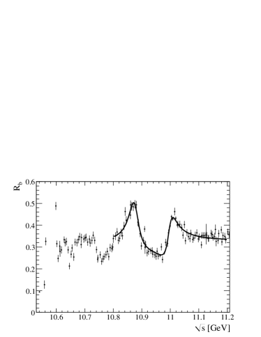
Figure 2: Measured $R_{b}$ as a function of $\sqrt{s}$ with the result of the fit with 2 Breit-Wigners described in :2008hx (left frame). Reprinted from Fig. 1 of B. Aubert et al. [BaBar Collaboration], Phys. Rev. Lett.  102, 012001 (2009) [Copyright (2009) by the American Physical Society]. The result of the fit with 4 Breit-Wigners described in the text is shown in the right-hand frame, where we have indicated the location of the $\Upsilon(5S)$, $\Upsilon(6S)$ and the tetraquark state $Y_{[b,q]}$ (labelled as $Y^{(1)}$). The location of the next higher $J^{PC}=1^{--}$ state $Y_{[b,q]}^{(2)}$ (labelled as $Y^{(2)}$) is also shown. The shaded bands around the mass of $Y^{(1)}$ and $Y^{(2)}$ reflect our theoretical uncertainty in the masses.

Table 9: Fit values of the masses, decay widths (both in MeV) and the strong phases $\phi$ (in radians).

	$M[MeV]$	$\Gamma[MeV]$	$\varphi$ [rad.]
$\Upsilon(5S)$	$10864\pm 5$	$46\pm 8$	$1.3\pm 0.3$
$\Upsilon(6S)$	$11007\pm 0.3$	$40\pm 2$	$0.88\pm 0.06$
$Y_{[b,l]}$	$10900-\Delta M/2\pm 2$	$28\pm 2$	$4.4\pm 0.2$
$Y_{[b,h]}$	$10900+\Delta M/2\pm 2$	$28\pm 2$	$1.9\pm 0.2$

In conclusion, we have presented a case for the observation of a hidden $b\bar{b}$ tetraquark states in the BaBar $R_{b}$-scan :2008hx . Our analysis is compatible with a $J^{PC}=1^{--}$ state $Y_{[bq]}(10900)$ having a width of about 30 MeV. A scan of $R_{b}$ in finer energy steps should be able to resolve the structure seen at this mass in terms of two mass eigenstates, split by about 6 MeV. The electronic widths are estimated to be between 50 and 120 electron volts. Other possible manifestations of tetraquarks have been discussed in the literature Hou:2006it ; Karliner:2008rc and a dynamical model for the decays $Y_{b}(10890)\to\Upsilon(1S,2S)\pi^{+}\pi^{-}$ is presented in Ali:2009es .

Acknowledgments

We thank the BaBar collaboration and the American Physical Society for their permission to show Fig. 2 (left frame) published in :2008hx . Helpful discussions with Riccardo Faccini and Antonello Polosa are gratefully acknowledged. We also thank Riccardo Faccini for providing us the fit program used in the BaBar analysis and we are grateful to Alexander Parkhomenko for reading the manuscript and pointing out several typos and notational inconsistencies in the first version of this paper. This work has been partially supported by funds provided by the ENSF, Trieste, Italy. Two of us (I.A. and M.J.A.) would like to thank DESY for the hospitality during the summer 2009, where this work was done. C.H. wants to thank Benjamin Lutz for discussion on some technical aspects of the fits.

References

(1)
B. Aubert et al. [BaBar Collaboration],
Phys. Rev. Lett. 102, 012001 (2009)
[arXiv:0809.4120 [hep-ex]],
and https://oraweb.slac.stanford.edu/pls/slacquery/babar-documents.startup
(2)
K. F. Chen et al. [Belle Collaboration],
Phys. Rev. Lett. 100, 112001 (2008)
[arXiv:0710.2577 [hep-ex]];
I. Adachi et al. [Belle Collaboration],
arXiv:0808.2445 [hep-ex].
(3)
C. Amsler et al. [Particle Data Group],
Phys. Lett. B 667, 1 (2008).
(4)
R. L. Jaffe,
Phys. Rept. 409, 1 (2005)
[Nucl. Phys. Proc. Suppl. 142, 343 (2005)]
[arXiv:hep-ph/0409065].
(5)
C. Quigg,
Nucl. Phys. Proc. Suppl. 142, 87 (2005)
[arXiv:hep-ph/0407124].
(6)
A. Zupanc [for the Belle Collaboration],
arXiv:0910.3404 [hep-ex].
(7)
B. Aubert et al. [BaBar Collaboration],
Phys. Rev. D 74, 091103 (2006)
[arXiv:hep-ex/0610018].
(8)
M. Ablikim et al. [BES Collaboration],
Phys. Rev. Lett. 100, 102003 (2008)
[arXiv:0712.1143 [hep-ex]].
(9)
C. P. Shen et al. [Belle Collaboration],
Phys. Rev. D 80, 031101 (2009)
[arXiv:0808.0006 [hep-ex]].
(10)
N. A. Tornqvist,
Phys. Lett. B 590, 209 (2004)
[arXiv:hep-ph/0402237].
E. Braaten and M. Kusunoki,
Phys. Rev. D 69, 074005 (2004)
[arXiv:hep-ph/0311147].
E. S. Swanson,
Phys. Lett. B 588, 189 (2004)
[arXiv:hep-ph/0311229].
M. B. Voloshin,
Phys. Lett. B 604, 69 (2004)
[arXiv:hep-ph/0408321].
C. E. Thomas and F. E. Close,
Phys. Rev. D 78, 034007 (2008)
[arXiv:0805.3653 [hep-ph]].
(11)
X. Liu, X. Q. Zeng and X. Q. Li,
Phys. Rev. D 72, 054023 (2005)
[arXiv:hep-ph/0507177].
X. Liu, Y. R. Liu, W. Z. Deng and S. L. Zhu,
Phys. Rev. D 77, 034003 (2008)
[arXiv:0711.0494 [hep-ph]].
X. Liu, Z. G. Luo, Y. R. Liu and S. L. Zhu,
Eur. Phys. J. C 61, 411 (2009)
[arXiv:0808.0073 [hep-ph]].
X. Liu and S. L. Zhu,
Phys. Rev. D 80, 017502 (2009)
[arXiv:0903.2529].
(12)
J. L. Rosner,
Phys. Rev. D 76, 114002 (2007)
[arXiv:0708.3496 [hep-ph]].
C. Meng and K. T. Chao,
arXiv:0708.4222 [hep-ph].
S. H. Lee, A. Mihara, F. S. Navarra and M. Nielsen,
Phys. Lett. B 661, 28 (2008)
[arXiv:0710.1029 [hep-ph]].
C. E. Thomas and F. E. Close,
Phys. Rev. D 78, 034007 (2008)
[arXiv:0805.3653 [hep-ph]].
N. Mahajan,
arXiv:0903.3107 [hep-ph].
T. Branz, T. Gutsche and V. E. Lyubovitskij,
Phys. Rev. D 80, 054019 (2009)
[arXiv:0903.5424 [hep-ph]].
(13)
E. Kou and O. Pene,
Phys. Lett. B 631, 164 (2005)
[arXiv:hep-ph/0507119].
F. E. Close and P. R. Page,
Phys. Lett. B 628, 215 (2005)
[arXiv:hep-ph/0507199].
(14)
L. Maiani, F. Piccinini, A. D. Polosa and V. Riquer,
Phys. Rev. D 71, 014028 (2005)
[arXiv:hep-ph/0412098].
(15)
L. Maiani, V. Riquer, F. Piccinini and A. D. Polosa,
Phys. Rev. D 72, 031502 (2005)
[arXiv:hep-ph/0507062].
L. Maiani, F. Piccinini, A. D. Polosa and V. Riquer,
AIP Conf. Proc. 814, 508 (2006)
[arXiv:hep-ph/0512082].
L. Maiani, A. D. Polosa and V. Riquer,
arXiv:0708.3997 [hep-ph].
L. Maiani, A. D. Polosa and V. Riquer,
New J. Phys. 10, 073004 (2008).
(16)
N. V. Drenska, R. Faccini and A. D. Polosa,
Phys. Lett. B 669, 160 (2008)
[arXiv:0807.0593 [hep-ph]].
N. V. Drenska, R. Faccini and A. D. Polosa,
Phys. Rev. D 79, 077502 (2009)
[arXiv:0902.2803 [hep-ph]].
(17)
S. K. Choi et al. [Belle Collaboration],
Phys. Rev. Lett. 91, 262001 (2003)
[arXiv:hep-ex/0309032].
(18)
D. E. Acosta et al. [CDF II Collaboration],
Phys. Rev. Lett. 93, 072001 (2004)
[arXiv:hep-ex/0312021].
(19)
V. M. Abazov et al. [D0 Collaboration],
Phys. Rev. Lett. 93, 162002 (2004)
[arXiv:hep-ex/0405004].
(20)
B. Aubert et al. [BaBar Collaboration],
Phys. Rev. D 71, 071103 (2005)
[arXiv:hep-ex/0406022].
(21)
C. Bignamini, B. Grinstein, F. Piccinini, A. D. Polosa and C. Sabelli,
Phys. Rev. Lett. 103, 162001 (2009)
[arXiv:0906.0882 [hep-ph]].
(22)
P. Artoisenet and E. Braaten,
arXiv:0911.2016 [hep-ph].
(23)
A. Abulencia et al. [CDF Collaboration],
Phys. Rev. Lett. 98, 132002 (2007)
[arXiv:hep-ex/0612053].
(24)
R. L. Jaffe,
Phys. Rev. D 15, 281 (1977).
R. L. Jaffe and F. E. Low,
Phys. Rev. D 19, 2105 (1979).
(25)
R. L. Jaffe and F. Wilczek,
Phys. Rev. Lett. 91, 232003 (2003)
[arXiv:hep-ph/0307341].
(26)
G. ’t Hooft, G. Isidori, L. Maiani, A. D. Polosa and V. Riquer,
Phys. Lett. B 662, 424 (2008)
[arXiv:0801.2288 [hep-ph]].
(27)
M. G. Alford and R. L. Jaffe,
Nucl. Phys. B 578, 367 (2000)
[arXiv:hep-lat/0001023];
N. Mathur et al.,
Phys. Rev. D 76, 114505 (2007)
[arXiv:hep-ph/0607110];
S. Prelovsek and D. Mohler,
Phys. Rev. D 79, 014503 (2009)
[arXiv:0810.1759 [hep-lat]];
H. Suganuma, K. Tsumura, N. Ishii and F. Okiharu,
Prog. Theor. Phys. Suppl. 168, 168 (2007)
[arXiv:0707.3309 [hep-lat]].
M. Loan, Z. H. Luo and Y. Y. Lam,
Eur. Phys. J. C 57, 579 (2008)
[arXiv:0907.3609 [hep-lat]];
S. Prelovsek, T. Draper, C. B. Lang, M. Limmer, K. F. Liu, N. Mathur and D. Mohler,
arXiv:0910.2749 [hep-lat].
(28)
C. Alexandrou, Ph. de Forcrand and B. Lucini,
Phys. Rev. Lett. 97, 222002 (2006)
[arXiv:hep-lat/0609004].
(29)
D. Ebert, R. N. Faustov and V. O. Galkin,
Mod. Phys. Lett. A 24, 567 (2009)
[arXiv:0812.3477 [hep-ph]].
(30)
Z. G. Wang,
arXiv:0908.1266 [hep-ph].
(31)
W. Buchmuller and S. H. H. Tye,
Phys. Rev. D 24, 132 (1981).
(32)
A. Ali, C. Hambrock and M. J. Aslam,
DESY Report 09-222 [arXiv:0912.5016 [hep-ph]].
(33)
A. De Rujula, H. Georgi and S. L. Glashow,
Phys. Rev. D 12, 147 (1975).
(34)
J. L. Domenech-Garret and M. A. Sanchis-Lozano,
Comput. Phys. Commun. 180, 768 (2009)
[arXiv:0805.2704 [hep-ph]].
(35)
We thank Riccardo Faccini for providing us the of the BaBar fit shown
in Fig. 1 of the BaBar paper :2008hx and the details of the modifications
in replacing the flat nonresonant term by a threshold function at .
(36)
W. S. Hou,
Phys. Rev. D 74, 017504 (2006)
[arXiv:hep-ph/0606016].
(37)
M. Karliner and H. J. Lipkin,
arXiv:0802.0649 [hep-ph].