On Bregman Distances and Divergences of Probability Measures

Abstract

The paper introduces scaled Bregman distances of probability distributions which admit non-uniform contributions of observed events. They are introduced in a general form covering not only the distances of discrete and continuous stochastic observations, but also the distances of random processes and signals. It is shown that the scaled Bregman distances extend not only the classical ones studied in the previous literature, but also the information divergence and the related wider class of convex divergences of probability measures. An information processing theorem is established too, but only in the sense of invariance w.r.t. statistically sufficient transformations and not in the sense of universal monotonicity. Pathological situations where coding can increase the classical Bregman distance are illustrated by a concrete example. In addition to the classical areas of application of the Bregman distances and convex divergences such as recognition, classification, learning and evaluation of proximity of various features and signals, the paper mentions a new application in 3D-exploratory data analysis. Explicit expressions for the scaled Bregman distances are obtained in general exponential families, with concrete applications in the binomial, Poisson and Rayleigh families, and in the families of exponential processes such as the Poisson and diffusion processes including the classical examples of the Wiener process and geometric Brownian motion.

Index Terms — Bregman distances, classification, divergences, exponential distributions, exponential processes, information retrieval, machine learning, statistical decision, sufficiency.

I Introduction

Bregman (1967) introduced for convex functions $\phi:\mathbb{R}^{d}\rightarrow\mathbb{R}$ with gradient $\triangledown\phi$ the $\phi$-depending nonnegative measure of dissimilarity

$$B_{\phi}(p,q)=\phi(p)-\phi(q)-\triangledown\phi(q)(p-q)$$ (1)

of $d$-dimensional vectors $p,q\in\mathbb{R}^{d}$. His motivation was the problem of convex programming, but in the subsequent literature it became widely applied in many other problems under the name Bregman distance in spite of that it is not in general the usual metric distance (it is a pseudodistance which is reflexive but neither symmetric nor satisfying the triangle inequality). The most important feature is the special separable form defined by

$$B_{\phi}(p,q)=\sum_{i=1}^{d}\left[\phi(p_{i})-\phi(q_{i})-\phi^{\prime}(q_{i})(p_{i}-q_{i})\right]$$ (2)

for vectors $p=(p_{1},...,p_{d}),q=(q_{1},...,q_{d})$ and convex differentiable functions $\phi:\mathbb{R}\rightarrow\mathbb{R}$. For example, the function $\phi(t)=(t-1)^{2}$ leads to the classical squared Euclidean distance

$$B_{\phi}(p,q)=\sum_{i=1}^{d}\left(p_{i}-q_{i}\right)^{2}.$$ (3)

In the optimization-theoretic context the Bregman distances are usually studied in the general form (1) – see, e.g., Csiszár and Matúš (2008, 2009), as well as Bauschke and Borwein (1997) for adjecent random projection studies. In the information-theoretic or statistical context they are typically used in the separable form (2) for vectors $p,q$ with nonnegative coordinates representing generalized distributions (finite discrete measures) and functions $\phi:[0,\infty)\rightarrow\mathbb{R}$ differentiable on $(0,\infty)$ (the problem with $q_{i}=0$ is solved by resorting to the right-hand derivative $\phi_{+}^{\prime}(0)$). The concrete example $\phi(t)=t\ln t$ leads to the well-known Kullback divergence

$$B_{\phi}(p,q)=\sum_{i=1}^{d}p_{i}\ln\frac{p_{i}}{q_{i}}.$$

Of course, the most common context are discrete probability distributions $p,q$ since vectors of hypothetical or observed frequencies $p,q$ are easily transformed to the relative frequencies normed to $1$. For example, Csiszár (1991, 1994, 1995) or Pardo and Vajda (1997, 2003) used the Bregman distances of probability distributions in the context of information theory and asymptotic statistics.

Important alternatives to the Bregman distances (2) are the $\phi$- divergences defined by

$$D_{\phi}(p,q)=\sum_{i=1}^{d}q_{i}\phi\left(\frac{p_{i}}{q_{i}}\right)$$ (4)

for functions $\phi$ which are convex on $[0,\infty)$, continuous on $(0,\infty)$ and strictly convex at $1$ with $\phi(1)=0$. Originating in the paper of Csiszár (1963), they share some properties with the Bregman distances (2), e.g., they are pseudodistances too. For example, the above considered functions $\phi(t)=(t-1)^{2}$ and $\phi(t)=t\ln t$ lead in this case to the classical Pearson divergence

$$D_{\phi}(p,q)=\sum_{i=1}^{d}\frac{\left(p_{i}-q_{i}\right)^{2}}{q_{i}}$$ (5)

and the above mentioned Kullback divergence $D_{\phi}(p,q)\equiv B_{\phi}(p,q)$ which are asymmetric in $p,q$ and contradict the triangle inequality. On the other hand, $\phi(t)=|t-1|$ leads to the L₁-norm $||p-q||$ which is a metric distance and $\phi(t)=(t-1)^{2}/(t+1)$ defines the LeCam divergence

$$D_{\phi}(p,q)=\sum_{i=1}^{d}\frac{\left(p_{i}-q_{i}\right)^{2}}{p_{i}+q_{i}}$$

which is a squared metric distance (for more about the metricity of $\phi$ -divergences the reader is referred to Vajda (2009)).

However, there exist also some sharp differences between these two types of pseudodistances of distributions. One distinguising property of Bregman distances is that their use as loss criterion induces the conditional expectation as outcoming unique optimal predictor from given data (cf. Banerjee at al. (2005a)); this is for instance used in Banerjee et al. (2005b) for designing generalizations of the $k$-means algorithm which deals with the special case of squared Euclidean error (3) (cf. the seminal work of Lloyd (1982) reprinting a Technical Report of Bell Laboratories dated by 1957). These features are generally not shared by those of the $\phi$-divergences which are not Bregman distances, e.g., by the Pearson divergence (5). On the other hand, a distinguishing property of $\phi$-divergences is the information processing property, i.e., the impossibility to increase the value $D_{\phi}(p,q)$ by transformations of the observations distributed by p, q and preservation of this value by the statistically sufficient transformations (Csiszár (1967), see in this respect also Liese and Vajda (2006)). This property is not shared by the Bregman distances which are not $\phi$-divergences. For example, the distributions $p=(1/2,1/4,1/4)$ and $q=(1,0,0)$ are mutually closer (less discernible) in the Euclidean sense (3) than their reductions $\tilde{p}=(1/2,1/2)$ and $\tilde{q}=(1,0)$ obtained by merging the second and third observation outcomes into one.

Depending on the need to exploit one or the other of these distinguished properties, the Bregman distances or Csiszár divergences are preferred, and both of them are widely applied in important areas of information theory, statistics and computer science, for example in

(Ai)   information retrieval (see, e.g., Do and Vetterli (2002), Hertz at al. (2004)),

(Aii)  optimal decision (for general decision see, e.g., Boratynska (1997), Freund et al. (1997), Bartlett et al. (2006), Vajda and Zvárová (2007), for speech processing see, e.g., Carlson and Clements (1991), Veldhuis and Klabers (2002), for image processing see, e.g., Xu and Osher (2007), Marquina and Osher (2008), Scherzer et al. (2008)), and

(Aiii) machine learning (see, e.g., Laferty (1999), Banerjee et al. (2005), Amari (2007), Teboulle (2007), Nock and Nielsen (2009)).

(Aiv) parallel optimization and computing (see, e.g., Censor and Zenios (1997)).

In this context it is obvious the importance of the functionals of distributions which are simultaneously divergences in both the Csiszár and Bregman sense or, more broadly, of the research of relations between the Csiszár and Bregman divergences. This paper is devoted to this research. It generalizes the separable Bregman distances (2) as well as the $\phi$-divergences (4) by introducing the scaled Bregman distances which for the discrete setup reduce to

$$B_{\phi}(p,q|m) = \sum_{i=1}^{d}\Big{[}\phi(p_{i}/m_{i})-\phi(q_{i}/m_{i})$$ (6)

$$-\phi_{+}^{\prime}(q_{i}/m_{i})(p_{i}/m_{i}-q_{i}/m_{i})\Big{]}m_{i}$$

for arbitrary finite scale vectors $m=(m_{1},...,m_{d}),$ convex functions $\phi$ and right-hand derivatives $\phi_{+}^{\prime}$. Obviously, the uniform scales $m=(1,...,1)$ lead to the Bregman distances (2) and the probability distribution scales $m=$ $q$ $=(q_{1},...,q_{d})$ lead to the $\phi$-divergences (4). We shall work out further interesting relations of the $B_{\phi}(p,q|m)$ distances to the $\phi$-divergences $D_{\phi}(p,q)$ and $D_{\phi}(p,m)\$ and evaluate explicit formulas for the stochastically scaled Bregman distances in arbitrary exponential families of distributions, including also the non-discrete setup.

Section II defines the $\phi$-divergences $D_{\phi}(P,M)$ of general probability measures $P$ and arbitrary finite measures $M$ and briefly reviews their basic properties. Section III introduces scaled Bregman distances $B_{\phi}(P,Q|M)$ and investigates their relations to the $\phi$ -divergences $D_{\phi}(P,Q)$ and $D_{\phi}(P,M).$ Section IV studies in detail the situation where all three measures $P,Q,M$ are from the family of general exponential distributions. Finally, Section V illustrates the results by investigating concrete examples of $P,Q,M$ from classical statistical families as well as from a family of important random processes.

Notational conventions

Throughout the paper, $\mathfrak{M}$ denotes the space of all finite measures on a measurable space $({\mathcal{X}},{\mathcal{A}})$ and $\mathfrak{P}\subset\mathfrak{M}$ the subspace of all probability measures. Unless otherwise explicitly stated $P,Q,M\,$are mutually measure-theoretically equivalent measures on $({\mathcal{X}},{\mathcal{A}})$ dominated by a $\sigma$-finite measure $\lambda$ on $({\mathcal{X}},{\mathcal{A}})$. Then the densities

$$p={\frac{\mathrm{d}P}{\mathrm{d}\lambda}},\quad q={\frac{\mathrm{d}Q}{\mathrm{d}\lambda}}\qquad\mbox{and}\qquad m={\frac{\mathrm{d}M}{\mathrm{d}\lambda}}$$ (7)

have a common support which will be identified with $\mathcal{X}$ (i.e., the densities (7) are positive on $\mathcal{X}$). Unless otherwise explicitly stated, it is assumed that $P,Q\in\mathfrak{P}$,   $M\in\mathfrak{M}$ and that $\phi:(0,\infty)\mapsto{\mathbb{R}}$ is a continuous and convex function. It is known that then the possibly infinite extension $\phi(0)=\lim_{t\downarrow 0}\phi(t)$ and the right-hand derivatives $\phi_{+}^{\prime}(t)$ for $t\in[0,\infty)$ exist, and that the adjoint function

$$\phi^{\ast}(t)=t\phi(1/t)$$ (8)

is continuous and convex on $(0,\infty)$ with possibly infinite extension $\phi^{\ast}(0)$. We shall assume that $\ \phi(1)\equiv\phi^{\ast}(1)=0.$

II DIVERGENCES

For $P\,\in\mathfrak{P}$ and $M\in\mathfrak{M}$ we consider

$$D_{\phi}(P,M)=\int_{{\mathcal{X}}}\phi\left({\frac{p}{m}}\right)\mathrm{d}M=\int_{{\mathcal{X}}}m\,\phi\left({\frac{p}{m}}\right)\mathrm{d}\lambda\qquad(cf.\ (\ref{d}))$$ (9)

generated by the same convex functions as considered in the formula (4) for discrete $P$ and $M$. An important special case is $D_{\phi}(P,Q)$ with $Q\in\mathfrak{P}$.

The existence (but possible infinity) of the $\phi$-divergences follows from the bounds

$$\phi_{+}^{\prime}(1)(p-m)\ \leq\ m\,\phi\left({\frac{p}{m}}\right)\ \leq\ m\,\phi(0)+p\,\phi^{\ast}(0)$$ (10)

on the integrand, leading to the $\phi$-divergence bounds

$$\phi_{+}^{\prime}(1)(1-M(\mathcal{X}))\ \leq\ D_{\phi}(P,M)\ \leq\ M(\mathcal{X})\,\phi(0)+\phi^{\ast}(0).$$ (11)

The integrand bounds (10) follow by putting $s=1$ and $t=p/m$  in the inequality

$$\phi(s)+\phi_{+}^{\prime}(s)(t-s)\leq\phi(t)\leq\phi(0)+t\phi^{\ast}(0),$$ (12)

where the left-hand side is the well-known support line of $\phi(t)$ at $t=s.$ The right-hand inequality is obvious for $\phi(0)=\infty$. If $\phi(0)<\infty$ then it follows by taking $s\rightarrow\infty$ in the inequality

$$\phi(t)\leq\phi(0)\,+\,t\ \frac{\phi(s)-\phi(0)}{s}\ ,$$

obtained from the Jensen inequality for $\phi(t)$ situated between $\phi(0)$ and $\phi(s)$. Since the function $\psi(p,m)=m\phi(p/m)$ is homogeneous of order 1 in the sense $\psi(tp,tm)=t\psi(p,m)$ for all $t>0,$ the divergences (9) do not depend on the choice of the dominating measure $\lambda$.

Notice that $D_{\phi}(P,M)$ might be negative. For probability measures $P,Q$ the bounds (11) take on the form

$$0\leq D_{\phi}(P,Q)\leq\phi(0)+\phi^{\ast}(0),\vskip 6.0pt plus 2.0pt minus 2.0pt$$ (13)

and the equalities are achieved under well-known conditions (cf. Liese and Vajda (1987), (2006)): the left equality holds if $P=Q$, and the right one holds if $P\perp Q$ (singularity). Moreover, if $\phi(t)$ is strictly convex at $t=1,$ the first if can be replaced by iff,  and in the case $\phi(0)+\phi^{\ast}(0)<\infty$ also the second if can be replaced by iff.

An alternative to the left-hand inequality in (11), which extends the left-hand inequality in (13) including the conditions for the equality, is given by the following statement (for a systematic theory of $\phi$-divergences of finite measures we refer to the recent paper of Stummer and Vajda (2010)).

Lemma 1

For every $P\in\mathfrak{P}$, $M\in\mathfrak{M}$ one gets the lower divergence bound

$$M({\mathcal{X}})\,\phi\left({\frac{1}{M({\mathcal{X}})}}\right)\leq D_{\phi}(P,M)\ ,$$ (14)

where the equality holds if

$$p\ =\ {\frac{m}{M({\mathcal{X}})}}\text{ \ \ \ \ }P\text{-a.s.}$$ (15)

If $D_{\phi}(P,M)<\infty$ and $\phi(t)$ is strictly convex at $t=1/M({\mathcal{X}}),$ the equality in (14) holds if and only if (15 ) holds.

Proof

By (9) and the definition (8) of the convex function $\phi^{\ast}$

$$D_{\phi}(P,M)=\int_{{\mathcal{X}}}\phi^{\ast}\left({\frac{m}{p}}\right)\mathrm{d}P.$$

Hence by Jensen’s inequality

$$D_{\phi}(P,M)\geq\phi^{\ast}\left(\int_{{\mathcal{X}}}{\frac{m}{p}}\,\mathrm{d}P\right)=\phi^{\ast}(M({\mathcal{X}}))$$ (16)

which proves the desired inequality (14). Since

$${\frac{m}{p}}\ =\ M({\mathcal{X}})\quad P\mbox{-a.\,s.}$$

is the condition for equality in (16), the rest is clear from the easily verifiable fact that $\phi^{\ast}(t)$ is strictly convex at $t=s$ if and only if $\phi(t)$ is strictly convex at $t=1/s$. $\square$

For some of the representation investigations below, it will also be useful to take into account that for probability measures $P,Q$ we get directly from definition (9) the “skew symmetry” $\phi$-divergence formula

$$D_{\phi^{\ast}}(P,Q)=D_{\phi}(Q,P)\ ,$$

as well as the sufficiency of the condition

$$\phi(t)-\phi^{\ast}(t)\ \equiv\ \text{constant}\,\mathbf{\cdot}\,(t-1)$$ (17)

for the $\phi$-divergence symmetry

$$D_{\phi}(P,Q)=D_{\phi}(Q,P)\mbox{ \ \ for all }P,Q\mbox{\ }.$$ (18)

Liese and Vajda (1987) proved that under the assumed strict convexity of $\phi(t)$ at $t=1$ the condition (17) is is not only sufficient but also necessary for the symmetry (18).

III SCALED BREGMAN DISTANCES

Let us now introduce the basic concept of the current paper, which is a measure-theoretic version of the Bregman distance (6). In this definition it is assumed that $\phi$ is a finite convex function in the domain $t>0,$ continuously extended to $t=0$. As before, $\phi_{+}^{\prime}(t)$ denotes the right-hand derivative which for such $\phi(t)$ exists and $p,q,m$ are the densities defined in (7).

Definition 1

The Bregman distance of probability measures $P,\,Q$ scaled by an arbitrary measure $M$ on $(\mathcal{X},\mathcal{A})$ measure-theoretically equivalent with $P,\,Q$ is defined by the formula

$$B_{\phi}\left(P,Q\,|\,M\right)$$

$$=\int_{{\mathcal{X}}}\left[\phi\left({\frac{p}{m}}\right)-\phi\left({\frac{q}{m}}\right)-\phi_{+}^{\prime}\left({\frac{q}{m}}\right)\left(\frac{p}{m}-\frac{q}{m}\right)\right]\mathrm{d}M$$

(19)

$$=\int_{{\mathcal{X}}}\left[m\phi\left({\frac{p}{m}}\right)-m\phi\left({\frac{q}{m}}\right)-\phi_{+}^{\prime}\left({\frac{q}{m}}\right)(p-q)\right]\mathrm{d}\lambda.$$

The convex $\phi$ under consideration can be interpreted as a generating function of the distance.

Remarks 1

(1) By putting $t=p/m$ and $s=q/m$ in (12) we find the argument of the integral in (19) to be nonnegative. Hence the Bregman distance $B_{\phi}\left(P,Q\,|\,M\right)$ is well-defined by (19) and is always nonnegative (possibly infinite).
(2) Notice that the integrand in the first (respectively second) integral of (19) constitutes a function, say, $\widetilde{\Upsilon}(p,q,m)$ (respectively $\Upsilon(p,q,m)$) which is homogeneous of order $0$ (respectively order $1$), i.e., for all $t>0$ there holds $\widetilde{\Upsilon}(tp,tq,tm)=\widetilde{\Upsilon}(p,q,m)$ (respectively $\Upsilon(tp,tq,tm)=t\cdot\Upsilon(p,q,m)$). Analogously, as already partially indicated above, the integrand in the first (respectively second) integral of (9) is also a function, say, $\widetilde{\psi}(p,m)$ (respectively $\psi(p,m)$) which is homogeneous of order $0$ (respectively order $1$).
(3) In our measure-theoretic context (19) we have incorporated the possible non-differentiability of $\phi$ by using its right-hand derivative, which will be essential at several places below. For general Banach spaces, one typically employs various directional derivatives – see, e.g., Butnariu and Resmerita (2006) in connection with different types of convexity properties.

The special scaled Bregman distances $B_{\phi}\left(P,Q\,|\,M\right)$ for probability scales $M\in\mathfrak{P}$ were introduced by Stummer (2007). Let us mention some other important previously considered special cases.

(a) For $\mathcal{X}$ finite or countable and counting measure $M=\lambda$ some authors were already cited above in connection with the formula (2) and the research areas (Ai) - (Aiii). In addition to them, one can mention also Byrne (1999), Collins et al. (2002), Murata et al. (2004), Cesa-Bianchi and Lugosi (2006).

(b) For open Euclidean set $\mathcal{X}$ and Lebesgue measure $M=\lambda$ on it one can mention Jones and Byrne (1990), as well as Resmerita and Anderssen (2007).

In the rest of this paper, we restrict ourselves to the Bregman distances $B_{\phi}\left(P,Q\,|\,M\right)$ scaled by finite measures $M\in\mathcal{M}$ and to the same class of convex functions as considered in the $\phi$-divergence formulas (4) and (9). By using the remark after Definition 1 and applying (12) we get

$$D_{\phi}(P,M)\geq D_{\phi}(Q,M)+\int_{\mathcal{X}}\phi_{+}^{\prime}\left({\frac{q}{m}}\right)(p-q)\mathrm{d}\lambda$$

if at least one of the right-hand side expressions is finite. Similarly,

$$B_{\phi}\left(P,Q\,|\,M\right)=D_{\phi}(P,M)-D_{\phi}(Q,M)-\int_{\mathcal{X}}\phi_{+}^{\prime}\left({\frac{q}{m}}\right)\mathrm{d}\lambda$$ (20)

if at least two of the right-hand side expressions are finite (which can be checked, e.g., by using (11) or (14)).

The formula (19) simplifies in the important special cases $M=P$ and $M=Q$. In the first case, due to $\phi(1)=0$ it reduces to

$$B_{\phi}\left(P,Q\,|\,P\right)=\int_{{\mathcal{X}}}\left[\phi_{+}^{\prime}\left({\frac{q}{p}}\right)(q-p)-p\phi\left({\frac{q}{p}}\right)\right]\mathrm{d}\lambda\vskip 6.0pt plus 2.0pt minus 2.0pt$$

$$=\ \int_{{\mathcal{X}}}\phi_{+}^{\prime}\left({\frac{q}{p}}\right)(q-p)\mathrm{d}\lambda-D_{\phi}(Q,P)\ ,$$ (21)

where the difference (21) is meaningful if and only if $D_{\phi}(Q,P)\equiv D_{\phi^{\ast}}(P,Q)$ is finite. The nonnegative divergence measure $\mathcal{B}_{\phi}\left(P,Q\right):=B_{\phi}\left(P,Q\,|\,P\right)$ is thus the difference between the nonnegative dissimilarity measure

$$\mathcal{D}_{\phi}\left(Q,P\right)=\int_{{\mathcal{X}}}\phi_{+}^{\prime}\left({\frac{q}{p}}\right)(q-p)\,\mathrm{d}\lambda\ \geq\ D_{\phi}(Q,P)$$

and the nonnegative $\phi-$divergence $D_{\phi}(Q,P)$. Furthermore, in the second special case $M=Q$ the formula (19) leads to the equality

$$B_{\phi}\left(P,Q\,|\,Q\right)=D_{\phi}(P,Q)$$ (22)

without any restriction on $P,Q\in\mathfrak{P}$ as realized already by Stummer (2007).

Conclusion 1

Equality (22) – together with the fact that $B_{\phi}\left(P,Q\,|\,M\right)$ depends in general on $M$ (see, e.g., Subsection B below) – shows that the concept of scaled Bregman distance (19) strictly generalizes the concept of $\phi-$divergence $D_{\phi}(P,Q)$ of probability measures $P,Q$.

Example 1

As an illustration not considered earlier we can take the non-differentiable function $\phi(t)=|t-1|$ for which

$$B_{\phi}\left(P,Q\,|\,Q\right)=V(P,Q)$$

i.e., this particular scaled Bregman distance reduces to the well known total variation.

As demonstrated by an example in the Introduction, measurable transformations (statistics)

$$T:(\mathcal{X},\mathcal{A})\mapsto(\mathcal{Y},\mathcal{B})$$ (23)

which are not sufficient for the pair $\{P,Q\}$ can increase those of the scaled Bregman distances $B_{\phi}\left(P,Q\,|\,M\right)$ which are not $\phi$ -divergences. On the other hand, the transformations (23) which are sufficient for the pair $\{P,Q\}$ need not preserve these distances either. Next we formulate conditions under which the scaled Bregman distances $B_{\phi}\left(P,Q\,|\,M\right)$ are preserved by transformations of observations.

Definition 2

We say that the transformation (23) is sufficient for the triplet $\{P,\,Q,\,M\}$ if there exist measurable functions $g_{P},g_{Q},g_{M}:\mathcal{Y}\mapsto\mathbb{R}$ and $h:\mathcal{X}\mapsto\mathbb{R}$ such that

$$p(x)=g_{P}(Tx)h(x),\text{ \ }q(x)=g_{Q}(Tx)h(x)$$

$$\text{and \ }m(x)=g_{M}(Tx)h(x).$$ (24)

If $M$ is probability measure then our definition reduces to the classical statistical sufficiency of the statistic $T$ for the family $\{P,\,Q,\,M\}$ (see pp. 18-19 in Lehman (2005)). All transformations (23) induce the probability measures $PT^{-1}$, $QT^{-1}$ and the finite measure $MT^{-1}$ on $(\mathcal{Y},\mathcal{B})$. We prove that the scaled Bregman distances of induced probability measures $PT^{-1}$, $QT^{-1}$ scaled by $MT^{-1}$ are preserved by sufficient transformations $T$.

Theorem 1

The transformations (23) sufficient for the triplet $\{P,Q,\,M\}$ preserve the scaled Bregman distances in the sense that

$$B_{\phi}\left(PT^{-1},QT^{-1}\,|\,MT^{-1}\right)=B_{\phi}\left(P,Q\,|\,M\right).$$ (25)

Proof.

By (19) and (24), the right-hand side of (25) is equal to

$$\int_{\mathcal{X}}\left[\phi_{P,M}\left(Tx\right)-\phi_{Q,M}\left(Tx\right)-\Delta_{P,Q,M}\left(Tx\right)\right]\mathrm{d}M$$ (26)

for

$$\phi_{P,M}\left(y\right)=\phi\left(\frac{g_{P}(y)}{g_{M}(y)}\right),\text{ \ }\phi_{Q,M}\left(y\right)=\phi\left(\frac{g_{Q}(y)}{g_{M}(y)}\right)$$ (27)

and

$$\Delta_{P,Q,M}\left(y\right)=\phi_{+}^{{}^{\prime}}\left(\frac{g_{Q}(y)}{g_{M}(y)}\right)\left(g_{P}(y)-g_{Q}(y)\right).$$ (28)

By Theorem D in Section 39 of Halmos (1964), the integral (26) is equal to

$$\int_{\mathcal{Y}}\left[\phi_{P,M}\left(y\right)-\phi_{Q,M}\left(y\right)-\Delta_{P,Q,M}\left(y\right)\right]\mathrm{d}MT^{-1}$$ (29)

and, moreover,

$$P(T^{-1}B)=\int_{B}g_{P}(y)\,h(T^{-1}y)\,\mathrm{d}\lambda T^{-1}$$

and similarly for $Q$ instead of $P$. Therefore

$$\frac{\mathrm{d}PT^{-1}}{\mathrm{d}\lambda T^{-1}}=g_{P}(y)\,h(T^{-1}y)\text{ \ and \ }\frac{\mathrm{d}QT^{-1}}{\mathrm{d}\lambda T^{-1}}=g_{Q}(y)\,h(T^{-1}y)$$

which together with (27), (28) and (19) implies that the integral (29) is nothing but the left-hand side of (25). This completes the proof. $\square$

Remark 2

Notice that by means of Remark 1(2) after Definition 1, the assertion of Theorem 1 can be principally related to the preservation of $\phi-$divergences by transformations which are sufficient for the pair $\{P,Q\}$ .

In the rest of this section we discuss some important special classes of scaled Bregman distances obtained for special distance-generating functions $\phi$.

III-A Bregman logarithmic distance

Let us consider the special function $\phi(t)=t\ln t$. Then $\phi^{\prime}(t)=\ln t+1$ so that (19) implies

$$B_{t\ln t}\left(P,Q\,|\,M\right)$$

$$=\int_{{\mathcal{X}}}\left[p\ln{\frac{p}{m}}-q\ln{\frac{q}{m}}-\left(\ln{\frac{q}{m}}+1\right)(p-q)\right]\mathrm{d}\lambda$$

$$=\int_{{\mathcal{X}}}\left[p\ln{\frac{p}{m}}-p\ln{\frac{q}{m}}\right]\mathrm{d}\lambda$$

$$=\ \int_{{\mathcal{X}}}p\ln{\frac{p}{q}}\,\mathrm{d}\lambda\ =\ D_{t\ln t}\left(P,Q\right)\ .$$ (30)

Thus, for $\phi(t)=t\ln t$ the Bregman distance $B_{\phi}\left(P,Q\,|\,M\right)$ exceptionally does not depend on the choice of the scaling and reference measures $M$ and $\lambda$; in fact, it always leads to the Kulllback-Leibler information divergence (relative entropy) $D_{t\ln t}(P,Q)$ (cf. Stummer (2007)). As a side effect, this independence gives also rise to examples for the conclusion that the validity of (25) does generally not imply that $T$ is sufficient for the triplet $\{P,\,Q,\,M\}$.

III-B Bregman reversed logarithmic distance

Let now $\phi(t)=-\ln t$ so that $\phi^{\prime}(t)=-1/t$. Then (19) implies

$$B_{-\ln t}\left(P,Q\,|\,M\right)$$

$$=\int_{{\mathcal{X}}}\left[m\ln{\frac{m}{p}}-m\ln{\frac{m}{q}}+{\frac{m}{q}}(p-q)\right]\mathrm{d}\lambda\vskip 6.0pt plus 2.0pt minus 2.0pt$$ (31)

$$=D_{t\ln t}(M,P)-D_{t\ln t}(M,Q)+\int_{{\mathcal{X}}}{\frac{mp}{q}}\,\mathrm{d}\lambda-M({\mathcal{X}})\vskip 6.0pt plus 2.0pt minus 2.0pt$$ (32)

$$=D_{-\ln t}(P,M)-D_{-\ln t}(Q,M)+\int_{{\mathcal{X}}}{\frac{mp}{q}}\mathrm{d}\lambda-M({\mathcal{X}})$$ (33)

where the equalities (32) and (33) hold if at least two out of the first three expressions on the right-hand side are finite. In particular, (31) implies (consistent with (22))

$$B_{-\ln t}\left(P,Q\,|\,Q\right)=D_{-\ln t}(P,Q)\quad$$ (34)

and (32) implies for $D_{t\ln t}(P,Q)<\infty$ (consistent with (21))

$$B_{-\ln t}\left(P,Q\,|\,P\right)=\chi^{2}(P,Q)-D_{t\ln t}(P,Q)\$$ (35)

where

$$\chi^{2}(P,Q)=\int_{{\mathcal{X}}}{\frac{(p-q)^{2}}{q}}\,\mathrm{d}\lambda$$

is the well-known Pearson information divergence. From (34) and (35) one can also see that the Bregman distance $B_{\phi}\left(P,Q\,|\,M\right)$ does in general depend on the choice of the reference measure $M$.

III-C Bregman power distances

In this subsection we restrict ourselves for simplicity to probability measures $M\in\mathfrak{P}$, i.e., we suppose $M(\mathcal{X})=1$. Under this assumption we investigate the scaled Bregman distances

$$B_{\alpha}\left(P,Q\,|\,M\right)=B_{\phi_{\alpha}}\left(P,Q\,|\,M\right)\ ,\quad\alpha\in\mathbb{R},\ \alpha\neq 0,\ \alpha\neq 1$$ (36)

for the family of power convex functions

$$\phi(t)\equiv\phi_{\alpha}(t)={\frac{t^{\alpha}-1}{\alpha(\alpha-1)}}\mbox{ \ \ with \ }\phi_{\alpha}^{\prime}(t)={\frac{t^{\alpha-1}}{\alpha-1}\ .}$$ (37)

For comparison and representation purposes, we use for $P$ (and analogously for $Q$ instead of $P$) the power divergences

$$D_{\alpha}(P,M)=D_{\phi_{\alpha}}(P,M)$$

$$=\frac{1}{\alpha(\alpha-1)}\left[\int_{{\mathcal{X}}}p^{\alpha}\,m^{1-\alpha}\,\mathrm{d}\lambda-1\right]\vskip 12.0pt plus 4.0pt minus 4.0pt$$

$$=\frac{\exp\rho_{\alpha}(P,M)-1}{\alpha(\alpha-1)}\ \text{\ \ with }\rho_{\alpha}(P,M)=\ln\int_{{\mathcal{X}}}p^{\alpha}\,m^{1-\alpha}\,\mathrm{d}\lambda$$

(38)

of real powers $\alpha$ different from $0$ and $1$, studied for arbitrary probability measures $P,M$ in Liese and Vajda (1987). They are one-one related to the Rényi divergences

$$R_{\alpha}(P,M)=\frac{\rho_{\alpha}(P,M)}{\alpha(\alpha-1)},\mbox{ \ \ }\alpha\in\mathbb{R},\mbox{ }\alpha\neq 0,\mbox{ }\alpha\neq 1,$$

introduced in Liese and Vajda (1987) as an extension of the original narrower class of the divergences

$$R_{\alpha}(P,M)=\frac{\rho_{\alpha}(P,M)}{\alpha-1},\mbox{ \ \ }\alpha>0,\mbox{ }\alpha\neq 1$$

of Rényi (1961).

Returning now to the Bregman power distances, observe that if $D_{\alpha}(P,M)+D_{\alpha}(Q,M)\$is finite then (20), (36) and (37) imply for $\alpha\neq 0,\ \alpha\neq 1$

$$B_{\alpha}(P,Q\,|\,M)$$

$$=-D_{\alpha}(Q,M)-{\frac{1}{\alpha-1}}\int_{{\mathcal{X}}}\left({\frac{q}{m}}\right)^{\alpha-1}(p-q)\,\mathrm{d}\lambda\vskip 6.0pt plus 2.0pt minus 2.0pt$$

$$=D_{\alpha}(P,M)-D_{\alpha}(Q,M)$$

$$\hskip 19.91684pt-{\frac{1}{\alpha-1}}\int_{{\mathcal{X}}}\left[\left({\frac{q}{m}}\right)^{\alpha-1}\!\!\!p-\left({\frac{q}{m}}\right)^{\alpha}m\right]\mathrm{d}\lambda\vskip 6.0pt plus 2.0pt minus 2.0pt$$

$$=D_{\alpha}(P,M)-(1\!-\!\alpha)\,D_{\alpha}(Q,M)$$

$$\hskip 19.91684pt-{\frac{1}{\alpha\!-\!1}}\left[\int_{{\mathcal{X}}}\left(\frac{q}{m}\right)^{\alpha-1}\!\!\!p\,\mathrm{d}\lambda-1\right].$$ (39)

In particular, we get from here (consistent with (22))

$$B_{\alpha}(P,Q\,|\,Q)=D_{\alpha}(P,Q)\quad$$

and in case of $D_{\alpha}(Q,P)\equiv D_{1-\alpha}(P,Q)<\infty$ also

$$B_{\alpha}(P,Q\,|\,P)=(\alpha-2)\,D_{\alpha-1}(Q,P)+(\alpha-1)\,D_{\alpha}(Q,P)$$

$$\equiv(\alpha-2)\,D_{2-\alpha}(P,Q)+(\alpha-1)\,D_{1-\alpha}(P,Q).$$

In the following theorem, and elsewhere in the sequel, we use the simplified notation

$$D_{1}(P,M)=D_{t\ln t}(P,M)\mbox{ \ and \ }D_{0}(P,M)=D_{-\ln t}(P,M)$$

for the probability measures $P,M$ under consideration (and also later on where $M$ is only a finite measure). This step is motivated by the limit relations

$$\lim_{\alpha\downarrow 0}D_{\alpha}(P,M) = D_{-\ln t}(P,M)\mbox{ \quad and \ }$$

$$\lim_{\alpha\uparrow 1}D_{\alpha}(P,M) = D_{t\ln t}(P,M)$$ (40)

proved as Proposition 2.9 in Liese and Vajda (1987) for arbitrary probability measures $P,M$. Applying these relations to the Bregman distances, we obtain

Theorem 2

If $D_{0}(P,M)+D_{0}(Q,M)<\infty$ then

$$\lim_{\alpha\downarrow 0}B_{\alpha}(P,Q\,|\,M)$$

$$=D_{0}(P,M)-D_{0}(Q,M)+\int_{{\mathcal{X}}}{\frac{mp}{q}}\,\mathrm{d}\lambda-1$$ (41)

$$=B_{-\ln t}(P,Q\,|\,M).$$ (42)

If $D_{1}(P,M)+D_{1}(Q,M)<\infty$ and

$$\lim_{\beta\downarrow 0}\int_{{\mathcal{X}}}{\frac{(q/m)^{-\beta}-1}{\beta}}\,\mathrm{d}P$$

$$=\int_{{\mathcal{X}}}\lim_{\beta\downarrow 0}{\frac{(q/m)^{-\beta}-1}{\beta}}\,\mathrm{d}P=-\int_{{\mathcal{X}}}\ln{\frac{q}{m}}\,\mathrm{d}P$$ (43)

then

$$\lim_{\alpha\uparrow 1}B_{\alpha}(P,Q\,|\,M)=D_{1}(P,M)-\int_{{\mathcal{X}}}\ln{\frac{q}{m}}\,\mathrm{d}P$$ (44)

$$=D_{1}(P,Q)\ =\ B_{t\ln t}(P,Q\,|\,M)\ .$$ (45)

Proof

If $0<\alpha<1$ then $D_{\alpha}(P,M),$ $D_{\alpha}(Q,M)$ are finite so that (39) holds. Applying the first relation of (40) in (39) we get (41) where the right hand side is well defined because $D_{0}(P,M)$ $+\ D_{0}(Q,M)$ is by assumption finite. Similarly, by using the second relation of (40) and the assumption ( 43) in (39) we end up at (44) where the right-hand side is well defined because $D_{1}(P,M$)$+D_{1}(Q,M$) is assumed to be finite. The identity (42) follows from (41), ( 33) and the identity (45) from (44), (30). $\square$

Motivated by this theorem, we introduce for all probability measures $P,\,Q,\,M$ under consideration the simplified notations

$$B_{1}(P,Q\,|\,M)\ =\ B_{t\ln t}(P,Q\,|\,M)$$ (46)

and

$$B_{0}(P,Q\,|\,M)\ =\ B_{-\ln t}(P,Q\,|\,M)\ ,$$ (47)

and thus, (45) and (42) become

$$B_{1}(P,Q\,|\,M)=\lim_{\alpha\uparrow 1}B_{\alpha}(P,Q\,|\,M)$$

and

$$B_{0}(P,Q\,|\,M)=\lim_{\alpha\downarrow 0}B_{\alpha}(P,Q\,|\,M).$$

Furthermore, in these notations the relations (30), (34) and (35) reformulate (under the corresponding assumptions) as follows

$$B_{1}(P,Q\,|\,M)\ =\ D_{1}(P,Q)\ ,$$

$$B_{0}(P,Q\,|\,Q)=D_{0}(P,Q)$$

and

$$B_{0}(P,Q\,|\,P) = \chi^{2}(P,Q)-D_{1}(P,Q)$$ (48)

$$= 2\,D_{2}(P,Q)-D_{1}(P,Q).$$

Remark 3

The power divergences $D_{\alpha}(P,Q)$ are usually applied in the statistics as criteria of discrimination or goodness-of-fit between the distributions $P$ and $Q$. The scaled Bregman distances $B_{\alpha}(P,Q\,|\,M)\$as generalizations of the power divergences $D_{\alpha}(P,Q)\equiv B_{\alpha}(P,Q\,|\,Q)$ allow to extend the 2D-discrimination plots $\left\{\left[D_{\alpha}(P,Q);\text{ }\alpha\right]:c\leq\alpha\leq d\right\}\subset\mathbb{R}^{2}$ into more informative 3D -discrimination plots

$$\left\{\left[B_{\alpha}(P,Q\text{ }|\,\beta P+(1-\beta)Q);\text{ }\alpha;\text{ }\beta\right]:c\leq\alpha\text{, }\beta\leq d\right\}\subset\mathbb{R}^{3}$$ (49)

reducing to the former ones for $\beta=0$. The simpler 2D-plots known under the name $Q$–$Q$-plots are famous tools for the exploratory data analysis. It is easy to consider that the computer-aided appropriately coloured projections of the 3D-plots (49) allow much more intimate insight into the relation between data and their statistical models. Therefore this computer-aided 3D-exploratory analysis deserves a deeper attention and research. The next example presents projections of two such plots obtained for a binomial model $P$ and its data based binomial alternative $Q$.

Example 2

Let $P=\text{Bin}(n,\widetilde{p})$ be a binomial distribution with parameters $n$, $\widetilde{p}$ (with a slight abuse of notation), and $Q=\text{Bin}(n,\widetilde{q})$. Figure 1 presents projections of the corresponding 3D-discrimination plots (49) for $0.2\leq\alpha\leq 2$ and $0\leq\beta\leq 1$, where the Subfigure (a) used the parameter constellation $n=10$, $\widetilde{p}=0.25$, $\widetilde{q}=0.20$ whereas the Subfigure (b) used $n=10$, $\widetilde{p}=0.25$, $\widetilde{q}=0.30$. In both cases, the ranges of $B_{\alpha}(P,Q\text{ }|\,\beta P+(1-\beta)Q)$ are subsets of the interval $[0.06,0.088]$.

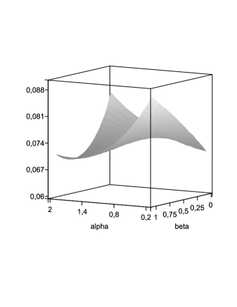
(a) $\widetilde{p}=0.25$, $\widetilde{q}=0.20$

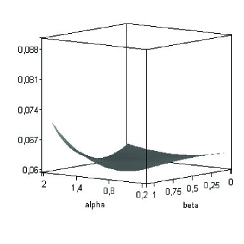
(b) $\widetilde{p}=0.25$, $\widetilde{q}=0.30$

Figure 1: 3D-discrimination plots (49) for $P=\text{Bin}(10,\widetilde{p})$, $Q=\text{Bin}(10,\widetilde{q})$ with $0.2\leq\alpha\leq 2$ and $0\leq\beta\leq 1$.

IV EXPONENTIAL FAMILIES

In this section we show that the scaled Bregman power distances $B_{\alpha}(P,Q\,|\,M)$ can be explicitly evaluated for probability measures $P,\,Q,\,M$ from exponential families. Let us restrict ourselves to the Euclidean observation spaces $(\mathcal{X},\mathcal{A})\subseteq({\mathbb{R}}^{d},{\mathcal{B}}^{d})$ and denote by $x\cdot\theta$ the scalar product of $x,\theta\in{\mathbb{R}}^{d}$. The convex extended real valued function

$$b(\theta)=\ln\int_{{\mathbb{R}}^{d}}e^{x\cdot\theta}\mathrm{d}\lambda(x),\qquad\theta\in{\mathbb{R}}^{d}\,,$$ (50)

and the convex set

$$\Theta=\{\theta\in{\mathbb{R}}^{d}:b(\theta)<\infty\}$$

define on $(\mathcal{X},\mathcal{A})$ an exponential family of probability measures $\{P_{\theta}:\theta\in\Theta\}$ with the densities

$$p_{\theta}(x)\equiv{\frac{\mathrm{d}P_{\theta}}{\mathrm{d}\lambda}}(x)=\exp\{x\cdot\theta-b(\theta)\},\quad x\in{\mathbb{R}}^{d},\quad\theta\in\Theta.$$ (51)

The cumulant function $b(\theta)$ is infinitely differentiable on the interior $\mathring{\Theta}$ with the gradient

$$\bigtriangledown b(\theta)=\left(\frac{\partial}{\partial\theta_{1}},...,\frac{\partial}{\partial\theta_{d}}\right)\,b(\theta)\text{, \ \ \ }\theta\in\mathring{\Theta}.$$

Note that (51) are exponential type densities in the natural form. All exponential type distributions such as Poisson, normal etc. can be transformed to into this form (cf., e.g., Brown (1986)).

The formula

$$\int_{{\mathbb{R}}^{d}}e^{x\cdot\theta}\ \mathrm{d}\lambda(x)\ =\ e^{b(\theta)},\text{ \ \ \ }\theta\in\Theta$$ (52)

follows from (50) and implies

$$\int_{{\mathbb{R}}^{d}}x\,e^{x\cdot\theta}\ \mathrm{d}\lambda(x)\ =\ e^{b(\theta)}\nabla b(\theta),\text{ \ \ \ }\theta\in\mathring{\Theta}.$$ (53)

Both formulas (52) and (53) will be useful in the sequel.

We are interested in the scaled Bregman power distances

$$B_{\alpha}\left(P_{\theta_{1}},P_{\theta_{2}}\,|\,P_{\theta_{0}}\right)\quad\mbox{for}\ \theta_{0},\,\theta_{1},\,\theta_{2}\in\Theta,\ \alpha\in{\mathbb{R}}.$$

Here $P_{\theta_{1}},P_{\theta_{2}},P_{\theta_{0}}$ are measure-theoretically equivalent probability measures, so that we can turn attention to the formulas (39), (30), (33), and (46) to (48), promising to reduce the evaluation of $B_{\alpha}(P_{\theta_{1}},P_{\theta_{2}}\,|\,P_{\theta_{0}})$ to the evaluation of the power divergences $D_{\alpha}(P_{\theta_{1}},P_{\theta_{2}})$. Therefore we first study these divergences and in particular verify their finiteness, which was a sufficient condition for the applicability of the formulas (39), (30) and (33). To begin with, let us mention the following well-established representation:

Theorem 3

If $\alpha\in{\mathbb{R}}$ differs from $0$ and $1$, then the power divergence $D_{\alpha}(P_{\theta_{1}},P_{\theta_{2}})$ is for all $\theta_{1},\,\theta_{2}\in\Theta$  finite and given by the expression

$${\frac{\exp{\big{\{}}b(\alpha\theta_{1}+(1-\alpha)\,\theta_{2})-\alpha b(\theta_{1})-(1-\alpha)\,b(\theta_{2}){\big{\}}}-1}{\alpha(\alpha-1)}\ .}$$

(54)

In particluar, it is invariant with respect to the shifts of the cumulant function linear in $\theta\in\Theta$ in the sense that it coincides with the power divergence $D_{\alpha}(\tilde{P}_{\theta_{1}},\tilde{P}_{\theta_{2}})$ in the exponential family with the cumulant function $\tilde{b}(\theta)=b(\theta)+c+v\cdot\theta$ where $c$ is a real number and $v$ a $d-$vector.

This can be easily seen by slightly extending (38) to get for arbitrary $\alpha\in{\mathbb{R}}$ and $\theta_{1},\,\theta_{2}\in\Theta$

$$1+\alpha\cdot(\alpha-1)\cdot D_{\alpha}(P_{\theta_{1}},P_{\theta_{2}})=\int_{\mathbb{R}^{d}}p_{\theta_{1}}^{\alpha}\,p_{\theta_{2}}^{1-\alpha}\ \mathrm{d}\lambda$$

$$={\frac{\int_{\mathbb{R}^{d}}\exp\{x\cdot[\alpha\theta_{1}+(1-\alpha)\,\theta_{2}]\}\ \mathrm{d}\lambda(x)}{\exp\{\alpha b(\theta_{1})+(1-\alpha)\,b(\theta_{2})\}}}$$

which together with (52) gives the desired result.

The skew symmetry as well as the remaining power divergences $D_{0}(P_{\theta_{1}},P_{\theta_{2}})$ and $D_{1}(P_{\theta_{1}},P_{\theta_{2}})$ are given in the next, straightforward theorem.

Theorem 4

For all $\theta_{1},\,\theta_{2}\in\Theta$ and $\alpha\in{\mathbb{R}}$ different from 0 and 1 there holds

$$D_{\alpha}\left(P_{\theta_{2}},P_{\theta_{1}}\right)\ =\ D_{1-\alpha}\left(P_{\theta_{1}},P_{\theta_{2}}\right)$$

and for $\theta_{2}\in\mathring{\Theta}$

$$D_{-\ln t}\left(P_{\theta_{1}},P_{\theta_{2}}\right)=D_{0}\left(P_{\theta_{1}},P_{\theta_{2}}\right)=\lim_{\alpha\downarrow 0}D_{\alpha}\left(P_{\theta_{1}},P_{\theta_{2}}\right)$$

$$=b(\theta_{1})-b(\theta_{2})-\nabla b(\theta_{2})\,(\theta_{1}-\theta_{2})$$ (55)

$$=\lim_{\alpha\uparrow 1}D_{\alpha}\left(P_{\theta_{2}},P_{\theta_{1}}\right)=D_{1}\left(P_{\theta_{2}},P_{\theta_{1}}\right)=D_{t\ln t}\left(P_{\theta_{2}},P_{\theta_{1}}\right).$$ (56)

The main result of this section is the following representation theorem for Bregman distances in exponential families. We formulate this in terms of the functions

$$\rho_{\alpha}(\theta_{1},\theta_{2})=b\Big{(}\alpha\theta_{1}+(1-\alpha)\,\theta_{2}\Big{)}-\alpha b(\theta_{1})-(1-\alpha)\,b(\theta_{2})$$ (57)

(where the right hand side is finite if $0\leq\alpha\leq 1$), as well as the functions $\sigma_{\alpha}(\theta_{0},\theta_{1},\theta_{2})$ ($\alpha\in\mathbb{R}$, $\theta_{0},\theta_{1},\theta_{2}\in\Theta$) defined as the difference

$$\sigma_{\alpha}(\theta_{0},\,\theta_{1},\,\theta_{2})=\sigma_{\alpha}^{I}(\theta_{0},\,\theta_{1},\,\theta_{2})-\sigma_{\alpha}^{II}(\theta_{0},\,\theta_{1},\,\theta_{2})$$ (58)

of the nonnegative (possibly infinite)

$$\sigma_{\alpha}^{I}(\theta_{0},\,\theta_{1},\,\theta_{2})=b{\Big{(}}\alpha\,\theta_{1}+(1-\alpha)\,\left[\theta_{1}-\theta_{2}+\theta_{0}\right]{\Big{)}}$$ (59)

and the finite

$$\sigma_{\alpha}^{II}(\theta_{0},\,\theta_{1},\,\theta_{2})=\alpha\,b(\theta_{1})+(1-\alpha)\,{\Big{[}}b(\theta_{1})-b(\theta_{2})+b(\theta_{0}){\Big{]}}\ .$$ (60)

Alternatively,

$$\sigma_{\alpha}(\theta_{0},\,\theta_{1},\,\theta_{2})=\rho_{\alpha}(\theta_{1},\theta_{0}+\theta_{1}-\theta_{2})$$

$$+(1-\alpha)\left[b(\theta_{0}+\theta_{1}-\,\theta_{2})-b(\theta_{0})-b(\theta_{1})+b(\theta_{2})\right].$$ (61)

Theorem 5

Let $\theta_{0},\,\theta_{1},\,\theta_{2}\in\Theta$ be arbitrary. If $\alpha(\alpha-1)\neq 0$ then the Bregman distance of the exponential family distributions $P_{\theta_{1}}$ and $P_{\theta_{2}}$ scaled by $P_{\theta_{0}}$ is given by the formula

$$B_{\alpha}\left(P_{\theta_{1}},P_{\theta_{2}}\,|\,P_{\theta_{0}}\right)$$

$$={\frac{\exp\rho_{\alpha}(\theta_{1},\theta_{0})}{\alpha(\alpha-1)}}+{\frac{\exp\rho_{\alpha}(\theta_{2},\theta_{0})}{\alpha}}+\,{\frac{\exp\sigma_{\alpha}(\theta_{0},\theta_{1},\theta_{2})}{1-\alpha}}.$$ (62)

If $\theta_{0}$ respectively $\,\theta_{1}$ is from the interior $\mathring{\Theta}$,  then the limiting Bregman power distances are

$$B_{0}\left(P_{\theta_{1}},P_{\theta_{2}}\,|\,P_{\theta_{0}}\right)$$

$$=\ b(\theta_{1})-b(\theta_{2})-\nabla b(\theta_{0})\,(\theta_{1}-\theta_{2})$$

$$\hskip 12.80365pt+\exp\sigma_{0}(\theta_{0},\theta_{1},\theta_{2})-1$$ (63)

respectively

$$B_{1}\left(P_{\theta_{1}},P_{\theta_{2}}\,|\,P_{\theta_{0}}\right)=b(\theta_{2})-b(\theta_{1})-\nabla b(\theta_{1})\,(\theta_{2}-\theta_{1})\ .$$ (64)

In particluar, all scaled Bregman distances (62) - (64) are invariant with respect to the shifts of the cumulant function linear in $\theta\in\Theta$ in the sense that they coincide with the scaled Bregman distances $B_{\alpha}\left(\tilde{P}_{\theta_{1}},\tilde{P}_{\theta_{2}}\,|\,\tilde{P}_{\theta_{0}}\right)$ in the exponential family with the cumulant function $\tilde{b}(\theta)=b(\theta)+c+v\cdot\theta$ where $c$ is a real number and $v$ a $d-$vector.

Proof

(a)  By (51) it holds for every $\alpha\in{\mathbb{R}}$ and $\theta_{0},\theta_{1},\,\theta_{2}\in\Theta$

$$\left({\frac{p_{\theta_{2}}(x)}{p_{\theta_{0}}(x)}}\right)^{\alpha-1}p_{\theta_{1}}(x)$$

$$=\ \exp{\Big{\{}}(\alpha-1)\big{[}x\cdot(\theta_{2}-\theta_{0})-(b(\theta_{2})-b(\theta_{0}))\big{]}$$

$$\hskip 135.15059pt+x\cdot\theta_{1}-b(\theta_{1}){\Big{\}}}$$

$$=\ \exp{\Big{\{}}x\cdot\big{(}\alpha\,\theta_{1}+(1-\alpha)\,\left[\theta_{1}-\theta_{2}+\theta_{0}\right]\big{)}$$

$$\hskip 126.61467pt-\sigma_{\alpha}^{II}(\theta_{0},\,\theta_{1},\,\theta_{2}){\Big{\}}}$$

with $\sigma_{\alpha}^{II}(\theta_{0},\,\theta_{1},\,\theta_{2})$ from (60). Since (52) leads to

$$\int_{\mathbb{R}^{d}}\exp\Big{\{}x\cdot\Big{(}\alpha\,\theta_{1}+(1-\alpha)\,\left[\theta_{1}-\theta_{2}+\theta_{0}\right]\Big{)}\Big{\}}\,\mathrm{d}\lambda$$

$$=\ \exp\sigma_{\alpha}^{I}(\theta_{0},\,\theta_{1},\,\theta_{2})$$

for $\sigma_{\alpha}^{I}(\theta_{0},\,\theta_{1},\,\theta_{2})$ given by (59), it holds

$$\int_{{\mathcal{X}}}\left({\frac{p_{\theta_{2}}}{p_{\theta_{0}}}}\right)^{\alpha-1}p_{\theta_{1}}\,\mathrm{d}\lambda\ =\ \exp\sigma_{\alpha}(\theta_{0},\theta_{1},\theta_{2})$$ (65)

where $\sigma_{\alpha}(\theta_{0},\theta_{1},\theta_{2})$ was defined in (58). Now, by plugging

$$P=P_{\theta_{1}},\quad Q=P_{\theta_{2}},\quad M=P_{\theta_{0}}\text{ \ \ \ (cf. (\ref{E.1}))}$$

in (39), we get for $\alpha(\alpha-1)\neq 0$ the Bregman distances

$$B_{\alpha}\left(P_{\theta_{1}},P_{\theta_{2}}\,|\,P_{\theta_{0}}\right)$$

$$=\ D_{\alpha}\left(P_{\theta_{1}},P_{\theta_{2}}\right)-(1-\alpha)\,D_{\alpha}\left(P_{\theta_{2}},P_{\theta_{0}}\right)$$

$$\hskip 18.49411pt+\ {\frac{1}{1-\alpha}}\left[\int_{{\mathcal{X}}}\left({\frac{p_{\theta_{2}}}{p_{\theta_{0}}}}\right)^{\alpha-1}p_{\theta_{1}}\,\mathrm{d}\lambda-1\right].$$ (66)

By combining the power divergence formula (54) with (57), one ends up with $D_{\alpha}\left(P_{\theta_{1}},P_{\theta_{2}}\right)={\frac{\exp\{\rho_{\alpha}(\theta_{1},\theta_{2})\}-1}{\alpha(\alpha-1)}}$ which together with (65) and (66) leads to the desired representation (62).

(b)  By the definition of $B_{0}(P,Q\,|\,M)$ in (47) and by (41)

$$B_{0}\left(P_{\theta_{1}},P_{\theta_{2}}\,|\,P_{\theta_{0}}\right)$$

$$=\ D_{0}\left(P_{\theta_{1}},P_{\theta_{0}}\right)-D_{0}\left(P_{\theta_{2}},P_{\theta_{0}}\right)+\int_{{\mathcal{X}}}{\frac{p_{\theta_{0}}\,p_{\theta_{1}}}{p_{\theta_{2}}}}\,\mathrm{d}\lambda-1$$

where

$$\int_{{\mathcal{X}}}{\frac{p_{\theta_{0}}\,p_{\theta_{1}}}{\,p_{\theta_{2}}}}\,\mathrm{d}\lambda\ =\ \exp\sigma_{0}(\theta_{0},\,\theta_{1},\,\theta_{2})\text{ \ (cf. (\ref{E.21})).}$$

For $\theta_{0}\in\mathring{\Theta}$ the desired assertion (63) follows from here and from the formulas

$$D_{0}\left(P_{\theta_{i}},\,P_{\theta_{0}}\right)\ =\ b(\theta_{i})-b(\theta_{0})-\nabla b(\theta_{0})\,(\theta_{i}-\theta_{0})\text{ \ \ for }i=1,2$$

obtained from (55).

(c)  The desired formula (64) follows immediately from the definition (46) and from the formulas (44), (45), (55) and (56).
(d) The finally stated invariance is immediate. $\square$

The Conclusion 1 of Section III about the relation between scaled Bregman distances and $\phi$-divergences can be completed by the following relation between both of them and the classical Bregman distances (1).

Conclusion 2

Let $B_{\phi}(x,y)$ be the classical Bregman distance (1) of $x,y\in\mathbb{R}^{d}$ and $\mathbb{P}=\left\{P_{\theta}:\theta\in\mathbb{R}^{d}\right\}$ the exponential family with cumulant function $\phi$, i.e., with densities $p_{\theta}(s)=\exp\{s\cdot\theta-\phi(\theta)\},$ $s\in\mathbb{R}^{d}$. Then for all $P_{x},P_{y},P_{z}\in\mathbb{P}$

$$B_{\phi}(x,y)=B_{1}(P_{y},P_{x}|P_{z})=D_{1}(P_{y},P_{x})\ ,$$

i.e., there is a one-to-one relation between the classical Bregman distance $B_{\phi}(x,y)$ and the scaled Bregman distances $B_{1}(P_{y},P_{x}|P_{z})$ and power divergences $D_{1}(P_{y},P_{x})$ of the exponential probability measures generated by the cumulant function $\phi$. This means that the family $\left\{B_{\alpha}(P_{y},P_{x}|P_{z}):\alpha\in\mathbb{R},\text{ }z\in\mathbb{R}^{d}\right\}$ of scaled Bregman power distances and the family $\left\{D_{\alpha}(P_{y},P_{x}):\alpha\in\mathbb{R}\right\}$ of power divergences extend the classical Bregman distances $B_{\phi}(x,y)$ to which they reduce at $\alpha=1$ and arbitrary $P_{z}\in\mathbb{P}$. In fact, we meet here the extension of the classical Bregman distances in three different directions: the first represented by various power parameters $\alpha\in\mathbb{R}$, the second represented by various possible exponential distributions parametrized by $\theta\in\mathbb{R}^{d}$, and the third represented by the exponential distribution parameters $z\in\mathbb{R}^{d}$ which are relevant when $\alpha\neq 1$.

Remark 4

We see from Theorems 4 and 5 that – consistent with (30), (45) – for arbitrary interior parameters $\theta_{0},\,\theta_{1},\,\theta_{2}\in\mathring{\Theta}$

$$B_{1}\left(P_{\theta_{1}},P_{\theta_{2}}\,|\,P_{\theta_{0}}\right)=D_{1}\left(P_{\theta_{1}},P_{\theta_{2}}\right),$$

i. e. that the Bregman distance of order $\alpha=1$ of exponential family distributions $P_{\theta_{1}},\,P_{\theta_{2}}$ does not depend on the scaling distribution $P_{\theta_{0}}$. The distance of order $\alpha=0$ satisfies the relation

$$B_{0}\left(P_{\theta_{1}},P_{\theta_{2}}\,|\,P_{\theta_{0}}\right)=D_{0}\left(P_{\theta_{1}},P_{\theta_{2}}\right)+\exp\sigma_{0}(\theta_{0},\,\theta_{1},\,\theta_{2})-1$$

$$=\ B_{1}\left(P_{\theta_{2}},P_{\theta_{1}}\,|\,P_{\theta_{0}}\right)+\Delta(\theta_{0},\,\theta_{1},\,\theta_{2})\ ,$$

where

$$\Delta(\theta_{0},\,\theta_{1},\,\theta_{2})=\exp\sigma_{0}(\theta_{0},\,\theta_{1},\,\theta_{2})-1\vskip 6.0pt plus 2.0pt minus 2.0pt$$

represents a deviation from the skew-symmetry of the Bregman distances $B_{0}\left(P_{\theta_{1}},P_{\theta_{2}}\,|\,P_{\theta_{0}}\right)$ and $B_{1}\left(P_{\theta_{2}},P_{\theta_{1}}\,|\,P_{\theta_{0}}\right)$ of $P_{\theta_{1}}$ and $P_{\theta_{2}}$. This deviation is zero if (for strictly convex $b(\theta)$ if and only if ) $\theta_{0}=\theta_{2}$.

Remark 5

We see from the formulas (54) – (64) that for all $\alpha\in\mathbb{R}$ the quantities $D_{\alpha}\left(P_{\theta_{1}},P_{\theta_{2}}\right)$, $\rho_{\alpha}(\theta_{1},\,\theta_{2})$, $\sigma_{\alpha}(\theta_{0},\,\theta_{1},\,\theta_{2})$ and $B_{\alpha}\left(P_{\theta_{1}},P_{\theta_{2}}\,|\,P_{\theta_{0}}\right)$ only depend on the cumulant function $b(\theta)$ defined in (50), and not directly on the reference measure $\lambda$ used in the definition formulas (50), (51).

V EXPONENTIAL APPLICATIONS

In this section we illustrate the evaluation of scaled Bregman divergences $B_{\alpha}\left(P_{\theta_{1}},P_{\theta_{2}}\,|\,P_{\theta_{0}}\right)$ for some important discrete and continuous exponential families, and also for exponentially distributed random processes.

Binomial model

Consider for fixed $n\geq 2$ on the observation space $\mathcal{X}=\{0,...,n\}$ the binomial distribution $P_{\theta}$ determined by

$$P_{\theta}[\{x\}]=\lambda[\{x\}]\cdot\exp\{x\cdot\theta-b(\theta)\}=\binom{n}{x}p^{x}(1-p)^{n-x}$$

for $x\in\{0,...,n\}$, where

$$\lambda[\{x\}]=\binom{n}{x},\text{\ }\theta=\ln\frac{p}{1-p}\in\Theta=\mathbb{R}\text{\ \ and \ }b(\theta)=n\ln(1+e^{\theta})\ .$$

After some calculations one obtains from (57) and (61)

$$\rho_{\alpha}(\theta_{1},\theta_{2})=n\ln\frac{1+e^{\alpha\theta_{1}+(1-\alpha)\theta_{2}}}{(1+e^{\theta_{1}})^{\alpha}(1+e^{\theta_{2}})^{1-\alpha}}$$

and

$$\sigma_{\alpha}(\theta_{0},\theta_{1},\theta_{2})=n\ln\frac{\left(1+e^{\theta_{1}+(1-\alpha)(\theta_{0}+\theta_{1}-\theta_{2})}\right)(1+e^{\theta_{2}})^{1-\alpha}}{(1+e^{\theta_{0}})^{\alpha}(1+e^{\theta_{1}})}.$$

Applying Theorem 5 one achieves an explicit formula for the binomial Bregman distances $B_{\alpha}\left(P_{\theta_{1}},P_{\theta_{2}}\,|\,P_{\theta_{0}}\right)$ from here.

Rayleigh model

An important role in communication theory play the Rayleigh distributions defined by the probability densities

$$p_{\theta}(x)=\theta x\exp\left\{-\frac{\theta x^{2}}{2}\right\},\text{ \ }\theta\in\Theta=(0,\infty)$$ (67)

with respect to the restriction $\lambda_{+}$ of the Lebesgue measure $\lambda$ on the observation space $\mathcal{X}=(0,\infty).$ The mapping

$$T(x)=-\sqrt{2x}$$

from the positive halfline $(0,\infty)$ to the negative halfline $(-\infty,0)$ transforms (67) into the family of Rayleigh densities

$$p_{\theta}(x)=\theta\exp\left\{\theta x\right\}=\exp\left\{\theta x-b(\theta)\right\}$$

$$\hskip 113.81102pt\text{ \ for }b(\theta)=-\ln\theta,\text{ }\theta>0$$

with respect to the restriction $\lambda_{-}$ of the Lebesgue measure $\lambda$ on the observation space $\mathcal{X}=(-\infty,0).$ These are the Rayleigh densities in the natural form assumed in (51). After some calculations one derives from (57)

$$\rho_{\alpha}(\theta_{1},\theta_{2})=\ln\frac{\theta_{1}^{\alpha}\,\theta_{2}^{1-\alpha}}{\alpha\theta_{1}+(1-\alpha)\theta_{2}}$$ (68)

and

$$\sigma_{\alpha}(\theta_{0},\theta_{1},\theta_{2})=\ln\frac{\theta_{1}\text{ }\theta_{0}^{1-\alpha}}{\left(\alpha\theta_{1}+(1-\alpha)(\theta_{0}+\theta_{1}-\theta_{2})\right)\text{ }\theta_{2}^{1-\alpha}}.$$

Applying Theorem 5 one obtains the Rayleigh-Bregman distances $B_{\alpha}\left(P_{\theta_{1}},P_{\theta_{2}}\,|\,P_{\theta_{0}}\right)$ from here.

Theorem 1 about the preservation of the scaled Bregman distances by statistically sufficient transformations is useful for the evaluation of these distances in exponential families. It implies for example that these distances in the normal and lognormal families coincide. The next two examples dealing with distances of stochastic processes make use of this theorem too.

Exponentialy distributed signals

Most of the random processes modelling physical, social and economic phenomena are exponentially distributed. Important among them are the real valued Lévy processes $\boldsymbol{X}\boldsymbol{X}_{t}=(X_{s}:0\leq s\leq t)$ with trajectories $\boldsymbol{x}\boldsymbol{x}_{t}=(x_{s}:0\leq s\leq t)$ from the Skorokchod observation spaces $(\mathcal{X}_{t},\mathcal{A}_{t})$ and parameters from the set

$$\Theta=\{\theta\in\mathbb{R}:c(\theta)<\infty\}$$

defined by means of the function

$$c(\theta)=\int_{\mathbb{R}\backslash\{0\}}x^{2}e^{\theta x}/(1+x^{2})\,\mathrm{d}\nu(x)$$

where $\nu$ is a Lévy measure which determines the probability distribution of the size of jumps of the process and the intensity with which jumps occur. It is assumed that $0$ belongs to $\Theta$ and it is known (cf., e.g., Küchler and Sorensen (1994)) that the probability distributions $P_{t,\theta}$ induced by these processes on $(\mathcal{X}_{t},\mathcal{A}_{t})$ are mutually measure-theoretically equivalent with the relative densities

$$\frac{\mathrm{d}P_{t,\theta}}{\mathrm{d}P_{t,0}}(\boldsymbol{x}\boldsymbol{x}_{t})=\exp\{\theta\text{ }x_{t}-b_{t}(\theta)\}$$ (69)

for the end $x_{t}$ of the trajectory $\boldsymbol{x}\boldsymbol{x}_{t}$. The cumulant function appearing here is

$$b_{t}(\theta)=t\left(\delta\theta+\frac{1}{2}\sigma^{2}\theta^{2}+\gamma(\theta)\right)$$ (70)

for two genuine parameters $\delta\in\mathbb{R}$ respectively $\sigma>0$ of the process which determine its intensity of drift respectively its volatility, and for the function

$$\gamma(\theta)=\int_{\mathbb{R}\backslash\{0\}}[e^{\theta x}-1-\theta x/(1+x^{2})]\,\mathrm{d}\nu(x).$$

The formula (69) implies that the family $\mathbb{P}_{t}$ $=\{P_{t,\theta}:\theta\in\Theta\}$ is exponential on $(\mathcal{X}_{t},\mathcal{A}_{t})$ for which the “extremally reduced” observation $T(\boldsymbol{x}\boldsymbol{x}_{t})=x_{t}$ is statistically sufficient. Thus, by Theorem 1,

$$B(P_{t,\theta_{1}},P_{t,\theta_{2}}|P_{t,0})=B(Q_{t,\theta_{1}},Q_{t,\theta_{2}}|Q_{t,0})$$ (71)

where $Q_{t,\theta}$ is a probability distribution on the real line governing the marginal distribution of the last observed value $X_{t}$ of the process $\boldsymbol{X}\boldsymbol{X}_{t}$.

Queueing processes and Brownian motions

For illustration of the general result of the previous subsection we can take the family of Poisson processes with initial value $X_{0}=0$ and intensities $\eta=e^{\theta},\ \theta\in\Theta=\mathbb{R}\$ for which $\delta=\sigma=0$ and $c(\theta)=e^{\theta}-1$ so that $b_{t}(\theta)=t\left(e^{\theta}-1\right).$ Then $Q_{t,\theta}$ is the Poisson distribution $\text{Poi}(\tau)$ with parameter $\tau=t\eta=te^{\theta}$ and probabilities

$$Q_{t,\theta}[\{x\}]=\frac{e^{-\tau}\left(\tau\right)^{x}}{x!}=\lambda[\{x\}]\cdot\exp\left\{x\vartheta-e^{\vartheta}\right\}$$

$$\hskip 56.9055pt\text{ \ for \ }\vartheta=\ln\tau=\theta+\ln t,\ \ \lambda[\{x\}]=\frac{1}{x!}\ .$$

The exponential structure is similar as above, so that by applying (57) to the cumulant function $b(\vartheta)=e^{\vartheta}=te^{\theta}$ we get for the Poisson processes with parameters $\theta_{1}$ and $\theta_{2}$

$$\rho_{\alpha}(\theta_{1},\theta_{2})=t\left[e^{\alpha\theta_{1}+(1-\alpha)\theta_{2}}-\alpha e^{\theta_{1}}-(1-\alpha)e^{\theta_{2}}\right].$$

Combining this with (61) and Theorem 5 we obtain an explicit formula for the scaled Bregman distance (71) of these Poisson processes.

To give another illustration of the result of the previous subsection, let us first introduce the standard Wiener process $\widetilde{X}_{t}$ which is the Lévy process with $\nu\equiv 0$, $\delta=0$, $\sigma=1$ and $\theta=1$. It defines the family of Wiener processes

$$X_{s}=\theta\,\widetilde{X}_{s},\text{ \ \ }0\leq s\leq t,\ \ \theta\in(0,\infty),$$

which are Lévy processes with $\delta=0$, $\sigma=1$ and $c(\theta)\equiv 0$ so that (70) implies $b_{t}(\theta)=\theta^{2}/2.$ They are well-known models of the random fluctuations called Brownian motions. If the initial value $X_{0}$ is zero then $Q_{t,\theta}$ is the normal distribution with mean zero and variance $v^{2}=t\theta^{2}$. The corresponding Lebesgue densities

$$\frac{1}{\sqrt{2\pi v^{2}}}\exp\left\{-\frac{x^{2}}{2v^{2}}\right\}=\sqrt{\frac{\vartheta}{\pi}}\exp\left\{-\vartheta x^{2}\right\}\text{ \ for }\vartheta=\frac{1}{2v^{2}}\text{\ }$$

are transformed by the mapping $x\longmapsto-\sqrt{|x|}$ of $\mathbb{R}$ on the negative halfline $(-\infty,0)$ into the natural exponential densities $\exp\left\{\vartheta x-b(\vartheta)\right\}$ with respect to the dominating density $1/\sqrt{\pi|x|}$ where $b(\vartheta)=-\frac{1}{2}\ln\vartheta=-\ln\frac{1}{\theta}+\frac{1}{2}\ln 2t.$ Thus by (57)

$$\rho_{\alpha}(\theta_{1},\theta_{2})=-\ln\frac{\theta_{1}^{\alpha}\,\theta_{2}^{1-\alpha}}{\alpha\theta_{1}+(1-\alpha)\theta_{2}}\qquad(cf.\ (\ref{ro})).$$

This together with (61) and Theorem 5 leads to the explicit formula for the scaled Bregman distance (71) of the Wiener processes under consideration.

Geometric Brownian motions

From the abovementioned standard Wiener process one can also build up the family of geometric Brownian motions (geometric Wiener processes)

$$Y_{s}=\exp\{\sigma\widetilde{X}_{s}+\theta s\},\text{ \ \ }0\leq s\leq t,\ \ \theta\in\mathbb{R},$$

where the family-generating $\theta$ can be interpreted as drift parameters, and the volatility parameter $\sigma>0$ is assumed to be constant all over the family. Then, $\sigma\widetilde{X}_{t}+\theta t$ is normally distributed with mean $m=\theta t$ and variance $v^{2}=\sigma^{2}t$, and $Y_{t}$ is lognormally distributed with the same parameters $m$ and $v^{2}$. By (71), the scaled Bregman distance of two geometric Brownian motions with parameters $\theta_{1}$, $\theta_{2}$ reduces to the scaled Bregman distance of two lognormal distributions LN($\theta_{1}t,\sigma^{2}t),$ LN($\theta_{2}t,\sigma^{2}t).$ As said above, it coincides with the scaled Bregman distance of two normal distributions N($\theta_{1}t,\sigma^{2}t),$ N($\theta_{2}t,\sigma^{2}t).$ This is seen also from the fact that the reparametrization

$$\vartheta=\frac{\mu}{v^{2}},\text{ \ }\tau=\frac{1}{2v^{2}}$$

and transformations $\mathbb{R}\longmapsto\mathbb{R}^{2}$ similar to that from the previous example lead in both distributions N($\mu,v^{2}$) and LN($\mu,v^{2}$) to the same natural exponential density

$$p_{\vartheta,\tau}(x_{1},x_{2})=\exp\left\{x_{1}\vartheta+x_{2}\tau-b(\vartheta,\tau)\right\}$$

with

$$b(\vartheta,\tau)=\frac{1}{2}\,\ln\tau+\frac{\vartheta^{2}}{4\tau}.$$

These two distributions differ just in the dominating measures on the transformed observation space $\mathcal{X=}$ $\mathbb{R}^{2}$. For $(\mu_{1},v_{1}^{2})=(\theta_{1}t,\sigma^{2}t)$  and  $(\mu_{2},v_{2}^{2})=(\theta_{2}t,\sigma^{2}t)$ we get

$$(\vartheta_{1},\tau_{1})=\left(\frac{\theta_{1}}{\sigma^{2}}\,,\,\frac{1}{2\sigma^{2}t}\right)\text{ \ and \ }(\vartheta_{2},\tau_{2})=\left(\frac{\theta_{2}}{\sigma^{2}}\,,\,\frac{1}{2\sigma^{2}t}\right)$$

and thus

$$b(\alpha(\vartheta_{1},\tau_{1})+(1-\alpha)(\vartheta_{2},\tau_{2}))-\alpha b(\vartheta_{1},\tau_{1})-(1-\alpha)b(\vartheta_{2},\tau_{2})$$

$$=\frac{\left(\alpha\theta_{1}+(1-\alpha)\theta_{2}\right)^{2}-\alpha\theta_{1}^{2}+(1-\alpha)\theta_{2}^{2}}{2\sigma^{2}}\ t\ .$$

Hence, for distributions $P_{t,\theta_{1}},$ $P_{t,\theta_{2}}$ of the geometric Brownian motions considered above we get from (57)

$$\rho_{\alpha}(\theta_{1},\theta_{2})=\frac{\left[\left(\alpha\theta_{1}+(1-\alpha)\theta_{2}\right)^{2}-\alpha\theta_{1}^{2}+(1-\alpha)\theta_{2}^{2}\right]}{2\sigma^{2}}\ t\ .$$

The expression (61) can be automatically evaluated using this. Applying both these results in Theorem 5 one obtains explicit formula for the scaled Bregman distance (71) of these geometric Brownian motions.

References

Amari S.-I. (2007), “Integration of stochastic models by minimizing $\alpha$-divergence,” Neural Computation, vol. 19, no. 10, pp. 2780-2796.

Banerjee, A., Guo, X., and Wang, H. (2005a), “On the optimality of conditional expectation as a Bregman predictor, ” IEEE Transaction on Information theory, vol. 51, no. 7, pp. 2664-2669.

Banerjee, A., Merugu, S., Dhillon, I.S. and Ghosh, J. (2005b), “Clustering with Bregman divergences,” J. Machine Learning Research, vol. 6, pp. 1705-1749.

Bartlett, P.L., Jordan M.I. and McAuliffe, J.D. (2006), “Convexity, classification and risk bounds,” JASA, vol. 101,pp. 138-156.

Bauschke, H.H. and Borwein, J.M. (1997), “Legendre functions and the method of random Bregman projections, ” J. Convex Analysis, vol. 4, No. 1, pp. 27-67.

Boratynska, A. (1997), “Stability of Bayesian inference in exponential families,” Statist. & Probab. Letters, vol. 36, pp. 173-178.

Bregman, L.M. (1967), “The relaxation method of finding the common point of convex sets and its application to the solution of problems in convex programming,” USSR Computational Mathematics and Mathematical Physics, vol. 7, no. 3, pp. 200-217.

Brown, L.D. (1986), Fundamentals of Statistical Exponential Families. Hayward, California: Inst. of Math. Statistics.

Butnariu, D. and Resmerita, E. (2006), “Bregman distances, totally convex functions, and a method for solving operator equations in Banach spaces, ” Abstr. Appl. Anal., vol. 2006, Art. ID 84919, 39 pp.

Byrne, C. (1999), “Iterative projection onto convex sets using multiple Bregman distances,” Inverse Problems, vol. 15, pp. 1295-1313.

Carlson, B.A. and Clements, M.A. (1991), “A computationally compact divergence measure for speech processing. IEEE Transactions on PAMI, vol. 13, pp. 1255-1260.

Censor, Y. and Zenios, S.A. (1997), Parallel Optimization - Theory, Algorithms, and Applications. New York: Oxford University Press.

Cesa-Bianchi, N. and Lugosi, G. (2006), Prediction, Learning, Games. Cambridge: Cambridge University Press.

Collins, M., Schapire, R.E. and Singer, Y. (2002), “Logistic regression, AdaBoost and Bregman distances,” Machine Learning, vol. 48, pp. 253-285.

Csiszár, I. (1963), “Eine informationstheoretische Ungleichung und ihre Anwendung auf den Beweis der Ergodizität von Markoffschen Ketten. Publ. Math. Inst. Hungar. Acad. Sci., ser. A, vol. 8, pp. 85-108.

Csiszár, I. (1967), “Information-type measures of difference of probability distributions and indirect observations. Studia Sci. Math. Hungar., vol. 2, pp. 299-318.

Csiszár, I. (1991), “Why least squares and maximum entropy? An axiomatic approach to inference for linear inverse problems,” Annals of Statistics, vol. 19, no. 4, pp. 2032-2066.

Csiszár, I. (1994), “Maximum entropy and related methods,”  Trans. 12th Prague Conf. Information Theory, Statistical Decision Functions and Random Processes. Prague, Czech Acad. Sci., pp. 58-62.

Csiszár, I. (1995), “Generalized projections for non-negative functions,” Acta Mathematica Hungarica, vol. 68, pp. 161-186.

Csiszár, I. and Matúš, F. (2008), “On minimization of entropy functionals under moment constraints,” Proceedings of ISIT 2008, Toronto, Canada, pp. 2101-2105.

Csiszár, I. and Matúš, F. (2009), “On minimization of multivariate entropy functionals,” Proceedings of ITW 2009, Volos, Greece, pp. 96-100.

Do, M.N. and Vetterli, M. (2002), “Wavelet-based texture retrieval using generalized Gaussian density and Kullback-Leibler distance,”  IEEE Transactions on Image Processing, vol. 11, pp. 146-158.

Freund, Y. and Schapire, R.E. (1997), “A decision-theoretic generalization of on-line learning and an application to boosting,”  J. Comput. Syst. Sci., vol. 55, pp. 119-139.

Halmos, P.R. (1964), Measure Theory. New York: D. Van Nostrand.

Hertz, T., Bar-Hillel, A. and Weinshall, D. (2004), “Learning distance functions for information retrieval,” in Proc. IEEE Comput. Soc. Conf. on Computer Vision and Pattern Rec. CVPR, vol. 2, II-570 - II-577.

Jones, L.K. and Byrne, C.L. (1990), “General entropy criteria for inverse problems, with applications to data compression, pattern classification, and cluster analysis,” IEEE Trans. Inform. Theory vol. 36, no. 1, pp. 23-30.

Küchler, U. and Sorensen, M. (1994), “Exponential families of stochastic processes and Lévy processes,” J. of Statist. Planning and Inference, vol. 39, pp. 211-237.

Lehman, E.L. and Romano J.P. (2005), Testing Statistical Hypotheses. Berlin: Springer.

Liese, F. and Vajda, I. (1987), Convex Statistical Distances. Leipzig: Teubner.

Liese, F. and Vajda, I. (2006), “On divergences and informations in statistics and information theory,” IEEE Transaction on Information theory, vol. 52, no. 10, pp. 4394-4412.

Lloyd, S.P. (1982), “Least squares quantization in PCM,” IEEE Transactions on Inform. Theory, vol. 28, no. 2, pp. 129-137.

Marquina, A. and Osher, S.J. (2008), “Image super-resolution by TV-regularization and Bregman iteration,” J. Sci. Comput., vol. 37, pp. 367-382.

Murata, N., Takenouchi, T., Kanamori, T. and Eguchi, S. (2004), “Information geometry of $\mathcal{U}$-Boost and Bregman divergence,”  Neural Computation, vol. 16, no. 7, pp. 1437-1481.

Nock, R. and Nielsen, F. (2009), “Bregman divergences and surrogates for learning,” IEEE Transactions on PAMI, vol. 31, no. 11, pp. 2048 - 2059.

Pardo, M.C. and Vajda, I. (1997), “About distances of discrete distributions satisfying the data processing theorem of information theory,” IEEE Transaction on Information theory, vol. 43, no. 4, pp. 1288-1293.

Pardo, M.C. and Vajda, I. (2003), “On asymptotic properties of information-theoretic divergences,” IEEE Transaction on Information theory, vol. 49, no. 7, pp. 1860-1868.

Rényi, A. (1961), “On measures of entropy and information,” in Proc. 4th Berkeley Symp. Math. Stat. Probab., vol. 1, pp. 547-561. Berkeley, CA: Univ. of California Press.

Resmerita, E. and Anderssen R.S. (2007), “Joint additive Kullback-Leibler residual minimization and regularization for linear inverse problems,” Math. Meth. Appl. Sci., vol. 30, no. 13, pp. 1527-1544.

Scherzer, O., Grasmair, M., Grossauer, H., Haltmeier, M. and Lenzen, F. (2008); Variational methods in imaging. New York: Springer.

Stummer, W. (2007), “Some Bregman distances between financial diffusion processes,” Proc. Appl. Math. Mech., vol. 7, no. 1, pp. 1050503 - 1050504.

Stummer, W. and Vajda, I. (2010), “On divergences of finite measures and their applicability in statistics and information theory,”  Statistics, vol. 44, pp. 169-187.

Teboulle, M. (2007), “A unified continuous optimization framework for center-based clustering methiods,” Journal of Machine Learning Research, vol. 8, pp. 65-102.

Vajda, I. (2009), “ On metric divergences of probability measures,” Kybernetika, vol. 45, no. 5 (in print).

Vajda, I. and Zvárová, J. (2007), “On generalized entropies, Bayesian decisions and statistical diversity,” Kybernetika, vol. 43, no. 5, pp. 675-696.

Veldhuis, R.N.J. (2002), “The centroid of the Kullback-Leibler distance,” IEEE Signal Processing Letters, vol. 9, no. 3, pp. 96-99.

Xu, J. and Osher, S. (2007), “Iterative regularization and nonlinear inverse scale space applied to wavelet-based denoising,” IEEE Transaction on Image Processing, vol. 16, no. 2, pp. 534-544.

Wolfgang Stummer graduated from the Johannes Kepler University Linz, Austria, in 1987 and received the Ph.D. degree in 1991 from the University of Zurich, Switzerland.
From 1993 to 1995 he worked as Research Assistant at the University of London and the University of Bath (UK). From 1995 to 2001 he was Assistant Professor at the University of Ulm (Germany). From 2001 to 2003 he held a Term Position as a Full Professor at the University of Karlsruhe (now KIT; Germany) where he continued as Associate Professor until 2005. Since then, he is affiliated as Full Professor at the Department of Mathematics, University of Erlangen-Nürnberg FAU (Germany); at the latter, he is also a Member of the School of Business and Economics.

Igor Vajda (M 90 - F 01) was born in 1942 and passed away suddenly after a short illness on May 2, 2010. He graduated from the Czech Technical University, Czech Republic, in 1965 and received the Ph.D. degree in 1968 from Charles University, Prague, Czech Republic.
He worked at UTIA (Institute of Information Theory and Automation, Czech Academy of Sciences) from his graduation until his death, and became a member of the Board of UTIA in 1990. He was a visiting professor at the Katholieke Universiteit Leuven, Belgium; the Universidad Complutense Madrid, Spain; the Université de Montpellier, France; and the Universidad Miguel Hérnandez, Alicante, Spain. He published four monographs and more than 100 journal publications.
Dr.  Vajda received the Prize of the Academy of Sciences, the Jacob Wolfowitz Prize, the Medal of merits of Czech Technical University, several Annual prizes from UTIA, and, posthumously, the Bolzano Medal from the Czech Academy of Sciences.