The orientations of galaxy groups and formation of the Local Supercluster.

Abstract

We analysed the orientation of galaxy groups in the Local Supercluster (LSC). It is strongly correlated with the distribution of neighbouring groups in the scale till about 20 Mpc. The group major axis is in alignment with both the line joining the two brightest galaxies and the direction toward the centre of the LSC, i.e. Virgo cluster. These correlations suggest that two brightest galaxies were formed in filaments of matter directed towards the protosupercluster centre. Afterwards, the hierarchical clustering leads to aggregation of galaxies around these two galaxies. The groups are formed on the same or similarly oriented filaments. This picture is in agreement with the predictions of numerical simulations.

1 Introduction

Binggeli (1982) was the first who found that major axes of galaxy clusters tend to point towards their neighbours. Later the existence of this effect was discussed by several authors and usually the significant alignment was reported. The distance between clusters for which the effect was detected changed from $10h^{-1}Mpc$ till $150h^{-1}Mpc$ (where $h=H_{0}/100\,km\,s^{-1}Mpc^{-1}$). The strength of the effect decreases with distance (Struble & Peebles, 1985; Flin, 1987; Rhee & Katgert, 1987; Ulmer et al., 1989; Plionis, 1994; West, 1989; Chambers et al., 2000; Hashimoto et al., 2008). These investigations involved both optical and X-ray data, as well as clusters belonging (or not) to superclusters. Nowadays, it is accepted that the effect is not due to selection effects but is real and its distance scale is between $10-60h^{-1}Mpc$. The alignment of galaxy group was studied by West (1995). He used CfA group catalog (Geller & Huhra, 1983) and a catalog based on SSRS ( Southern Sky Redshit Survey) (Maia et al., 1989). Each group should have at least $4$ objects and less than $100$. Decontamination of the groups by foreground and background objects was performed by removing objects with redshift difference from the group mean over $1000\,km\,s^{-1}$. They were $59$ groups and Binggeli effect was observed among galaxy groups till $15-30h^{-1}Mpc$. One should note that the investigation of galaxy group orientation is more difficult than in the case of galaxy clusters. The position angle of a group consisting of a few objects is determined with much greater error than for rich clusters. Moreover, statistics with small number are less reliable. The other investigations of galaxy groups were performed by Palumbo et al. (1993). During study the orientation of $92$ out of $100$ compact groups listed in the Catalogue of the Compact Groups (Hickson, 1982), they do not find alignment, but location of groups along long chains is noted.

The interpretation of the effect has changed with development of theories, but the main idea that this should reflect conditions during the structure formation is still very popular. Numerical simulations gave a better understanding of physical processes leading to structure formation. These simulations were performed in the framework of the cold dark matter (CDM) model presently regarded as the correct description of the large scale structure formation. Using different approaches and codes, these investigations led to the conclusion that the preferred orientation of galaxy clusters in the CDM model is a natural consequence of processes leading to structure formation due to gravitational interaction. Onuora & Thomas (2000) using large - scale simulation found that in $\Lambda$CDM cosmological model effect reaches the distance up to $30Mpc$, while in $\tau$CDM model the range of effects is twice smaller. Also in SCDM and OCDM models, where smaller scale simulations were performed, some alignment effect could be noted. N - body simulation for standard $\Lambda$CDM model (Faltenbacher et al., 2002) for $3000$ clusters showed the alignment of neighbouring clusters in the distance range from $10-15Mpc$, while the Binggeli effect till about $100Mpc$ is observed. The strong alignment, decreasing with the increasing distance between clusters, observed till about 100 Mpc was reported (Hopkins et al., 2005). The preferred orientation of clusters belonging to superclusters existed also in SHM + N body simulation . Moreover, from some of the numerical simulations, it follows that the structure formation occurred along filamentary structures rather than the walls (Faltenbacher et al., 2005; Springel et al., 2005; Binggeli, 1982; Hahn et al., 2007a, b; Aragon-Calvo, 2007; van de Weygaert & Bond, 2008a, b). In order to confirm, or deny, this scheme of structure origin we carry out an analysis of the Local Supercluster (LSC) galaxy groups alignment as well as the distribution of the acute angle between the position angle of the structure and the direction to all remaining clusters. Groups were taken from Nearby Galaxies (NBG) Catalog (Tully, 1988). We investigated also the alignment of the brightest group galaxy and the parent group. We determined the position of the line joining the two brightest galaxies and checked the orientation of this line in respect to parent group and direction towards Virgo cluster. The distributions of these angles, as well as differences between some of these angles were tested for isotropy.

The paper is organised in the following manner. Section 2 describes observational data, section 3 presents statistical method used in the paper, section 4 presents results and discussions. In section 5 we formulate conclusions.

2 Observational data

In the present paper we study the alignment of galaxy groups. Groups were taken from NBG Catalog (Tully, 1988). This Catalog contains 2367 galaxies with radial velocities less than $3000\,km\,s^{-1}$. It is complete till magnitude limit $B^{b,i}_{T}=12.0$ and moreover dimmer, low-surface brightness gas reach galaxies (late type spirals) are also incorporated, which ensure that all more massive galaxies are taken into account. Due to our position in the LSC it is complete for such objects till the Virgo Cluster centre. An important point is that this Catalog provides the uniform coverage of entire unobscured sky (Tully, 1987) and only more massive galaxies are taken into account. Moreover, the the galaxy distances are very well and in uniform manner determined. The galaxy distance are based on velocities, assuming the flat cosmological model ($q_{0}=1/2$) with $H_{0}=75km\,s^{-1}Mpc^{-1}$ and the model describing velocity perturbations in the vicinity of the Virgo Cluster (Tully & Shaya, 1984). Galaxies position angles were taken from Nilson (1973, 1974); Lauberts (1982); Lauberts & Valentijn (1989), and for 7 missing measurements they were made on PSS prints by the present authors.

The NBG Catalog gives also the affiliation of galaxies to groups. Groups were found using precise criteria. In our opinion the groups extracted from the NBG Catalog (Tully, 1988) are very good observational basis for study of their properties.

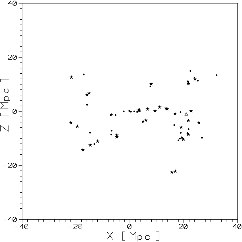
Figure 1: The spatial distribution of galaxy groups in the LSC, Dots - groups with 10- 20 members, stars - more than 20 member galaxies, triangle - Virgo Cluster centre. On the left panel we present projection into X-Y plane, while on the right X-Z projection is presented. The coordinate of the Earth are [0,0].

From the Tully’s Catalog we extracted aggregation of galaxies having at least 40 members, which ensures that at least one substructure has 10 or more members. The substructure having at least 10 members were taken for the analysis and we call them groups. We decided to select structures having at least 10 objects, because the determination of structure great axis is reliable in this case (see also West (1989)). There are $61$ such groups. Moreover, we repeated the analysis for subsample containing $35$ groups having at least $20$ galaxies (Fig.1).

It was assumed that groups are two axial ellipsoids. The shape of each group has been determined considering only the projected position of galaxies on the celestial sphere in the supergalactic coordinate system $L$, $B$ and applying the covariance ellipse method. This procedure gives the position angle of the group major axis.

The position angle of each group $PA_{g}$ is calculated counterclockwise from the great circle passing through the position of the group centre on the celestial sphere and the northern pole of the LSC. It was assumed that the location of a group centre corresponds to the mean of $L$ and $B$ coordinates of member galaxies and the mean of radial velocity, as given in the Catalog. Using standard formula from spherical trigonometry, we calculated the directions between the centre of each group and the centres of the remaining groups. Each direction is a part of the great circle joining the centres of two groups. For each group we calculated the acute angle $\phi$ between the position angle of the major axis of a given group $PA_{g}$ and direction towards other groups. In such a manner we have $3660$ directions among groups. We also investigated the alignment of the brightest group galaxy $PA_{bm}$ and the parent group $PA_{g}$. Moreover, we determined the position of the line joining two brightest galaxies in the group $PA_{l}$ and checked the orientation of this line relative to the position angle of the parent group $PA_{g}$, the position angle of the brightest galaxy $PA_{bm}$ and the direction towards Virgo cluster $PA_{V}$. The projected two dimensional line between two groups is used to compute the acute angle $\phi$

3 Statistics

3.1 The general view

We checked for isotropy four discussed distributions of position angles ($PA_{g}$, $PA_{l}$, $PA_{bm}$, $PA_{V}$) having range $0^{o}$- $180^{o}$, as well as differences between position angles ($PA_{g}-PA_{V}$, $PA_{l}-PA_{V}$, $PA_{g}-PA_{l}$, $PA_{bm}-PA_{g}$, $PA_{bm}-PA_{l}$, $PA_{bm}-PA_{V}$) being the acute angles. Theoretically, the range of the angles $PA_{V}$ and $PA_{l}$ is between $0^{o}$ and $360^{o}$, whereas the range of two remaining angles $PA_{g}$ and $PA_{bm}$ is restricted to the range $0^{o}$-$180^{o}$. We are studding the difference between direction of angles. In such analysis, for $PA_{V}$ and $PA_{l}$ an angle $\zeta$ and $\zeta+180^{o}$ are identical.

The detailed statistical analysis was done using the Fourier test (Hawley & Peebles, 1975; Flin & Godłowski, 1986; Kindl, 1987; Godłowski, 1993, 1994), Kolmogorov - Smirnov test and the $\chi^{2}$ test. Additionally, we carried out the analysis of these angles for subsample of 35 groups having at least 20 members. In all cases the entire range of the analysed angles (position angles and differences between position angles) was divided into n equal width bins. In the following analysis we divided the range of analysed angles into bins of $15$ degrees width, which gives $12$ bins in the case of position angles and $6$ in the case of differences between position angles. Let us denote the total number of analysed groups as $N$, the number of groups with analysed angles within k-th angular bin as $N_{k}$ and $N_{0}$ as mean number of groups per bin.

3.2 $\chi^{2}$ test

The dividing range of the analysed angle into $n$ equal width bins, gives $n-1$ degrees of freedom in the $\chi^{2}$ test. The value of the $\chi^{2}$ statistics is given by the formula

$$\chi^{2}=\sum_{k=1}^{n}{(N_{k}-N_{0})^{2}\over N_{0}}.$$ (1)

The $\chi^{2}$ test yields at the significance level $\alpha=0.05)$ the critical value of $19.7$ for $11$ degrees of freedom at the significance level $\alpha=0.05)$ and $11.1$ for $5$ degrees of freedom.

3.3 The Fourier test

If deviation from isotropy is a slowly varying function of the angle $\theta$ one can use the Fourier test

$$N_{k}=N_{0,k}(1+\Delta_{11}\cos{2\theta_{k}}+\Delta_{21}\sin{2\theta_{k}})$$ (2)

where $N_{0,k}$ are expected number of groups per bin (in our case all $N_{0,k}$ are equal).

We obtain the following expression for the $\Delta_{i1}$ coefficients

$$\Delta_{11}={\sum_{k=1}^{n}(N_{k}-N_{0,k})\cos{2\theta_{k}}\over\sum_{k=1}^{n}N_{0,k}\cos^{2}{2\theta_{k}}}$$ (3)

$$\Delta_{21}={\sum_{k=1}^{n}(N_{k}-N_{0,k})\sin{2\theta_{k}}\over\sum_{k=1}^{n}N_{0,k}\sin^{2}{2\theta_{k}}}$$ (4)

with the standard deviation given by expressions:

$$\sigma(\Delta_{11})=\left({\sum_{k=1}^{n}N_{0,k}\cos^{2}{2\theta_{k}}}\right)^{-1/2}=\left({2\over nN_{0}}\right)^{1/2},$$ (5)

$$\sigma(\Delta_{21})=\left({\sum_{k=1}^{n}N_{0,k}\sin^{2}{2\theta_{k}}}\right)^{-1/2}=\left({2\over nN_{0}}\right)^{1/2}.$$ (6)

The probability that the amplitude

$$\Delta_{1}=\left(\Delta_{11}^{2}+\Delta_{21}^{2}\right)^{1/2}$$ (7)

is greater than a certain chosen value is given by the formula

$$P(>\Delta_{1})=\exp{\left(-{n\over 4}N_{0}\Delta_{1}^{2}\right)}$$ (8)

with standard deviation of this amplitude

$$\sigma(\Delta_{1})=\left({2\over nN_{0}}\right)^{1/2}.$$ (9)

This test was originally introduced by Hawley & Peebles (1975) and substantially modified by Godłowski (1994) for the case when taking into account higher Fourier modes:

$$N_{k}=N_{0,k}(1+\Delta_{11}\cos{2\theta_{k}}+\Delta_{21}\sin{2\theta_{k}}+\Delta_{12}\cos{4\theta_{k}}+\Delta_{22}\sin{4\theta_{k}}+.....).$$ (10)

In our case (all $N_{0,k}$ are equal) it leads to formulas for the $\Delta_{ij}$ coefficients:

$$\Delta_{1j}={\sum_{k=1}^{n}N_{k}\cos{2J\theta_{k}}\over\sum_{k=1}^{n}N_{0}\cos^{2}{2J\theta_{k}}},$$ (11)

and

$$\Delta_{2j}={\sum_{k=1}^{n}N_{k})\sin{2J\theta_{k}}\over\sum_{k=1}^{n}N_{0}\sin^{2}{2J\theta_{k}}},$$ (12)

with the standard deviation

$$\sigma(\Delta_{11})=\left({\sum_{k=1}^{n}N_{0}\cos^{2}{2\theta_{k}}}\right)^{-1/2}=\left({2\over nN_{0}}\right)^{1/2},$$ (13)

and

$$\sigma(\Delta_{21})=\left({\sum_{k=1}^{n}N_{0}\sin^{2}{2\theta_{k}}}\right)^{-1/2}=\left({2\over nN_{0}}\right)^{1/2}.$$ (14)

If we analysed Fourier modes separately, probability that the amplitude

$$\Delta_{j}=\left(\Delta_{1j}^{2}+\Delta_{2j}^{2}\right)^{1/2}$$ (15)

is greater than a certain chosen value is given by the formula:

$$P(>\Delta_{j})=\exp{\left(-{n\over 4}N_{0}\Delta_{j}^{2}\right)}.$$ (16)

When we analysed first and second Fourier modes together we obtain

$$\Delta=\left(\Delta_{11}^{2}+\Delta_{21}^{2}+\Delta_{12}^{2}+\Delta_{22}^{2}\right)^{1/2}$$ (17)

and

$$P(>\Delta)=\left(1+{n\over 4}N_{0}\Delta_{j}^{2}\right)\exp{\left(-{n\over 4}N_{0}\Delta_{j}^{2}\right)}.$$ (18)

The value of coefficient $\Delta_{11}$ gives us the direction of departure from isotropy. If, $\Delta_{11}<0$ then the excess of the group with position angles near $90$ degrees (parallel to Local Supercluster plane) is observed, while for $\Delta_{11}>0$ the excess of the group with position angles perpendicular to Local Supercluster plane is observed.

3.4 K-S test

The isotropy the resultant distributions of the angles $\phi$ was investigated using Kolmogorov- Smirnov test (K-S test). We divided our sample according to distance $D$ between group centres. We assumed that the theoretical, random distribution contains the same number of objects as the observed one. Our null hypothesis $H_{0}$ is that the distribution is random one. In order to reject the $H_{0}$ hypothesis, the value of observed statistics $\lambda$ should be greater than $\lambda_{cr}$. At the significance level $\alpha=0.05$ the value $\lambda_{cr}=1.358$.

3.5 The linear regression

We study the linear regression $y=a\phi+b$ between the number of the $\phi$ angles falling into particular bin and the $\phi$ angle itself for difference of the $PA_{g}$ or $PA_{l}$ and direction towards other groups.

Again we assumed that the theoretical, uniform, random distribution contains the same number of objects as the observed one. Our null hypothesis $H_{0}$ is that the distribution is a random one. In such a case the statistics $t=a/\sigma(a)$ has Student’s distribution with $n-2$ degrees of freedom. We tested $H_{0}$ hypothesis that $t=0$ against either $H_{1}$ hypothesis that $t\neq 0$ or, because we expected that decreasing of the effect with distance, against $H_{2}$ hypothesis that $t<0$. In order to reject the $H_{0}$ hypothesis, the value of observed statistics $t$ should be greater than $t_{cr}$. We divided the range of analysed angles into $9$ equal bins. It gives, at the significance level $\alpha=0.05$ the value $t_{cr}=2.365$ in the case of $H_{1}$ hypothesis and $t_{cr}=1.895$ in the case of $H_{2}$ hypothesis.

4 Results and discussions

Firstly, we counted the number of analysed position angles in bins with $20^{o}$ width and compared them with expected, theoretical distribution. The quoted $1\sigma$ error is equal to $\sqrt{N}$, where N is the number of the groups falling into bin in random distribution. The strong excess of position angles $PA_{g}$ is observed in the bin $80^{o}-100^{o}$, which corresponds to the location of the supergalactic equator. In this bin, the excess of position angles of the structures is $5\sigma$, while the excess of the position line joining two brightest galaxies ($PA_{l}$) is $2.5\sigma$ (for 35 galaxy groups only), when compared to the number expected in a random distribution.

Distributions of the investigated angles for the groups with at least 10 members are presented in Fig.2 and Fig.3. Statistics with $PA_{bm}$ were completed using 54 groups for which these angles were taken from the literature, as well as independently for sample of 61 groups.

The results of the statistical analysis for position angles ($PA_{g}$, $PA_{l}$, $PA_{bm}$, $PA_{V}$) are presented in the Tab.1, where $df$ denotes the number of degrees of freedom. The distribution of position angles of the brightest galaxies ($PA_{bm}$) is isotropic, as is observed in galaxy structures not containing cD galaxy (Trevese et al., 1992; Panko et al., 2009), which is the case of LSC. The distribution of group position angles ($PA_{g}$) is anisotropic at confidence level $99\%$. The distribution of the line joining two brightest galaxies ($PA_{l}$) is anisotropic at the confidence level $95\%$ only when $35$ richer groups are analysed. The distribution of the direction towards Virgo centre $PA_{V}$ is anisotropic at the confidence level $99\%$.

Now we discuss the differences between analysed position angles. Due to symmetry the range of differences between the position angles ($PA_{g}-PA_{V}$, $PA_{l}-PA_{V}$, $PA_{g}-PA_{l}$, $PA_{bm}-PA_{g}$, $PA_{bm}-PA_{l}$, $PA_{bm}-PA_{V}$) are restricted to the range between $0^{o}$ and $90^{o}$. The $\chi^{2}$ test shows that the difference between the group position angle ($PA_{g}$) and direction towards Virgo cluster ($PA_{V}$) is not random at the confidence level $99\%$ (or $95\%$ in the case of poorer groups) (Tab.2). For $41$ clusters the differences $PA_{g}-PA_{V}$ are less than $45^{o}$, while only for $20$ clusters they are greater than $45^{o}$. The distribution of the difference $PA_{V}-PA_{l}$ is anisotropic only for richer groups. The difference of angles $PA_{g}-PA_{l}$ is strongly anisotropic at the confidence level $99\%$. The observed excess is below $45^{o}$. We also performed Fourier test for differences between position angles. These angles have range only $90^{0}$ instead of $180^{0}$, so only second (and third) Fourier modes can be taken into account. Therefore, this test can only confirm the existence of anisotropy.

Separately we analysed the differences between $PA_{g}$ (or $PA_{l}$) and direction toward neighbours. These two parameters were chosen because they describe the possible orientation of structure within the LSC. The resultant distributions of the angles $\phi$ being the acute angles between the position angle of the major axis of a given group $PA_{g}$ and direction towards other groups for the sample of groups with at least 10 members are presented in Fig.4. We divided our sample according to distance $D$ between group centres.

The results of the statistical analysis are given in Tab.3. At first, we counted the number of $\phi$ angles in bins with $30^{o}$ width and compared them to the expected, theoretical distribution. The theoretical numbers falling into bins and errors are rounded to the integer numbers. The first line of Tab.3 presents the limits for subsamples division with respect to the distance $D$ in $Mpc$ between group centres. The next three rows present the numbers of the $\phi$ -angle in the observed distribution (denoted as $obs$) falling into three bins and these numbers expected for the theoretical distribution (denoted as theo) together with their errors. The quoted $1\sigma$ errors are equal to $\sqrt{N}$, where $N$ is the number of the angles falling into bin in random distribution. The greatest deviation from isotropy (on the $5\sigma$ level) is observed for subsample containing groups located closer than $10$ Mpc. The excess of the $\phi$ - angles is noted in the first bins. In the case of subsample containing all groups it is $2.9\sigma$. Restricting our sample to groups located close each other, with distances between their centres smaller than $10Mpc$ the excess is $4.8\sigma$ diminishing to $1,4\sigma$ in the next subsample ($10<D\leq 20$). It means that neighbouring groups have tendency to be aligned. This tendency is vanishing with increasing distance among groups. The last row of the Tab.3, denoted as K-S, gives the value $\lambda$ of K-S statistics for each distribution presented in the Fig.4 (and for sample ”all groups”). At the significance level $\alpha=0.05$ only $2$ of $5$ investigated subsamples are anisotropic. Again, the greatest anisotropy is observed in the subsample containing groups located closer than $10$ Mpc. The distribution of samples $10<D\leq 20$ Mpc is close to anisotropy. When $D>20$ Mpc distributions are isotropic. The distribution containing all $61$ groups is anisotropic, which is due to the subsamples containing closer groups. The difference between the line joining two brightest galaxies ($PA_{l}$) and direction towards other groups does not show any clear evidence for anisotropy.

The further analysis based on linear regression was performed. We study the linear regression $y=a\phi+b$ between the number of the $\phi$ angles (difference of the $PA_{g}$ or $PA_{l}$ respectively, and direction towards other groups) falling into particular bin and the $\phi$ angle itself. In Tab.4 we presented the value of $a$ parameter and its error. The analysis shows that the structures have the tendency to point each other only in the case when the distance between groups is smaller than $20Mpc$. This effect is at the level of $7\sigma$ for $D\leq 10Mpc$ and at $2.5\sigma$ for $10<D\leq 20Mpc$. For the sample of $35$ richer groups we observed similar effect, but at $2.5\sigma$ level and only for $D\leq 10Mpc$. The difference between the line joining two brightest galaxies ($PA_{l}$) and direction towards other groups is not uniform at $2.3\sigma$ level, but only for the sample of ”all” structures. This line is in alignment with the direction toward other groups. The results of linear regression analysis are in agreement with that obtained with help of K-S test but on the higher confidence level. The subsample of richer galaxy groups confirms these results for both analysed differences.

The above mentioned anisotropies were noted in the coordinate system connected with LSC. In the equatorial coordinate system, only for difference between $PA_{g}$ and directions towards other groups, for subsample $D\leq 10Mpc$ the nearly $3\sigma$ effect was noted.

It was pointed out by (Struble & Peebles, 1985) ”…if the orientation of galaxy and clusters have a common origin, then the systems in which galaxy and clusters are aligned ought to be the best indications of the preferred direction”. Moreover, they wrote ”…if the orientations of galaxy and clusters tended to fixed by some pre-existing direction, then those systems in which galaxy and cluster are aligned outgh to be the best indicators of the direction, and so we ought to increase the anisotropy signal relative to the noise by using only the directions of aligned systems”. Therefore we regard the dependence of the group orientation on the coordinate system as an additional argument showing the primordial origin of alignment.

5 Conclusions

We used two samples of data. The first one contains $61$ groups having at least $10$ members, in agreement with West’s (1989) wish to have such sample of data. From the second set of data poorer groups were eliminated and $35$ groups having at least $20$ members remained for analysis. All groups are nearby and they are located within the Local Supercluster.

Our main results are:

1. The group major axis is in alignment with the line joining the two brightest galaxies.

2. The group major axis is in alignment with the direction toward the centre of the LSC.

3. The acute angle between the position angle of the group and direction towards each remaining group is not isotropic.

4. The structures have tendency to point each other when the distance between groups is smaller than $20Mpc$

We performed study of the acute angle between the position angle of the group and direction towards each remaining group denoted as $\phi$. The sample was divided according to the distance between group centres. Each subsample was analysed independently using two coordinate systems. In the equatorial coordinate system the distributions of the $\phi$ - angle for all subsamples disregarding subsample $D<10Mpc$ were isotropic. This is not the case of the coordinate system connected with the Local Supercluster. We found that for closer neighbours ($D<10Mpc$) strong alignment is observed. It is at almost $5\sigma$ level. The Binggeli effect is diminishing with distance increase, vanishing at about $20Mpc$. We used the K - S test, which is usually applied for alignment investigation. Chambers et al. (2002) criticised it, because it does not point the place, where the departure of isotropy is observed. They preferred to use the Wilcox test on rank-sum, which, in their opinion, gave a higher confidence signal for alignment. However, Onuora & Thomas (2000) applied both tests finding a little difference in the obtained statistics. Furthermore, we used the K - S test only to check the isotropy of the distribution and not to find the anisotropy location. Our results obtained with the help of K-S test are confirmed by linear regression analysis. The fact that detection of anisotropy is connected with LSC coordinate system supports the point of view that formation of galaxies occurred within protostructures. The analysis of the differences between position angles shows that it is possible that there exists the alignment of the line joining two brightest galaxies with both position angle of the parent group and direction towards Virgo cluster centre. The fact that detection of anisotropy is connected with LSC coordinate system supports the point of view that formation of galaxies occurred within protostructures. The analysis of the differences between position angles shows that it is possible that there exists the alignment of the line joining two brightest galaxies with both position angle of the parent group and direction towards Virgo cluster centre. From the presented analysis of the orientation of galaxy groups in the Local Supercluster the following picture of the structure formation appears. The two brightest galaxies were formed first. They originated in the filamentary structure directed towards the centre of the protocluster. This is the place where the Virgo cluster centre is located now. Due to gravitational clustering, the groups are formed in such a manner that galaxies follow the line determined by the two brightest objects. Therefore, the alignment of structure position angle and line joining two brightest galaxies is observed. The other groups are forming on the same or nearby filament. The flatness of the LSC additionally contributes to the observed alignment of galaxy groups. The majority of the groups lie close to us. Due to completeness of the Catalog, the lack of groups further than the Virgo Cluster centre is observed, but nearby groups are very well selected and they contain only more massive galaxies. This picture is in agreement with predictions of several CDM models, in which structure formation is due to hierarchical clustering. Moreover, the formation is occurring on the filamentary structure. The further investigation considering groups clearly inside and outside superclusters on the greater data set will be very useful to support or reject this picture.

Figure 2: The distribution (from top to bottom) of the position angle of the major axis of a given group $PA_{g}$, the position of the line joining two brightest galaxies in the group $PA_{l}$ and direction towards Virgo cluster $PA_{V}$. The dashed line presents the isotropic distribution. The error bar is equal $\sqrt{N_{0}}$ where $N_{0}$ is average number structures per bin expected in random distribution.

Figure 3: The distribution (from top to bottom) of the differences between position angles $PA_{g}-PA_{V}$, $PA_{l}-PA_{V}$, $PA_{g}-PA_{l}$. The dashed line presentes the isotropic distribution. The error bar is equal $\sqrt{N_{0}}$ where $N_{0}$ is average number structures per bin expected in random distribution.

Figure 4: The distribution of the angle $\phi$ between the position angle of the major axis of a given group $PA_{g}$ and direction towards other groups. From top to bottom the respectively distributions for galaxies with $D\leq 10Mpc$, $10<D\leq 20Mpc$, $20<D\leq 30Mpc$ and $D>30Mpc$ are presented. The dashed line presents the isotropic distribution. The error bar is equal $\sqrt{N_{0}}$ where $N_{0}$ is average number structures per bin expected in random distribution.

Table 1: Results of the statistical analysis for position angles

	df	$\chi^{2}$	$\Delta_{11}/\sigma(\Delta_{11})$	$\Delta_{1}/\sigma(\Delta_{1})$	$\Delta/\sigma(\Delta)$	$P(>\Delta_{1})$	$P(>\Delta)$
$PA_{g}$	11	39.1	-4.89	5.20	5.85	$<.001$	$<.001$
$PA_{l}$		8.0	-0.93	0.94	1.81	.644	.644
$PA_{bm}$		9.6	-1.58	1.57	1.72	.290	.290
$PA_{V}$		33.2	-3.86	3.95	4.14	$<.001$	.002

Table 2: Results of the statistical analysis for differences between position angles

	df	$\chi^{2}$	$\Delta_{2}/\sigma(\Delta_{2})$	$\Delta/\sigma(\Delta)$	$P(>\Delta_{2})$	$P(>\Delta)$
$PA_{g}-PA_{V}$	5	16.0	2.20	2.71	.088	.119
$PA_{l}-PA_{V}$		3.4	1.61	1.62	.274	.623
$PA_{bm}-PA_{V}$		2.7	1.17	1.47	.504	.709
$PA_{bm}-PA_{g}$		3.8	1.84	1.93	.185	.488
$PA_{bm}-PA_{l}$		9.9	1.84	2.34	.185	.241
$PA_{g}-PA_{l}$		18.4	3.46	3.96	.003	.004

Table 3: Statistical analysis of the distribution of the $\phi$ angle (between $PA_{g}$ and direction towards other groups)

	all D		$D\leq 10$		$10<D\leq 20$		$20<D\leq 30$		$D>30$
	obs	theo	obs	theo	obs	theo	obs	theo	obs	theo
$0^{o}-30^{o}$	1323	1220	146	98	286	263	419	398	472	461
$30^{o}-60^{o}$	1201	$\pm 35$	100	$\pm 10$	261	$\pm 16$	383	$\pm 20$	457	$\pm 21$
$60^{o}-90^{o}$	1136		48		241		392		455
$K-S$ test	2.276		3.130		1.274		0.849		0.514

Table 4: The result of the linear regression analysis for $\phi$ angles

	all D		$D\leq 10$		$10<D\leq 20$		$20<D\leq 30$		$D>30$
	$a$	$\sigma(a)$	$a$	$\sigma(a)$	$a$	$\sigma(a)$	$a$	$\sigma(a)$	$a$	$\sigma(a)$
$\phi(PA_{g})$	$-1.12$	$\pm 0.26$	$-0.52$	$\pm 0.07$	$-0.31$	$\pm 0.12$	$-0.21$	$\pm 0.14$	$-0.08$	$\pm 0.16$
$\phi(PA_{l})$	$-0.60$	$\pm 0.26$	$-0.05$	$\pm 0.07$	$-0.21$	$\pm 0.12$	$-0.21$	$\pm 0.14$	$-0.14$	$\pm 0.16$

References

- Aragon-Calvo (2007) Aragon-Calvo, M. A., van de Weygaert, R., Jones, B. J. T., van der Hulst, J. M. 2007, ApJ, 655, L5
- Basilakos et al. (2006) Basilakos, S., Plionis, M., Yepes, G., Gottloeber, S., Turchaninov, V. 2006, MNRAS, 365, 539
- Binggeli (1982) Binggeli, B. 1982, A&A, 107, 338
- Chambers et al. (2000) Chambers, S. C., Melott, A. L., Miller, C. J. 2000, ApJ, 544, 104
- Chambers et al. (2002) Chambers, S. C., Melott, A. L., Miller, C. J. 2002, ApJ, 565, 849
- Faltenbacher et al. (2002) Faltenbacher, A., Gottloeber, S., Kerscher, M., Mueller, V. 2002, A&A, 395, 1
- Faltenbacher et al. (2005) Faltenbacher, A., Allgood, B., Gottloeber, S., Yepes, G., Hoffman, Y. 2005, MNRAS, 362, 1099
- Flin (1987) Flin, P. 1987, MNRAS, 228, 941
- Flin & Godłowski (1986) Flin, P., Godłowski, W. 1986, MNRAS, 222, 525
- Geller & Huhra (1983) Geller, M. J., Huhra, J. P. 1983, ApJS, 52, 61
- Godłowski (1993) Godłowski, W. 1993, MNRAS, 265, 874
- Godłowski (1994) Godłowski, W. 1994, MNRAS, 271, 19
- Hahn et al. (2007a) Hahn, O., Porciani, C., Carollo, C. M., Dekel, A. 2007, MNRAS, 375, 489
- Hahn et al. (2007b) Hahn, O., Carollo, C. M., Porciani, C., Dekel, A. 2007, MNRAS, 381, 41
- Hashimoto et al. (2008) Hashimoto, Y., Henry, J. P., Boehringer, H. 2008, MNRAS, 390, 1562
- Hawley & Peebles (1975) Hawley, D. I., Peebles P. J. E. 1975, AJ, 80, 477
- Hickson (1982) Hickson, P. 1982, ApJ, 255, 382
- Hopkins et al. (2005) Hopkins, P. F., Bahcall, N. A., Bode, P. 2005 ApJ, 618, 1
- Kindl (1987) Kindl, A. 1987 AJ, 93, 1024
- Lauberts (1982) Labuerts, A. 1982, ESO/UppsalaSurvey of the ESO B Atlas, ESO: Garching
- Lauberts & Valentijn (1989) Lauberts, A., Valentijn, E. 1989, The Surface Photometry Catalogue of the ESO-Uppsala Galaxies, ESO:Garching
- Maia et al. (1989) Maia, M. A. G., da Costa, L. W., Latham, D. V. 1989, ApJS, 69, 809
- Nilson (1973) Nilson, P. 1973, Uppsala General Catalogue of Galaxies, Astr. Obs. Ann. V, Vol.1: Uppsala
- Nilson (1974) Nilson, P. 1974 Catalogue of Selected Non-UGC Galaxies, Uppsala Astr. Obs. Rep. 5: Uppsala
- Onuora & Thomas (2000) Onuora, L.I., Thomas, P.A. 2000, MNRAS, 319, 614
- Palumbo et al. (1993) Palumbo, G. G. C., Saracco, P., Mendes de Oliveira, C., Hickson, P., Tornatore, V., Baiesi-Pillastrini, G. C. 1993, ApJ, 405, 413
- Panko et al. (2009) Panko, E., Juszczyk, T., Flin, P. 2009 AJ, in press
- Plionis (1994) Plionis, M. 1994, ApJS, 95, 401
- Rhee & Katgert (1987) Rhee, G. F. R. N, Katgert, P. 1987, A&A, 183, 217
- Snedecr & Cochran (1967) Snedecor, G. W., Cochran W.G. 1967, Statistical Methods, Iowa University Press: Ames
- Springel et al. (2005) Springel, V., et al. 2005, Nature, 435, 629
- Struble & Peebles (1985) Struble, M. F., Peebles, P. J. E. 1985, AJ, 90, 582
- Trevese et al. (1992) Trevese, D., Cirimele, G., Flin, P. 1992, AJ, 104, 935
- Tully & Shaya (1984) Tully, R. B., Shaya, E. J. 1984, ApJ, 281, 31
- Tully (1987) Tully, R. B. 1987, ApJ, 321, 280
- Tully (1988) Tully, R. B. 1988, Nearby Galaxy Catalog, Cambridge Univ.Press: Cambridge
- Ulmer et al. (1989) Ulmer, M., McMillan, S., Kowalski, M. 1989, ApJ, 338, 711
- van de Weygaert & Bond (2008a) van de Weygaert, R., Bond, J. R. 2008, A Pan-Chromatic View of Clusters of Galaxies and the Large - Scale Structures, Plionis, M., Lopez-Cruz, O., Hughes D. Springer: Dordrecht, 335
- van de Weygaert & Bond (2008b) van de Weygaert, R., Bond, J. R. 2008, A Pan-Chromatic View of Clusters of Galaxies and the Large - Scale Structures, Plionis, M., Lopez-Cruz, O., Hughes D. Springer: Dordrecht, 409
- West (1995) West, M.J., Jones, C., Forman, W. 1995, ApJ, 451, L5
- West (1989) West, M.J. 1989, ApJ, 344, 535