Long range two-particle rapidity correlations in A+A collisions from high energy QCD evolution
Kevin Dusling
Physics Department, Building 510A
Brookhaven
National Laboratory
Upton, NY-11973, USA
Email
kdusling@quark.phy.bnl.govFrançois Gelis
Institut de Physique Théorique (URA 2306 du CNRS)
CEA/DSM/Saclay, Bât. 774
91191, Gif-sur-Yvette Cedex, France
Email
francois.gelis@cea.frTuomas Lappi
Department of Physics, P.O. Box 35
40014 University of Jyväskylä, Finland
and
Helsinki Institute of Physics, P.O. Box 64,
00014 University of Helsinki, Finland
Email
tuomas.lappi@jyu.fiRaju Venugopalan
Physics Department, Building
510A
Brookhaven National Laboratory
Upton, NY-11973, USA
Email
rajuv@mac.com
Abstract:
Long range rapidity correlations in A+A collisions are
sensitive to strong color field dynamics at early times after the
collision. These can be computed in a factorization
formalism [1] which expresses the -gluon inclusive
spectrum at arbitrary rapidity separations in terms of the
multi-parton correlations in the nuclear wavefunctions. This
formalism includes all radiative and rescattering contributions, to
leading accuracy in , where is the
rapidity separation between either one of the measured gluons and a projectile,
or between the measured gluons themselves. In this paper, we use a mean field approximation for the
evolution of the nuclear wavefunctions to obtain a compact result
for inclusive two gluon correlations in terms of the unintegrated
gluon distributions in the nuclear projectiles. The unintegrated
gluon distributions satisfy the Balitsky-Kovchegov equation, which
we solve with running coupling and with initial
conditions constrained by existing data on electron-nucleus
collisions. Our results are valid for arbitrary rapidity separations
between measured gluons having transverse momenta
, where is the saturation scale in the
nuclear wavefunctions. We compare our results to data on long range
rapidity correlations observed in the near-side ridge at RHIC and
make predictions for similar long range rapidity correlations at the
LHC.
1 Introduction
In a high energy heavy ion collision, several thousand particles are
produced in the initial interaction. The formation and evolution of
the resulting fireball can be described in a framework where the
incoming nuclei are sheets of strongly correlated coherent gluonic
fields called Color Glass Condensates
(CGC) [2, 3, 4, 5, 6, 7, 8, 9, 10, 11, 12],
which are shattered in the collision to form strong classical fields
called the Glasma [13, 14, 15]. The Glasma expands
and thermalizes to form a nearly perfect quark-gluon fluid, which
eventually hadronizes and freezes out to produce the large observed
multiplicity of particles. While there is a fair amount of
circumstantial evidence on the temporal evolution of latter stages of
this space-time scenario, at present it is the earliest times, with
the strongest “Glasma” fields, that are most amenable to a
systematic theoretical treatment. This is because the early time
dynamics at times of order fm is controlled by the
saturation scale , which is the characteristic momentum scale in
the evolution of the bulk matter produced in the
collisions [16, 17]. Estimates for the magnitude of
are GeV2 for gold nuclei at RHIC and GeV2
for lead nuclei at LHC [18]. The existence of this
semi-hard scale suggests that the Glasma may be described in weak
coupling, thereby opening a new window into the study of strongly
correlated quark-gluon matter.
The properties of the Glasma can be investigated by measuring long
range rapidity correlations of particles produced in the collision.
This is because the requirement that correlations be causal requires
the latest proper time that two particles could have been
correlated to be111This expression is valid in the scenario when the space-time
rapidity and momentum space rapidities are strongly correlated.
(1)
where the freezeout time is the proper time at which particles
from the fireball have no further interactions and is the
rapidity separation between the two particles. Thus, for
fm, two particles separated by 4
units in rapidity must have been correlated at no later than fm.
Strong correlations at space–time rapidity separations of units have been observed in the “near-side ridge”
correlations measured by the PHOBOS experiment at RHIC [19].
Correlations up to have been extensively studied by
the STAR collaboration [20]. At the LHC, multi-particle
correlations at very large rapidity separations can be studied; these
are correlations that must have been created at proper times well
below a fermi, thereby providing a unique window into the
non-linear dynamics of strong classical color fields in QCD.
It is therefore interesting to study the nature of these correlations
and what they reveal about the Glasma. Further, since these
correlations occur at very early times, after the collision, they are
closely related to multi-parton correlations in the nuclear
wavefunctions themselves. Multi-particle production in the Glasma, and
its relation to correlations in the nuclear wavefunctions can be
described in a weak coupling QCD framework where the degrees of
freedom are strong color sources in the nuclei
(where is the QCD coupling constant) and gauge fields. Before the
collision, the distribution of sources and fields in the nuclear
wavefunctions evolves with rapidity; the evolution equations for the
color source distributions are the JIMWLK renormalization group
equations [5, 6, 7, 8, 9, 10, 11, 12].
After the collision, the color sources become time dependent, thereby
enabling particle production in their radiation field. In
Refs. [21, 22], a field theory formalism was developed
to compute moments of the multiplicity distribution in the Glasma
systematically as an expansion in powers of , while
simultaneously resumming contributions of order from arbitrary numbers of insertions of color sources at each
order in .
The naive expansion in powers of however breaks down because at
each order there are large logarithmic contributions in , the
momentum fractions of partons in each of the nuclei, such that
at small . These
contributions therefore have to be resummed as well. In
Refs. [23, 24, 1], it was shown that inclusive
observables222This factorization is proven, to leading
logarithmic accuracy in , for inclusive multi-gluon spectra. It
is straightforward to check that it applies to the expectation value
of local operators such as the energy-momentum tensor ,
and multi-point correlations of such operators. It is unlikely to
apply to exclusive final states that impose a veto on particle
production in some regions of phase-space. in the Glasma can be
expressed in a factorized form
(2)
where the Wilson lines
(3)
are ordered in rapidity (or, equivalently, in the longitudinal
coordinates ). In this definition of the Wilson line, the
rapidity is measured from the fragmentation region of the
projectiles333It is therefore different from the usual laboratory frame
rapidity
used as a measure of the longitudinal momentum of a particle in the
final state of a reaction. For projectile , moving in the
direction, they are related by ,
and for projectile by .
The rapidity difference from the beam
is related to the upper bound in
eq. (3) by where denotes
the total longitudinal momentum of the projectiles 1 and 2 respectively.. The
are the color source densities of the nuclei in Lorenz
gauge at a given transverse co-ordinate and longitudinal
position . The ’s are universal weight functionals
(diagonal elements of density matrices) that give the probability distribution
of a given configuration of sources (or equivalently the Wilson lines ).
If the separation scale between the sources and the fields in one of
the nuclei (moving in the + direction) is , the requirement
that the physics be independent of this cutoff gives rise to the
JIMWLK renormalization group
equation [5, 6, 7, 8, 9, 10, 11, 12]
(4)
where is the JIMWLK Hamiltonian at the cutoff scale
. The precise form of the JIMWLK Hamiltonian is not needed
in the rest of this paper, and we refer the reader to
Refs. [5, 6, 7, 8, 9, 10, 11, 12, 23]
for further details. The distributions that enter in
eq. (2) are the limits when of the
cutoff dependent distributions
The “master” formula in eq. (2) is valid for all
moments of the multiplicity distribution of gluons produced in the
Glasma. Given a non-perturbative initial condition, the weight
functionals encode information about gluon correlations at all
transverse positions and rapidities. A remarkable feature of
eq. (2) is that the only “process dependent” input on
the right hand side of the expression is the observable computed to
leading order444By leading order, we mean the first term in the
expansion
(5)
where each term corresponds to a different loop order. Each of the
coefficients is itself an infinite series of terms involving
arbitrary orders in . The “leading order”
contribution,
(6)
corresponds to an infinite sum of tree diagrams. in ;
, albeit non-perturbative, is obtained by solving
classical Yang–Mills equations for the two nuclei and has been
studied extensively for the single
inclusive [25, 26, 27, 28, 29, 30, 31, 32, 33]
gluon spectra using numerical lattice
methods.
The Glasma Flux Tube picture of A+A collisions [34] is a
consequence of this master formula. At short times after the
collision, the solutions of the Yang–Mills equations provide
longitudinal chromo-electric and chromo-magnetic fields in the forward
light cone. In the McLerran–Venugopalan (MV)
model [2, 3, 4], the distribution of color
correlations in the nuclear weight functionals is Gaussian with
its width set by the saturation scale . The averaging over the
weight functionals in eq. (2) ensures that
only chromo-electric and magnetic fields localized in transverse areas
of size contribute to multi-particle production
obtained by averaging over all events. In the MV model, color
correlations extend to arbitrarily large rapidity intervals; this
results in a picture of multi-particle production as arising from
boost invariant flux tubes of size . This picture, albeit
simple, gives a qualitative [34] and even
semi-quantitative [35, 36] description of the
near-side ridge correlations observed in the RHIC heavy ion
experiments.
Reality however is more complex and the boost invariance of the Glasma
flux tubes is violated both by quantum evolution effects (real gluon
emissions and virtual corrections) in rapidity between the beam
rapidity and the rapidities of the measured gluons and likewise by quantum
evolution between the measured gluons. When the maximum rapidity
interval between measured gluons , quantum
radiation between the observed gluons is not significant and correlated
gluon emission is approximately independent of . The
factorization formalism for this case was developed in
Refs. [23, 24]. A quantitative understanding of how
correlations depend on , for arbitrary , requires that one understands the dynamics of real and
virtual quantum corrections between the tagged gluons. As demonstrated
in Ref. [1], all the necessary information is contained in
eq. (2) and the general formula for two gluon
correlations was derived in that paper.
In this paper, we will exploit the formalism of Ref. [1]
to evaluate the rapidity dependence of correlated two gluon emission
in A+A collisions at RHIC and LHC energies. Because solving the JIMWLK
equation is highly computationally intensive [37], we will
instead use a mean field approximation to this evolution equation
known as the Balitsky–Kovchegov (BK) equation [38, 39].
The BK equation is a very good approximation to the JIMWLK
equation [40], albeit it must be noted that this may be
true only for a limited class of observables. Recently, significant
progress has been made in computing Next-to-Leading-Order (NLO)
contributions to the BK equation [41, 42] and the
results have been successfully applied to phenomenological studies of
HERA DIS data at small [43, 44]. To apply this
framework to nuclear collisions, we will first fix the initial
conditions for the running coupling BK evolution of unintegrated gluon
distributions for nuclei by fitting the existing inclusive e+A fixed
target data. We will then apply our results to compute the rapidity
dependence of two gluon correlations in A+A collisions.
Our paper is organized as follows. Readers interested primarily in the
results of the paper can proceed directly to section 5.
In section 2,
we will restate the results of Ref. [1] for the single and
double inclusive gluon spectrum and demonstrate how the expressions
simplify vastly in the mean field BK approximation of quantum
evolution. In section 3, the correlated two gluon distribution is
expressed in terms of the unintegrated gluon distributions of nuclei.
These distributions are determined in section 4 from numerical
solutions of the BK equation with running coupling.
To constrain the initial conditions
for the evolution of these nuclear unintegrated distributions, we fit
available fixed target e+A data — the initial conditions for proton
unintegrated distributions were determined previously in global fits to the
HERA e+p data [43, 44]. In section 5, we discuss our
results for correlated two gluon production in the context of RHIC
data from STAR and PHOBOS. We make predictions for what one may expect
at the LHC. The final section contains our conclusions. Details of
the computations, solutions of running coupling BK equations and fits
to e+A fixed target data are contained in two appendices.
2 Double inclusive gluon spectra at arbitrary rapidities
The general leading log factorization formula (2)
gives the distribution of gluons at all rapidities in the
problem [1, 45, 46], including all the rapidity
correlations in the leading log approximation. For single and double
inclusive gluon production we only need the distribution of Wilson
lines at one or two gluon rapidities respectively. We shall now
specialize the generic formula (2) to the this
specific case. The single inclusive gluon spectrum
at leading order depends only on the Wilson lines555From here
onwards, we shall use the standard definition of the rapidity
instead of the rapidity distance from the projectile.
In terms of the Wilson lines introduced in the previous section, this translates to
and
.
at the rapidity of the produced gluon
and not on the whole rapidity range contained in
eq. (2). Therefore, we can simplify
eq. (2) by inserting the identity
(7)
and by defining the corresponding probability distributions for
configurations of Wilson lines at the rapidity
(8)
One then obtains the all order leading log result for the single
inclusive gluon spectrum at the rapidity to be
(9)
Note that the distribution obeys the JIMWLK
equation,
(10)
which must be supplemented by an initial condition at a rapidity close
to the fragmentation region of the projectiles.
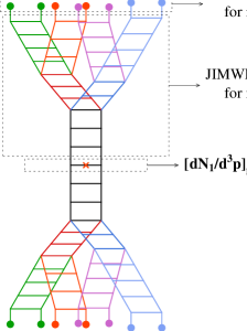
Eq. 9 is illustrated in figure
1.
Figure 1: Diagrammatic representation of the various building blocks in the
factorized formula for the inclusive single gluon spectrum. The lower part of
the figure, representing nucleus 2, is made up of identical building blocks.
As will become clear shortly, it is more convenient to express
eq. (9) in terms of color charge densities as
(11)
Here, the superscript on denotes the color charge
distribution of nucleus 1 or 2 evaluated at the rapidity .
Following a similar though slightly more involved
derivation [1], one obtains from eq. (2)
the expression
(12)
It is important to note that here we have taken , where is at an earlier
stage in the evolution of projectile and likewise, is at an earlier stage in the evolution
of projectile . This convention will be
followed for the rest of this paper.
Also, in eq. (12), is a Green’s
function of the operator ,
(13)
with the boundary condition
(14)
This Green’s function describes quantum evolution between two
specified rapidities, in the presence of strong color fields from the
projectiles. It relates the distribution of color sources at a given
rapidity with the distribution at another rapidity through the
relation
(15)
At this stage, it is important to note that the BK mean
field form of the Balitsky-JIMWLK evolution equation for the two point
Wilson line correlator (the “dipole cross-section”)
requires that the correlator of the product of traces of two pairs of
Wilson lines factorizes into the product of the correlators of traces
of pairs of Wilson lines666These Wilson lines are defined in
terms of the color charge densities through
eq. (3) projected on to a particular rapidity
,
where the ’s are the generators of the fundamental
representation of . The corresponding expression in the
adjoint representation is given in eq. (26).,
(16)
to leading order in a expansion. The averages
are performed over the color sources of a large nucleus
with the weight functional . The factorization in
eq. (16) can be achieved with Gaussian
correlations among the color sources. Note however that we need a
non-local Gaussian distribution to accommodate the quantum BK
evolution [47]. One obtains therefore777It is to be
understood that repeated color indices are summed over.
(17)
where represents the color
charge squared per unit area of nucleus 1 or nucleus 2 as seen by a
particle having rapidity . Even though in this work we will consider collisions between identical nuclei, we shall retain the
explicit notation for generality.
From eq. (2), because the functionals on the l.h.s
and the r.h.s are both Gaussians, the Green’s function
must be Gaussian as well. One obtains
(18)
where we have defined
(19)
Note that because of our choice , as defined is
always positive888 is proportional to the saturation
scale, and therefore increases as one evolves away from the
fragmentation region of a projectile..
Because the Green’s functions in eq. (2) are
expressed naturally as Gaussians in the new variables introduced in eq. (2), we
can rewrite our general expression for the double inclusive
distribution as
(20)
With the ’s from eq. (17) and the ’s from
eq. (18), the only ingredient missing in obtaining a
final expression for eq. (11) and
eq. (20) is the expression of the leading
order single inclusive spectrum in terms of the color charge densities
of the two nuclei. This expression and the subsequent simplification
of our equations for the inclusive distributions will be discussed in
the next section.
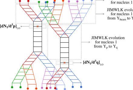
Figure 2: Diagrammatic representation of the various building blocks in the
factorized formula for the inclusive 2-gluon spectrum. As in the previous figure,
the corresponding evolution from nucleus 2 at the bottom of the figure is not
shown explicitly.
3 Gluon correlations from unintegrated gluon distributions
The leading order single particle inclusive distribution, for a fixed distribution of sources, is given by
(21)
The gauge fields are solutions of the
classical Yang-Mills equations in the forward light cone after the
nuclear collision for a fixed configuration of sources in
each of the nuclei. For Fourier modes of the color charge
densities which obey (which is
the case for ), only numerical solutions for
are
known [25, 26, 27, 28, 29, 30, 31, 32, 33].
However, for , valid for , one can perturbatively expand the gauge field in powers of
and one obtains [48, 49]
(22)
where are the structure constants and
are the Fourier transforms of the color charge
densities of the two nuclei. Here is the
well-known [50, 51] Lipatov vertex999The
components of the Lipatov four vector are , , ..
For the single inclusive distribution in
eq. (11), using
eq. (21) and eq. (22) and
the correlator
(23)
one obtains
(24)
where is the transverse area of the overlap between the two
nuclei. The unintegrated gluon
distribution can be expressed as [52, 53, 47]
(25)
where the matrices are adjoint Wilson lines evaluated in the
classical color field created by a given partonic configuration of the
nuclei or . For a nucleus moving in the direction,
(26)
Here the are the generators of the adjoint representation of
and denotes path ordering along the
axis. At large , the Wilson lines can be expanded in powers of
the sources to give, for Gaussian correlations,
(27)
Substituting this relation in eq. (24), we
obtain the well known -factorization
expression [54, 55] for the single inclusive gluon
distribution valid for :
(28)
where we denote to be the unintegrated gluon
distribution per unit of transverse area.
The corresponding expression for the double inclusive distribution is
more involved. The r.h.s of eq. (20) has the
product of two single inclusive distributions, one for a gluon with
three momentum and likewise another for a gluon with three
momentum . From eq. (21), this
corresponds to the product of four gauge fields. As for the single
inclusive case, the double inclusive gluon spectrum can be computed
numerically using lattice techniques where Yang-Mills equations are
solved to obtain the gauge fields as a function of proper time after
the collision. This computation has been carried out recently for the
Gaussian MV model [56]. Because this model does not include
the effects of small evolution, it is not ideal for the purpose of
investigating the dynamics of long range rapidity correlations.
Incorporating small evolution effects in the non-perturbative
computation is outside the scope of the present work. We will instead
consider here, as in the previous discussion of the single inclusive
distribution–see eq. (22), the perturbative limit of
, , where the gauge fields can be expanded as
bilinear products of the color sources of the two nuclei. The
dependence of the leading order double inclusive gluon spectrum on
four gauge fields, then translates, in this perturbative limit to the
product of eight color charge densities. The averages over color
sources in eq. (20) are therefore averages
over the general matrix element
where we denote by a superscript or the rapidity which
the color sources correspond to.
Further, these products of gauge fields contain bi-linear scalar
products of the Lipatov vertices. These can be
simplified [34, 57] and expressed as
The double inclusive distribution in
eq. (20), for transverse momenta , can therefore be expressed as
(31)
in terms of and
defined above.
We shall now sketch how one evaluates these quantities with further details of
the computation given in appendix A. We begin with
the evaluation of the color averages in . Because the ’s in eq. (17)
and the in eq. (2) are Gaussian weight
functionals, the relevant color source correlators are the equal rapidity correlators
(32)
and the non-equal rapidity correlators101010This follows from the
vanishing of terms odd in or .
(33)
The correlators for the dependent variables and
(see eq. (2)) are
(34)
With the relations listed, we can now evaluate eq. (LABEL:eq:F).
Simple combinatorics gives us a total of 9 possible pairwise
contractions in eq. (LABEL:eq:F). The details of these are listed in
appendix A. One of the contributions
(eq. (48)) gives the non-correlated contribution to the two
gluon inclusive distribution. Subtracting this term therefore results
in the correlated two gluon inclusive distribution
(35)
When one evaluates the other 8 terms that contribute to ,
one observes that only 4 of these give leading contributions. The
-function contributions from these terms (eqs. (49),
(50), (51), (52)) give
and . Substituting this into the expression for
in
eq. (LABEL:eq:Lipatov-product), one finds that it simplifies
considerably to read
(36)
Combining the four leading contributions from
and the
corresponding expressions from to (see eqs. (57),
(58), (59) and (60) in
appendix A), we obtain
where the ’s are unintegrated gluon distributions per unit of
transverse area and . We have used here the relation
between and the unintegrated gluon distribution given
in eq. (27). This expression is the central
result of this paper111111We note that expressions for the double
inclusive cross-section have been previously derived [58]
within the framework of Local Reggeon Field Theory [59].
At present the connection between the two frameworks is completely
unclear.. We have obtained an expression for the double inclusive
gluon distribution, valid to all orders in perturbation theory to
leading logarithmic accuracy in and for momenta , entirely in terms of the unintegrated gluon distributions of the
two nuclei evaluated at the rapidities and where . The corresponding expression for is obtained by
replacing and . We should emphasize that the notation used in eq. (LABEL:eq:double-inclusive-4) stipulates that the un-integrated gluon distributions are evaluated at rapidities .
4 Running coupling BK evolution
In the previous section, we established that the correlated two gluon
spectrum for arbitrary rapidities can be computed in terms of the
unintegrated gluon distributions of the two nuclei evaluated at these
rapidities. In this section, we shall discuss how one computes this
unintegrated gluon distribution and its evolution with . In the
next section, we shall use the results for the unintegrated gluon
distribution to evaluate eq. (LABEL:eq:double-inclusive-4) for the
correlated inclusive two gluon distribution.
In eq. (25), we defined the unintegrated gluon
distribution in a nucleus in terms of the correlator of two adjoint
Wilson lines averaged over the color charge distribution in a nucleus.
Because these averages and those of correlators of
fundamental Wilson lines are Gaussian correlators in the large
limit, one can express these correlators respectively
as [52, 60]
(38)
where is the Casimir in the adjoint representation and
is the Casimir in the fundamental
representation. The function is closely
related [47] to the variance of the non-local Gaussian
weight functional in eq. (17) and is therefore the same in
both the fundamental and adjoint cases. One can therefore, in the
large limit, simply express the correlator of two adjoint Wilson
lines as the square of the correlator of two fundamental Wilson
correlators.
The correlator of two Wilson lines in the fundamental representation
is simply related to the dipole amplitude for the scattering of a
quark-antiquark dipole (of transverse separation ) off
a nucleus as121212We assume translation invariance in the
transverse plane to set the quark transverse coordinate to zero.
(39)
where is a Wilson line in the fundamental
representation. (See our previous discussion of these in the context
of eq. (16).) Using
eq. (38), one can write the unintegrated gluon
distribution in the adjoint representation (per unit of transverse area) in eq. (25) as
(40)
We therefore need to determine the dipole amplitude and its
evolution with rapidity (=) as an input in
eq. (40) to extract the unintegrated gluon
distribution. The dipole amplitude is obtained from the
Balitsky-Kovchegov (BK) equation [38, 39], which is a
non-linear evolution equation describing both gluon emission and
multiple scattering effects in the interaction of the quark-antiquark
dipole with a nucleus in the large limit. It can be
expressed as
where . As we discussed previously, the BK
equation for the amplitude is equivalent to the corresponding JIMWLK
equation [5, 6, 7, 8, 9, 10, 11, 12]
of the Color Glass Condensate, in a mean field (large )
approximation where higher order dipole correlators are
neglected.
In the context of the BK equation, the leading order kernel
corresponds to resumming the leading terms
arising at small from all orders in perturbation theory. It is
well known however that running coupling contributions qualitatively
modify the small evolution beyond leading logarithms in and
there has been considerable recent work to include these
corrections to the BK
equation [41, 42]. The running coupling equation
describing the evolution of the dipole amplitude however takes exactly
the same form as eq. (41) with a modified evolution kernel
given by
(43)
The subscript in refers to the “Balitsky
prescription” for the evolution kernel, which corresponds to a
scheme where some particular ultra-violet finite terms are also included along with the
running coupling contributions to make the remainder numerically less
important. For a more detailed discussion, we refer the reader
to [62]. In this work, the NLO contributions not
encompassed by the kernel in eq. (43) will be
ignored. As argued previously [43], these contributions
are systematically smaller than the running coupling contribution
included here, especially at large rapidities.
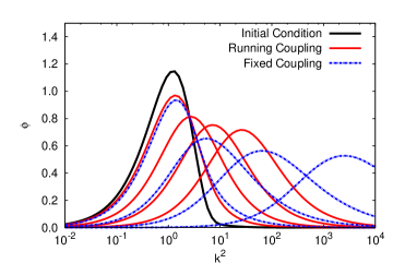
Figure 3: Unintegrated gluon distribution in the adjoint representation
at (from left curve rightwards) with the Balitsky
prescription for the kernel in eq. (43)
as well as for the fixed coupling case. The distribution is in units
of .
In fig. 3, we show results for the unintegrated gluon
distribution versus transverse momentum squared determined from the
evolution with rapidity of the dipole amplitude in the adjoint
representation (see eq. (40)) with i) the fixed
coupling BK kernel, and ii) with the Balitsky prescription for the
kernel in eq. (43)). As we will describe below,
the initial conditions for the latter figure are constrained by
fixed target e+A data. We note that the evolution of the unintegrated
gluon distribution with Balitsky’s prescription for the running
coupling effects is significantly slower than the evolution with a
fixed coupling constant.
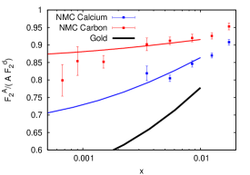
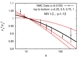
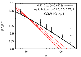
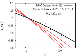
Figure 4: The and dependence of the normalized ratio of
structure functions in nuclei. The curves in the left figure
includes effects due to the small evolution of the dipole
cross-section described by the BK evolution with the modified kernel
in eq. (43). The curve in the right
figure is sensitive to the dependence of the initial condition
alone because it is evaluated at relatively large . Details
regarding the parameters of the initial condition are discussed in
appendix B. The data are from the NMC
collaboration [63]. Figure 5: The dependence of the ratio of structure functions given
by data from the NMC collaboration [64]. The corresponding
curves for other initial conditions are in appendix B.
The BK equation with the modified kernel in
eq. (43) was first applied in
Refs. [43, 44] to a phenomenological study of the
HERA data on the proton structure function . Two sets of initial
conditions for the dipole amplitude at the initial rapidity
were used–the GBW [65] and MV initial
conditions [2, 3, 4]–and their parameters
determined from fits to the HERA data. To constrain the initial
conditions for nuclei and therefore extract the nuclear unintegrated
gluon distribution, we performed a fit to the available NMC data on
the nuclear structure function . The details of the
fit and the results are described in detail in appendix B. We show
here in figs. 4 and 5 representative
plots of fits to , and dependence of the fixed target e+A
data. Good fits to the available data are obtained for both sets of
initial conditions for particular parameters. With the initial
conditions for the BK equation
fixed by the NMC data, we shall now use the corresponding unintegrated
gluon distribution to study long range rapidity correlations in the
Glasma.
5 Results for long range rapidity correlations in the Glasma
In this section, we will make use our result in
eq. (LABEL:eq:double-inclusive-4) for the double inclusive gluon
distribution to compute long range rapidity correlations in A+A
collisions at RHIC and the LHC. The essential ingredient in
eq. (LABEL:eq:double-inclusive-4) is the unintegrated gluon
distribution which, as shown in eq. (40), is simply
related to the dipole scattering amplitude. The evolution of the
dipole scattering amplitude with rapidity (or ) is described by the
BK evolution equation given in eq. (41), with the modified kernel
given in eq. (43). The rapidity dependence of the
double inclusive gluon spectrum therefore provides a sensitive test of
high energy QCD evolution.
Equation (LABEL:eq:double-inclusive-4) is derived
in the leading approximation, where all transverse momenta
are assumed to be parametrically of the same order
as . In this approximation
the -values at which the unintegrated gluon distributions are evaluated
are not exactly determined, as long as ,
where is the appropriate rapidity of the produced gluon ( or )
and the sign depends on the nucleus (1 or 2) considered.
We define the longitudinal momentum fractions of the
produced gluons with respect to nucleus 1 or 2 (denoted by subscripts)
(44)
In the above expression, and are the transverse momenta
of the produced gluons. The unintegrated gluon distributions
with momentum argument and in
eq. (LABEL:eq:double-inclusive-4) are evaluated at these values of
the momentum fraction. For the unintegrated distribution
with momentum argument we replace the transverse
momentum in eq. (44) by to make
our evaluation of eq. (LABEL:eq:double-inclusive-4) manifestly
symmetric in and 131313Another option would be to replace the momentum in eq. (44) by . We have tried this and found our results to be insensitive to the choice of scale.. Our derivation in Sec. 3
makes it clear that the term
with in eq. (LABEL:eq:double-inclusive-4) should be evaluated
at a rapidity scale that is the earlier of the two rapidity scales
and in the evolution of the corresponding nucleus. This
prescription guarantees that the same is true when the scale is parametrized
in terms of instead of rapidity.
The solution of the BK equation is reliable when the gluon density is
large. The initial condition for the evolution is typically set at . For larger values of , one expects the BK description
to break down; we use instead a phenomenological extrapolation (used
previously in [66, 47]) for the unintegrated gluon
distribution which has the form
(45)
where and the parameter . This extrapolation to
large is unreliable and depends on physics which is not amenable
to the renormalization group approach advocated here. However, in
experiments with finite kinematic reach, it is inevitable that one is
sensitive to the non-perturbative physics at large in some
kinematic range. For example, from the kinematic expressions in
eq. (44), the unintegrated gluon distribution of gluons having
GeV at RHIC energies of GeV/nucleon will
begin to be sensitive to the large extrapolation of the
distribution at units in rapidity. At the LHC
energy, the range in rapidity where we avoid this sensitivity is much
greater. At TeV, the same gluon does not probe the
large extrapolation of the unintegrated gluon distribution until
With these caveats in mind, we shall now examine the two gluon
inclusive distributions in A+A collisions both at RHIC
( GeV)
and at the LHC ( TeV). The beam rapidities for
these energies are and for
RHIC and LHC respectively. We will first consider RHIC collisions and
compare our results to recently measured long range rapidity
correlations in the near-side ridge by the PHOBOS collaboration. The
experimental quantity of interest is , where the trigger particle
consists of all particles having GeV and an
acceptance in rapidity in the range . The particles associated with this trigger have momenta larger
than 4 (35) MeV at a rapidity of 3 (0). In performing the projection in the experiment, the near side yield is integrated
over . Hence in computing the
per-trigger yield, we should in principle also integrate our two
particle correlation over the PHOBOS acceptance. We will
instead perform a more qualitative comparison here by computing
instead our two particle correlation at representative values of the
trigger and associated particle momenta and multiplying the result by
the phase space volume corresponding to the PHOBOS acceptance.
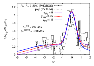
Figure 6: Comparison of our results for long range rapidity
correlations to data from the PHOBOS collaboration [19].
The curves shown are obtained by adding our result (expressed by
eq. (46) for long range rapidity correlations in the PHOBOS acceptance to the short range jet correlation in p+p collisions
obtained using PYTHIA.
For the trigger particle we take GeV at and units in rapidity. We assume the
associated particle has mean MeV. For all cases, we
compute the yield at . Then, in terms of our
expression for the two particle cumulant, the required quantity can be
written as
(46)
where is the two particle cumulant given by
eq. (LABEL:eq:double-inclusive-4). In the above expression, the phase
space volume corresponding to the trigger particle cancels out; we are
left with an overall factor from the associated particle’s phase space
volume, , which we estimate to be
GeV2. We arrive at this
estimate by performing the angular integration over
times the integration over the
acceptance. Other than , the only
additional parameter in our expression is which we
take to be . With these stated values of
and , our overall normalization is now
fixed. The function comes from the collimation
of the Glasma flux tubes due to radial flow as discussed in
Ref. [34]. At , this can be expressed
as
(47)
where is the radial flow velocity.
To take into account the short range correlation from fragmentation
not included in our formalism we add to eq. (46)
the short range jet correlation resulting from PYTHIA.
The result is compared to the PHOBOS experimental
data [19] in fig. 6.
One can see that the agreement with data is quite good. In principle the collimation from radial flow through eq. (47) can be a function of rapidity. We have estimated this effect by assuming that the space-time and momentum space rapidity are strongly correlated.
From fits to BRAHMS data
[67, 68, 69] on the inclusive hadron spectrum, we
estimate the dependence of the flow velocity to be . When including this rapidity dependent flow through eq. (47), the effect is so small that it would not result in a
visible change to the curves plotted in figure 6.
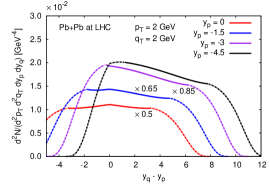
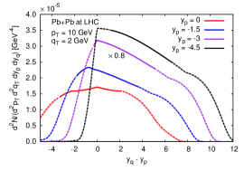
Figure 7: The predicted two particle correlation spectrum as a function
of the rapidity difference between the two gluons. The figure on the
left corresponds to the case where the transverse momenta of the two
gluons are equal and are GeV; the figure on the
right depicts the case where GeV and GeV.
The different plots reflect different trigger rapidities. Solid
parts of each curve correspond to in both nuclei; the
dashed parts are sensitive to in at least one of the
nuclei. We have rescaled some curves, by the given factors, for clarity.
At RHIC energies, the range in rapidity where the results are
sensitive to small physics exclusively is quite limited. At the
LHC, this range is much larger and the effects of QCD evolution on
long range rapidity correlations is more transparent. In
fig. 7, we show results for the two particle cumulant
as a function of the rapidity difference between
the two gluons. In the figure on the left, the correlation is plotted
for GeV; the right figure corresponds to the
asymmetric case of GeV and GeV. For both
scenarios, we show the evolution in rapidity of the two particle
correlation at different trigger rapidities . The solid part of
each curve corresponds to the kinematic range where only
values in each of the nuclear wavefunctions are being probed. In
contrast, the dashed part of each curve denotes the kinematic range
which is sensitive to for at least one of the nuclei; in
this regime, the results are more sensitive to the form chosen for the
large extrapolation than to the high energy QCD evolution equations at
small . Because of the large kinematic reach of the LHC, we
observe in fig. 7 that we have a region contributing to the
double inclusive rapidity spectrum, of nearly units in the
rapidity difference of the two gluons, which is sensitive only to the
small evolution in the nuclear wavefunctions. The shape and
magnitude of these correlations will therefore give us unique insight
into the evolution of multi-parton correlations in high energy QCD.
6 Summary
In Ref. [1], a general formula
(eq. (12)) was derived for double inclusive
gluon production in the Glasma at arbitrary rapidity separations. In
this paper, we showed that this formula reduces to a compact
expression, eq. (LABEL:eq:double-inclusive-4), in terms of the
unintegrated gluon distributions in the two nuclei. This
simplification holds when , and when the
mean field Balitsky-Kovchegov (BK) framework — valid in the
large limit — is used to describe the high energy evolution
of the nuclei. The unintegrated gluon distributions at small are
simply related to the dipole foward amplitude, which in turn satisfies
the BK equation. Solving the running coupling form of the
BK equation, with initial conditions determined from fits to fixed
target e+A data, we computed the double inclusive spectrum at RHIC and
LHC energies. In the case of the former, we obtained a good agreement
with the PHOBOS data, albeit the kinematic region where small
partons are probed in both nuclei is rather small. In the latter case,
we showed that there is a wide kinematic window for rapidity
correlations at the LHC. Our results therefore open a new window into
the study of the high energy evolution of multiparton correlations in nuclear
wavefunctions.
Acknowledgements
We thank Javier Albacete, Adrian Dumitru, Anna Stasto and Kirill Tuchin for very
useful discussions. We are especially grateful to Gregory Soyez for
his co-ordinate space BK code. K.D. and R.V.’s research is supported
by the US Department of Energy under DOE Contract No.
DE-AC02-98CH10886. T.L. is supported by the Academy of Finland,
project 126604. F.G. is supported in part by Agence Nationale de la
Recherche via the program ANR-06-BLAN-0285-01.
Appendix A Evaluation of eq. (LABEL:eq:F)
In this appendix, we work out some of the details of the derivation of
the double inclusive spectrum. In particular, eq. (LABEL:eq:F) is
expressed as the product of eight color charge densities. For a
non-local Gaussian distribution of these sources, one has nine
possible pairings of color source densities. These are evaluated
explicitly below.
(48)
(49)
(50)
(51)
(52)
(53)
(54)
(55)
and
(56)
The classification of these contributions was examined previously in
[34] in the framework of the MV model. The analysis is
identical here. The expression is trivial as it
cancels the square of the single particle distribution. Let us look at
the -functions in . These yield a
local -contribution that we shall neglect here
as in Ref. [34]. Similarly,
expressions are sub-dominant141414We note that there is an order one contribution coming from when the relative angle between is . In the limit where these contributions will be washed out by re-scattering in the same manner as the -function contributions coming from , and thereby not alter our result. We thank Kirill Tuchin for pointing out this subtlety to us.. The leading
terms are therefore . If we plug these
back into eq. (31), we obtain the following
four contributions to the two gluon spectrum
(57)
where
,
(58)
where ,
(59)
where
,
and finally
(60)
where . Using
eq. (27), we can express
as eq. (LABEL:eq:double-inclusive-4).
Appendix B Initial conditions for BK evolution
The initial conditions for BK evolution of protons and nuclei are
obtained by comparing results for the dipole cross-section to deep
inelastic scattering data. The inclusive structure function is
given by
(61)
where is the virtual photon-nucleus cross section for
transverse and longitudinal polarizations of the virtual photon. These in turn are given by
(62)
where is the dipole-nucleus scattering amplitude. We assume here that the dependence can be factorized as
(63)
The virtual photon-nucleus cross section can then be expressed as
(64)
where
(65)
Initial condition for protons
The initial condition for protons was determined from a global fit of
data in the work of [43]. Two different models for
the initial condition were used in that work. The first is the GBW
model
(66)
and the other is the MV model
(67)
The fit parameters obtained in [43] are summarized in the table
1.
I.C.
(fm2)
(GeV2)
GBW
3.159
0.24
5.3
NA
MV
3.277
0.15
6.5
1.13
Table 1: Parameters for the initial condition of the
proton dipole cross section obtained in [43].
Initial condition for nuclei
We shall now consider the initial conditions for nuclei using the same
model as the initial conditions for protons. We do not attempt to
perform a global fit since the data for DIS off nuclei are not nearly
of the same quality. We use a model where the initial saturation
scale scales linearly with ,
(68)
where is a constant to be determined from the data.
In order to constrain the initial condition, we begin by looking at
the New Muon Collaboration’s (NMC) data [64] for
as a function of at which is close to
our . In this case, there is no BK evolution, and we have a
direct comparison of the nuclei’s initial condition with the data. In
computing we will need a model for how the cross section
scales with . We take . Figure 8 shows the NMC data as a
function of for the GBW initial condition for four different
values of (left) and the MV model initial condition having
anomalous dimension (right). It is clear that in order to
be consistent with the data we must take . The nuclear
saturation scale given by eq. (68) is too small to be
consistent with measurements by other groups.
Figure 8: DIS fixed target e+A data on the ratio of structure functions
as a function of for fixed . The plots correspond to
(right) MV model initial condition having and (left) GBW
initial condition.
In fig. 5, we show the NMC data on the ratio of structure
functions as a function of now using the MV initial condition with
anomalous dimension . We find that for this
fits the data rather well. Based on the above results, for nuclei
we will use the MV model and take and . Therefore we have and
(GeV)2 for C, Ca, Sn and Au respectively. Note that these
values of the saturation scale are for quarks in the fundamental
representation. For gluons in the adjoint representation, the
corresponding saturation scale is
(69)
For gold nuclei this yields GeV2 at ,
in fairly close agreement to the value of GeV2 obtained in
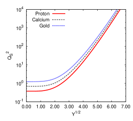
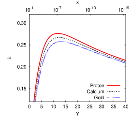
[18, 70]. Finally, we plot in fig. 9 (left)
the saturation scale in the running
coupling case as a function of for the proton, calcium and
gold nuclei. The behavior at small is sensitive to the
initial conditions of each of these nuclei; however, at large
(small ) the curves of the three nuclear approach the
same slope, as one expects asymptotically for the behavior of
when running coupling effects are accounted for (see also
[71]). The same trend can be observed by plotting
(see fig. 9 right)
, the parameter that sets the rate at which the
dipole amplitudes evolve with rapidity. These results confirm the
universal behavior at large predicted in Ref. [72].
Figure 9: Left: The saturation scale as a function of the square
root of the rapidity for protons, calcium and gold nuclei.
Note that the slopes of the three curves approach the same value at
large . Right: as a function of
approaches a universal value at large .
References
[1]
F. Gelis, T. Lappi, R. Venugopalan, Phys. Rev. D79, 094017
(2009).
[2]
L.D. McLerran, R. Venugopalan, Phys. Rev. D49, 2233 (1994).
[3]
L.D. McLerran, R. Venugopalan, Phys. Rev. D49, 3352 (1994).
[4]
L.D. McLerran, R. Venugopalan, Phys. Rev. D50, 2225 (1994).
[5]
J. Jalilian-Marian, A. Kovner, L.D. McLerran, H. Weigert, Phys. Rev. D55, 5414 (1997).
[6]
J. Jalilian-Marian, A. Kovner, A. Leonidov, H. Weigert, Nucl. Phys. B504, 415 (1997).
[7]
J. Jalilian-Marian, A. Kovner, A. Leonidov, H. Weigert, Phys. Rev. D59, 014014 (1999).
[8]
J. Jalilian-Marian, A. Kovner, A. Leonidov, H. Weigert, Phys. Rev. D59, 034007 (1999).
[9]
J. Jalilian-Marian, A. Kovner, A. Leonidov, H. Weigert, Erratum. Phys. Rev.
D59, 099903 (1999).
[10]
E. Iancu, A. Leonidov, L.D. McLerran, Nucl. Phys. A692, 583
(2001).
[11]
E. Iancu, A. Leonidov, L.D. McLerran, Phys. Lett. B510, 133
(2001).
[12]
E. Ferreiro, E. Iancu, A. Leonidov, L.D. McLerran, Nucl. Phys. A703, 489 (2002).
[13]
T. Lappi, L.D. McLerran, Nucl. Phys. A772, 200 (2006).
[14]
F. Gelis, R. Venugopalan, Acta Phys. Polon. B37, 3253 (2006).
[15]
F. Gelis, T. Lappi, R. Venugopalan, Int. J. Mod. Phys. E 16, 2595
(2007).