Massive Neutrinos and Magnetic Fields in the Early Universe
Abstract
Primordial magnetic fields and massive neutrinos can leave an interesting signal in the CMB temperature and polarization. We perform a systematic analysis of general perturbations in the radiation-dominated universe, accounting for any primordial magnetic field and including leading-order effects of the neutrino mass. We show that massive neutrinos qualitatively change the large-scale perturbations sourced by magnetic fields, but that the effect is much smaller than previously claimed. We calculate the CMB power spectra sourced by inhomogeneous primordial magnetic fields, from before and after neutrino decoupling, including scalar, vector and tensor modes, and consistently modelling the correlation between the density and anisotropic stress sources. In an appendix we present general series solutions for the possible regular primordial perturbations.
I Introduction
The origin of the G magnetic fields observed in galaxies and clusters poses something of a problem for contemporary astrophysics Kulsrud and Zweibel (2008). Recent observations of galaxies at redshift — seem to show the fields were of comparable strength when the Universe was much younger, disfavouring a large dynamo amplification from tiny G seed fields Wolfe et al. (2008); Bernet et al. (2008). Tentative observations of magnetic fields in elliptical galaxies, and a detection in a dwarf galaxy, also disfavour several dynamo mechanisms because they have little coherent rotation (see Widrow (2002) and references within). There is also some evidence for G fields coherent on megaparsec scales Lee et al. (2009). It may be possible to explain these observations in terms of astrophysically generated seed fields. Another interesting possibility is a primordial seed field. A primordial G (comoving) field could lead to the observed galactic fields via adiabatic contraction alone, and might leave an interesting observable signature in the CMB. In this paper we revisit the calculation of the CMB power spectrum from primordial inhomogeneous magnetic fields and work towards robust theoretical predictions that can be used to test the primordial field scenario with CMB data. Since primordial magnetic fields are expected to be exponentially small in most early-universe models, any detection would be a clear signature of something very interesting.
If a primordial inhomogeneous magnetic field is present it sources scalar, vector and tensor modes, giving rise to a signal in the CMB temperature as well as E and B-mode polarization. Previous calculations have indicated that G fields (comoving) are detectable Yamazaki et al. (2006); Paoletti et al. (2008), but have been incomplete in several respects. One complication is that the anisotropic stress due to the magnetic fields becomes compensated by the neutrino anisotropic stress Lewis (2004), significantly reducing the perturbations sourced on large scales after neutrino decoupling. Recent work by Kojima et al. Kojima et al. (2008) has claimed that the presence of massive neutrinos leads to a significant change in this compensation mechanism, giving rise to a dramatic enhancement of up to eight orders of magnitude on the large-scale E-mode polarization power spectrum. For interesting neutrino masses this would, if true, be a clear signal of primordial magnetic fields. Clearly this claim merits further investigation, though we shall ultimately show that the effect, though interesting, is much smaller than previously claimed.
In the early universe the massive neutrinos are expected to be relativistic, with the most massive eigenstate only becoming non-relativistic around recombination or later Lesgourgues and Pastor (2006). We perform a systematic analysis of the primordial perturbations to lowest order in the mass, generalizing previous results for the general primordial perturbation to the realistic case where one or more of the neutrinos is massive. This also allows us to calculate the series solutions consistently in the presence of magnetic fields, and see the leading corrections due to the neutrino mass effect. We also discuss the tight coupling approximation, which is useful after the modes come inside the horizon but before Thomson scattering becomes ineffective.
The calculation of the CMB power spectrum from primordial magnetic fields is further complicated because the scalar, vector and tensor sources are all quadratic in the underlying magnetic field, and the scalar modes have more than one source term. These sources are correlated, so we show how to calculate the various source power spectra and correlations from the power spectrum of the magnetic field, and how to use these for a numerical calculation.
In this work we address the effects of magnetic fields in sourcing primary anisotropies in the CMB, however, magnetic fields present after recombination also have an observational effect on the polarisation by inducing Faraday rotation Kosowsky et al. (2005); Scóccola et al. (2004). Such rotation converts E-mode polarisation into B-modes with a strong dependence on the frequency of the radiation but it is small at the usual frequencies for CMB observation, and we will neglect it in our analysis.
Throughout this work we use a 3+1 splitting of General Relativity, working with a gauge invariant linear perturbation theory similar to that of Bardeen Bardeen (1980) and Durrer Durrer and Straumann (1988); Durrer (1994). Our choice of gauge invariant variables is chosen as a close analogy to the Conformal Newtonian Gauge (CNG). We use a metric
| (1) |
where we can further decompose and into their scalar, vector and tensor contributions. Our decompositions are performed in the same manner as Ref. Hu and White (1997). In -space the decomposition for the rank-1 and rank-2 three-tensors are written as (using and as examples)
| (2) |
where the harmonic functions give the form of each perturbation type for a specific mode, with giving scalar perturbations, and , , vector and tensor respectively. In the above it should be understood that we implicitly sum over the two vector and two tensor modes, for example
| (3) |
whilst a quantity like appearing on its own can stand for either or consistent with the context. The scalar harmonic functions are
| (4) | ||||
The vector harmonics are
| (5) |
where we decompose our vectors with the helicity basis
| (6) |
with and being unit vectors orthogonal to . Note that , whilst . From this we can see that . For the tensors we make the further definition of . Using this, the sole tensor harmonic is
| (7) |
For reference the self contraction of this is . As we would expect, quantities of different types are always orthogonal, for example .
Generally we will drop the superscript on scalar perturbations like , in favour of simply .
As a further illustration, let us examine the perturbations to the energy-momentum tensor . In the Conformal Newtonian Gauge, the gauge invariant quantities we use are exactly equivalent to perturbations of the Energy-Momentum tensor. The density , velocity , pressure , and anisotropic stress perturbations are defined by
| (8) | ||||
| (9) | ||||
| (10) |
where and are the density and pressure respectively. As above we will further decompose the three-vector and tensor quantities into the different perturbation types. The velocity three-vector decomposes as
| (11) |
where the vorticity is the vector-type velocity. The traceless anisotropic stress tensor becomes
| (12) |
Generally we will rewrite the pressure perturbation in terms of an entropy type perturbation and the density
| (13) |
Although we will not explicitly demonstrate it, is gauge-invariant. Above we have used and , defined as and the sound speed .
We will restrict ourselves to a flat geometry throughout this work.
II Neutrino Perturbations
II.1 Kinetic Theory
To describe the behaviour of neutrinos in the early universe, we must turn to the full machinery of the Boltzmann equation. We start with the phase space distribution of the particle density on a spatial hypersurface, defined by
| (14) |
where is the canonical 3-momentum, the spatial part of the covariant 4-momentum . The primary quantity we will require is the energy-momentum tensor which is determined from the distribution function by
| (15) |
Following the convention in the literature Durrer (1994); Ma and Bertschinger (1995) we will re-express the distribution function in terms of quantities in the frame of a comoving observer. We use the locally Minkowski tetrad satisfying . In terms of the co-ordinate basis, and where we have avoided fixing a gauge
| (16a) | ||||
with containing the trace-free scalar, vector and tensor contributions. This allows us to write the momentum in terms of quantities measured in the comoving tetrad , where is the observed energy and the momentum in that frame. Applying Hamilton’s equations to the system implies that the conjugate momenta will remain constant in a purely FRW universe. This means the proper 4-momenta will decay away with . In order to remove this redshifting of the energy and momenta we will write them in terms of the scaled quantities and defined by
| (17) |
where is the unit vector in the direction of the momentum. Both and are constant on the background by definition. By considering we find a slightly modified energy momentum relation
| (18) |
Prior to their decoupling, neutrinos are in approximate thermal equilibrium with the rest of the Universe. Considering only the unperturbed case for the moment, the phase-space distribution function of the neutrinos will be Fermi-Dirac at a universal temperature. We expect this distribution to be isotropic and homogenous, and thus only be a function of the momentum magnitude (in the guise of the comoving energy) and the time (by virtue of the temperature). Therefore it takes the form
| (19) |
where the neutrino energy measured by a comoving observer is . As the temperature decreases with , the combination is constant, depending on , the temperature today.
At neutrino decoupling, this distribution becomes frozen in. The neutrino mass is insignificant compared to any thermal energy, so its contribution can be neglected in the distribution function. This allows us to set (within the distribution only), leaving the unperturbed function as
| (20) |
We will define the first order perturbations to the distribution by
| (21) |
with containing the scalar, vector and tensor contributions. This quantity is gauge dependent; later we will form a gauge invariant equivalent.
We want to rewrite the integral (15) in terms of our comoving quantities, retaining terms up to first order. Firstly, the term forms a co-ordinate invariant measure for the integration, and can be re-written in terms of the comoving quantities
| (22) |
This removes the metric perturbations contained within the integration measure. Re-expressing the generates a plethora of terms, including terms first-order in the metric perturbations. However these terms all depend upon a single power of the momentum direction and couple only with the isotropic distribution ; they are thus eliminated by their symmetry. The remaining terms are simply
| (23) |
Decomposing into distinct components this leaves us with
| (24) | ||||
valid in all gauges up to first order.
The evolution of the distribution function is governed by the collisionless Boltzmann (or Vlasov) equation, which simply expresses that, without collisions, the number of particles is conserved along a trajectory in phase space
| (25) |
In order to address the evolution of the perturbations to the distribution function, we need to separate this out into equations for the background, and the separate perturbation types. We address this in subsequent sections.
II.2 Background Quantities
At zeroth order the collisionless Boltzmann equation simply shows that the distribution remains constant, that is, is independent of time. At this order the energy-momentum tensor can be described fully in terms of density and the pressure. The density is given by
| (26) |
With a non-zero neutrino mass the pressure is no longer simply related to the density. It’s instead
| (27) |
As we would expect, the equation of state is still defined by the ratio of these two quantities, yielding a mass dependent .
II.3 Scalar Perturbations
Initially we will just address scalar perturbations to the distribution function , considering vectors and tensors later on.
We will perform a harmonic expansion of all our quantities. In flat-space this is just the Fourier transform. The Boltzmann equation (25) can be expanded at first order including all the (non-gauge fixed) metric perturbations Durrer and Straumann (1988) giving
| (28) |
where and the dot is the derivative with respect to conformal time . To move to a gauge-invariant formalism we follow Durrer and Straumann Durrer and Straumann (1988) and define a new gauge-invariant distribution perturbation
| (29) |
where is the shear on spatial hypersurfaces , and is the conformal Hubble parameter. This differs from Durrer’s definition in that we have chosen our definition to coincide with the CNG result (added terms vanish in a zero-shear gauge). For comparison Durrer’s invariant perturbation and our definition are linked via
| (30) |
Instead of the scalar metric perturbations we will use the gauge-invariant Bardeen potentials
| (31) | ||||
| (32) | ||||
The potential should not be confused with the distribution perturbation . Usually the context will make this clear. In the above, is the 3-Ricci scalar
| (33) |
Written in terms of gauge-invariant quantities, the Boltzmann equation becomes
| (34) |
As mentioned, our choice of gauge invariant variables is designed such that this is equivalent to the CNG version.
The dependence on the momentum direction within the Boltzmann equation makes a direct solution tricky. We take the standard approach and expand out into an angular basis. Whilst for scalar perturbations it suffices to expand in the Legendre polynomials , for vector and tensor perturbations it is much more convenient to use a method similar to Ref. Hu and White (1997), where we expand out into spherical harmonics . Under this expansion, the different types of perturbations are separated by their value, with scalar (), vector () and tensor () modes all evolving separately in the usual manner. Expanding out the entire distribution perturbation
| (35) |
we can relate the momentum integrals of the multipole moments to the standard gauge invariant perturbations
| (36) | ||||
II.4 Thermal Perturbations
The most natural perturbation that could be set up is from a purely thermal distribution, where we perturb the neutrinos by having a position and direction dependent change to the temperature. To take this into account let us re-write our distribution perturbation in a slightly different manner. The total distribution
| (37) | ||||
For generality we leave a function of . For a pure temperature perturbation it must be temperature independent. Relating this to our previous gauge invariant perturbation we find that
| (38) |
and from this construct a temperature-like gauge-invariant perturbation
| (39) |
such that . Substitution into the Boltzmann equation (34) produces
| (40) |
When or , and the Boltzmann equation becomes momentum independent; the perturbation remains purely thermal. However even perturbations which start in a purely thermal state evolve away from it as the mass becomes important. For this reason we must keep a function of , though we will restrict ourselves to purely thermal initial conditions.
III Mass Expansion
To treat massive neutrinos in the early Universe, when the mass is small in comparison to the typical momentum (approximately ), we will expand the system to first order in the neutrino mass squared. This will allow us to directly tackle the integrated distribution function, making it possible to find initial conditions up to this order in the neutrino mass. For a more general approach see Lewis and Challinor (2002).
In both the integrals for the energy-momentum tensor and the Boltzmann equation itself the mass dependence comes in from factors of or its inverse. Expanding this out gives (with a minus for the inverse). For the background quantities performing this expansion gives
| (41) | ||||
where is the density for massless neutrinos, and the scaled mass , with the factor being defined via
| (42) |
which is essentially the momentum averaged inverse square momentum. This depends only on the background distribution, and is time independent. Thus we factor it into the new dimensionless mass . In terms of background quantities
| (43) |
As with the density we expand up to for the background pressure and the equation of state giving the form
| (44) |
The perturbed quantities are slightly more tricky. For example taking and expanding out in mass gives,
| (45) |
with a similar pattern for the other perturbations. Schematically we have two types of terms we need to integrate; and . For a moment let us consider what happens to these integrals for thermal perturbations in the case of massless neutrinos
| (46) |
and similarly the second integral equates to
| (47) |
From this we can make the connection that, at zeroth order in the mass expansion, the second integral is linked to the first via
| (48) |
and as the second integral appears at first order in in the mass expansion, we can use this relation to simplify the expression for above, giving
| (49) |
This happens similarly with the other perturbed quantities, and allows us to follow the convention of forming a momentum integrated function
| (50) |
As with the distribution perturbation, we will expand into spherical harmonics
| (51) |
Each moment takes the same form as the integrated of (III) with the being replaced by .
These lead to a succinct form for the perturbations
| (52) |
to order . Similarly,
| (53) |
All that we need to do to have a working prescription for calculating the massive neutrino evolution is to turn the Boltzmann equation into a hierarchy for solving for the . First we take the Boltzmann equation and expand to first order in , then integrate it over and divide by the same quantity to produce an equation for the evolution of . We employ the same trick as above (in Eq. (48)) to turn the quantities into terms in . This results in
| (54) |
We then substitute a spherical harmonic expansion for , and using the identity that
| (55) |
we obtain the hierarchies for . Separating these out into coupled equations for each gives three distinct cases. For the monopole ()
| (56a) | |||
| For the dipole () | |||
| (56b) | |||
| Finally for the quadrupole and higher moments () | |||
| (56c) | |||
As should be expected sending takes everything to the well known massless case.
Taking this mass expansion to higher order becomes more difficult: Taylor expanding the background quantities inside the integral produces divergent integrals at order and above. We show how to do the higher-order expansion in Appendix A; this shows that the leading-order mass expansions are correct to .
IV Vector Perturbations
To consider vector perturbations we proceed down a similar line to the scalar perturbations. Though not entirely free of gauge issues, many of the complexities will disappear. Firstly, whilst there are two vector-type metric perturbations and , we have one degree of gauge freedom, and so only one perturbation can be relevant. As before, rather than fixing a gauge we form one gauge-invariant variable. For vector perturbations, the shear-like perturbation is gauge-invariant and we use this as our metric variable.
The vector contribution to the distribution function is itself gauge-invariant, (see Durrer (1994)), and thus the Boltzmann equation governing it is
| (57) |
There are two contributions to the energy-momentum tensor: the velocity, , which is gauge dependent, and the anisotropic stress which is gauge-invariant. As a gauge-invariant velocity, we use the neutrino vorticity which is conveniently related to the distribution perturbation. The two neutrino perturbations are therefore
| (58) |
Performing the same momentum integration as for the scalars (with the same restriction to thermal modes), we find an equation governing the momentum-integrated
| (59) |
where we have used that . Inserting the spherical harmonic expansion, and using the identity (55), the moments of the Boltzmann equation are for
| (60) |
for
| (61) |
and for
| (62) |
Finally we need to rewrite both and in terms of the integrated functions. These are nearly identical to the scalar equivalents, only with different coefficients
| (63) |
V Tensor Modes
As is well known, tensor perturbations are manifestly gauge invariant and so we need not concern ourselves with any gauge issues. Other than that we follow the same track as for the scalar perturbations. The Boltzmann equation for tensor modes takes on the form
| (64) |
We then momentum integrate the equation to produce a single equation in terms of the . Again we have restricted ourselves to initially thermal perturbations, giving
| (65) |
Using the helicity basis, the quantity is simply written in terms of spherical harmonics as
| (66) |
To finish off, we need to rewrite the Boltzmann equation (65) with a spherical harmonic decomposition. There are no relevant contributions from the , and terms in the sum. For we have
| (67) |
and for we require
| (68) |
The only tensor contribution to the energy momentum tensor comes from the anisotropic stress . This is easily expressed in terms of the expanded with
| (69) |
VI Evolution Equations
The behaviour of the early Universe is accurately described by linear perturbation theory, reducing to a system of coupled linear differential equations. We have discussed the perturbation equations for the neutrinos in previous sections. Here we briefly describe the remaining equations for the evolution of the metric potentials and the other matter species.
The splitting of the Einstein equation decomposes into sets of equations for each of the scalar, vector and tensor contributions. For the scalar perturbations we have four equations generated by the splittings. There are two equations formed by the and components
| (70a) | ||||
| (70b) | ||||
| where the first is the equivalent of the classical Poisson equation. The spatial part () splits into two further equations from the trace and traceless parts. The equation from the trace is | ||||
| (70c) | ||||
| where is the perturbation to the entropy of the system, and is the total sound speed of all the matter species. The final equation is from the traceless part | ||||
| (70d) | ||||
There are two vector equations, one from the part, and the second from the vector contribution to the components:
| (71a) | ||||
| (71b) | ||||
There is a single equation for the tensor modes
| (72) |
The matter evolution equations are well known and are most generally derived from the Boltzmann equation, here we will just give the results. We consider the standard three matter species beyond neutrinos: baryons, photons and cold dark matter, giving their perturbations in terms of , and as before.
The matter species have essentially no velocity dispersion, the anisotropic stress and higher momentum moments are all zero. Hence they contribute only to scalar and vector modes and can be described entirely in terms of , and . Simplest is dark matter as it has no interactions. For the scalars
| (73a) | ||||
| (73b) | ||||
| and for the vectors | ||||
| (73c) | ||||
We can see that any vector solution for CDM must be decaying, and so we will neglect it.
The baryons couple to the photons via Thomson scattering, but also interact with any magnetic field via the Lorentz force giving an extra source term
| (74a) | ||||
| (74b) | ||||
| where the baryon sound speed is . The two quantities and are the magnetic equivalents of the density and anisotropic stress perturbations. We make a thorough definition in the next section. The vector equation is | ||||
| (74c) | ||||
where and is the timescale for Thomson scattering, the inverse of the opacity, . As with CDM there are no tensor perturbations to the baryon distribution.
Describing the photon perturbations requires the full mechanics of the Boltzmann distribution. Constructing the gauge invariant perturbation equations is done in the same manner as for the neutrinos, with the distinction that they are are massless bosons, and interact with the baryons via Thomson scattering (see Durrer (1994); Hu and White (1997)). The full calculation requires a consistent treatment of polarization; we do not repeat this here, see e.g. Ref. Hu and White (1997) for the details. The photon hierarchy is concisely written as
| (75) |
the source terms describe the interactions with the gravitational potentials and other matter species. The non-zero terms are for the scalars
| (76a) | ||||||
| for the vectors | ||||||
| (76b) | ||||||
| and for the tensors | ||||||
| (76c) | ||||||
where is the anisotropic Thomson source and contains the coupling to the polarisation
| (77) |
In terms of the photon multipole moments the usual matter sources are
| (78) | ||||||||
VI.1 Regular initial conditions
We use the full system of perturbation equations to calculate initial series solutions for modes well outside the horizon in the early radiation-dominated epoch, after neutrino decoupling but well before recombination. These are needed to provide the correct initial conditions for Boltzmann codes such as Camb Lewis et al. (2000) and Cmbfast Zaldarriaga and Seljak (2000). We have calculated the complete set of all known regular modes for the standard matter species (dark matter, baryons, photons and neutrinos) for the scalar, vector and tensor type perturbations. We have also included all the compensated magnetic modes for three perturbations types. By using our expanded neutrino equations (see Section III) we can include neutrinos of non-negligible mass, with solutions accurate to order . Thus our solutions include both massless neutrinos and a number of degenerate massive species.
We make several standard approximations, firstly we assume we are in the regime of tight coupling between photons and baryons where Thomson scattering prevents slippage between the fluids, giving (see Ma and Bertschinger (1995)). This gives two parameters which much be small: there must be many scatterings per wavelength of the perturbation ; and the scattering rate must be large compared to the expansion rate . We take the leading order corrections to this and truncate the tight coupling hierarchy by assuming the photon anisotropic stress is negligible (it is suppressed by a factor relative to the velocity). We also assume that the baryons are pressureless with , neglect any change in the background ionization fraction and degrees of freedom, and as before assume a flat universe. Standard dark energy does not affect the result until .
The solutions are too lengthy to list in the main text and so we include them in Appendix B.
VII Primordial Magnetic Fields
We will consider a stochastic background of magnetic fields generated by some mechanism in the very early Universe. As for all the periods of interest the Universe contains a highly ionized plasma, Maxwell’s equations at first order show that the field is frozen in, with an amplitude decaying with . From this we separate out the time evolution and write . For a thorough discussion of the dynamics of cosmological magnetic fields, see Barrow et al. (2007). The non-zero components of the energy-momentum tensor are
| (79a) | ||||
As there is no magnetic field on the background, the perturbations of the stochastic background are manifestly gauge invariant. We construct two perturbations and , defined by
| (80a) | ||||
where we include the factors of and to take account of the factors. As usual can be decomposed in the standard manner into scalar, vector and tensor contributions.
VII.1 Magnetic Modes
Though the exact mechanism by which magnetic fields may be produced in the primordial Universe is unclear, we are still able to address their observational consequences. We imagine that the production of magnetic fields occurs quickly at some time , prior to the decoupling of neutrinos from the photons at time . We assume that this decoupling is effectively instantaneous. Below we briefly review what happens for the scalar case. This is discussed in detail in Kojima et al. (2009) using the synchronous gauge, where the calculations are somewhat simpler. Our gauge-invariant notation has the difficulty that some of the perturbations diverge on the superhorizon scales we are interested in, and this needs to be carefully addressed. The Mathematica notebook used for the calculations of the gauge-invariant scalar, and tensor case can be found at http://camb.info/jrs/, and describes these issues in more detail.
Combining the four scalar Einstein equations (70) allows us to form the Bardeen equation for the potential which is sourced only by the total anisotropic stress and the entropy
| (81) |
Prior to neutrino decoupling the Universe is dominated by the combined radiative fluid with . In this limit the Hubble parameter . The fluid is tightly bound to the trace amount of Baryons and cannot develop any anisotropic stress, and so the only anisotropic stress comes from the primordial magnetic source, the constant . Until neutrino decoupling there is no mechanism to compensate this, and it will act as a source for the potentials. We will only discuss the anisotropic stress as the magnetic density perturbation must be compensated at generation on energy conservation grounds Veeraraghavan and Stebbins (1990). We reduce the Bardeen equation to the radiation dominated limit
| (82) |
This can be solved exactly, and in the superhorizon limit of small it reduces to a solution of
| (83) |
which has a singularity for . As we are concerned with superhorizon modes, we check the physicality of this by examining the co-moving curvature perturbation finding that
| (84) |
where we have absorbed the remaining constant terms by demanding continuity of the and the comoving density perturbation (equivalent to continuity of ). All the primordial contributions to the curvature are contained within .
At time the neutrinos decouple from the radiative fluid. By considering their Boltzmann hierarchy we can examine what happens next. Combining the and equations of (56) with the Bardeen equation (81) we generate an equation for . As our gauge-invariant and are divergent, we must carefully substitute them out. After this we find a solution of the form
| (85) |
where is a positive constant depending on . As we can see that the solution , compensating the magnetic anisotropic stress. When the compensation is effective the source becomes zero and the potentials stop growing. The further growth in the curvature can be calculated giving the final curvature
| (86) |
where we have neglected terms in .
Our initial conditions are given in the synchronous gauge and thus for calculations we need the curvature perturbation in this gauge. It can be calculated from (in radiation domination). On superhorizon scales, when the compensation is complete, the derivative term will be zero, and .
At some later time when the anisotropic stress is compensated their are effectively two types of perturbation. The first is an adiabatic-like mode with an amplitude , the so-called passive mode, with all species having zero initial anisotropic stress and unperturbed densities. As we will see later, whilst the passive mode gives adiabatic type perturbations, the statistics of are non-Gaussian unlike the standard adiabatic mode, and will have significant higher order statistics Brown and Crittenden (2005). The second type is the well known compensated magnetic mode (see Giovannini and Kunze (2008); Finelli et al. (2008); Mack et al. (2002)), with no initial curvature but containing the perturbed density and anisotropic stresses (with the total density and anisotropic stress unperturbed). We consider this in two parts: an anisotropic stress sourced mode, with the compensating anisotropic stresses and unperturbed densities, and a density sourced mode with unperturbed anisotropic stresses but compensating densities. These have amplitudes proportional to , and respectively, and their initial behaviour is presented in detail in Appendix B. Though we split them in two, these two compensated modes are not independent; we address the statistics of this in the next section.
The situation for the tensors is similar with, resulting in a passive tensor mode of amplitude
| (87) |
when the growth before and after decoupling is included. The compensated mode is of amplitude . The vector mode has no equivalent passive mode as perturbations purely to the vector potential decay away; it does have a compensated mode, again of amplitude . For more details see Lewis (2004).
VII.2 Statistics
The statistics of are assumed to be gaussian, and as we do not include helical fields in our analysis Caprini et al. (2009a), described by a power spectrum defined by
| (88) |
where is a projection tensor that comes from the zero divergence of . Calculating the energy-momentum perturbations requires us to consider them in harmonic space, and this turns the real-space multiplications of into -space convolutions. This can then be used to calculate the power spectra of the energy momentum perturbations in terms of convolutions of the magnetic field power spectrum . Various results have been calculated for this, from approximations Durrer et al. (2000); Caprini and Durrer (2002); Mack et al. (2002) to exact results for specific magnetic spectral indices Finelli et al. (2008); Paoletti et al. (2008). Since the energy momentum perturbations are quadratic in the magnetic field, they cannot be Gaussian. Nonetheless the predicted power spectrum is still interesting observationally, though more information is available by also looking at higher-point statistics Brown and Crittenden (2005); Seshadri and Subramanian (2009); Caprini et al. (2009b).
Though there are two scalar magnetic sources, as they are both sourced by the same underlying magnetic field, they are not independent, and when considering their affect on the CMB we must carefully set up the initial conditions for them with the correct amplitudes and correlations between them, as well as the correct relative amplitude of the vector and tensor contributions.
The scalar energy density perturbation is defined above. The scalar anisotropic stress perturbation is where we denote the traceless tensor . In terms of the magnetic field these are written as
| (89) |
where we have hidden the convolution of the magnetic field in a definition of
| (90) |
There are three power spectra that we will need to compute, the power spectra of both and , and also, the oft-neglected cross correlation of the two. In terms of two point statistics of
| (91) | ||||
To calculate we substitute the definition (90), and then using Wick’s theorem to evaluate the 4-point correlator of the gaussian , we end up with a result in terms of a convolution of
| (92) |
With this result we can calculate the power spectra of the scalar perturbations by performing the relevant contractions of , and , which leave terms dependent on the angles between , and (or as it will become when we integrate out the Dirac-delta function). We will denote , and . The three correlations can be written in terms of exact integrals, first
| (93) |
second
| (94) |
and lastly the cross correlation
| (95) |
In the literature, the magnetic anisotropic stress is often replaced by the Lorentz force, given, in our notation, by . By combining the correlations of and we can see that in general there is a non-zero correlation between and , that has often been neglected in the literature. It is given by
| (96) |
and should be included when calculating the effects that magnetic fields have on the CMB.
We can calculate the relevant correlations for the vector and tensor perturbations and in the same manner. The vector correlation is
| (97) |
and the tensor correlation is
| (98) |
Our results are in agreement with those in the literature Brown and Crittenden (2005); Paoletti et al. (2008); Caprini and Durrer (2002).
The exact form of the magnetic power spectrum is highly dependent on the production mechanism. We follow the rest of the literature in choosing to use a power law description
| (99) |
for , and zero otherwise. The cutoff wavenumber comes from the fact that radiation viscosity leads to damping of small scale magnetic fields. This is the order of the Silk-damping scale times the dimensionless Alfvén-velocity Jedamzik et al. (1998); Subramanian and Barrow (1998), which is time dependent, though we are mainly interested in perturbations sourced around and before recombination. The amplitude is defined in terms of the expected field amplitude smoothed on a scale (we use the conventional ). This gives
| (100) |
For illustration we shall focus on nearly scale-invariant magnetic field spectra, since these are the only ones likely to give signals in the CMB on acoustic-oscillation scales Caprini and Durrer (2002); Durrer and Caprini (2003). It should be noted that it is difficult for causal mechanisms to give such spectra, and so to produce large scales modes we are likely to need some inflationary mechanism.
For scale-invariant spectra the contributions of interest are then from scales much larger than the damping scale , for a spectral index , the cutoff becomes largely irrelevant. The effect on the ’s from modifying the power spectrum at these scales is small. For the compensated modes it is around percent at , and less than percent at . The effect on the passive modes will be negligible as the magnetic damping scale is tiny at neutrino decoupling.
Ignoring the cutoff in the definitions of allows us factor out the -dependence of the above integrals and make them dimensionless, depending only on the spectral index. For instance the integral in (93) can be rewritten as
| (101) |
where we have substituted . The angular functions and can be written in terms of and as
| (102) | ||||
| (103) |
The same can be done for all the correlations above (93)–(98). Whilst the integrands have singularities at (corresponding to ), and , (corresponding to ), the integrals are convergent provided that . We use a series expansion to integrate small regions around each of the poles, and numerically integrate the remainder. We use a nearly scale invariant power spectrum with giving power spectra
where our power spectra are defined in a dimensionless manner . The numerically calculated value is wrapped in parentheses. Note that these power spectra only include one of the two separate modes for the vector and tensor type perturbations. The shape of our power spectra are identical to the commonly used approximations of Mack et al. (2002), but our integration predicts significantly different amplitudes. Using the same approximation scheme as Mack et al. (2002) we would predict that the angular integrals are equal to . For our spectral index this is approximately . Comparing this to the numerical results above (shown in parentheses), we see that the difference is up to around five times for the tensor power spectrum.
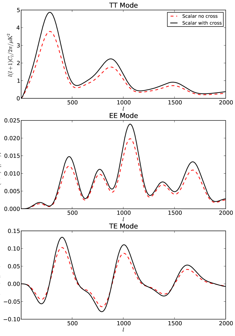
In Figure 1 we show the effect that the cross-correlation between and has on the CMB. Despite it being an anti-correlation we can see that it boosts power on all scales, as many of the perturbations are effectively sourced by the Lorentz force .
VII.3 Numerical Calculation
In Figure 2 we plot the four CMB power spectra for primordial magnetic fields. We use the constraint of Yamazaki et al. (2006), of at a scale of , with a realistic neutrino mass taken from the recent constraints of Reid et al. (2009). We include both the compensated modes for all three perturbation types as well as the passive modes. Note that within this paper we assume that the magnetic perturbations are uncorrelated with the primary sources of anisotropy in the CMB.
There is currently no leading theory of the formation of primordial magnetic fields, though there is much work suggesting their production could be around the electroweak phase transition Baym et al. (1996) at , or from just after the Quark-Hadron phase transition de Souza and Opher (2008); da Silva de Souza and Opher (2009) at . However, to produce a scale-invariant spectrum we are likely to need some kind of acausal inflationary method Bertolami and Mota (1999), though many often struggle to produce large enough magnetic fields. For an unknown inflationary mechanism the exact time and details of magnetic field production are unclear, however, for illustration we believe that the electroweak transition provides a useful bound on the latest production time, and reheating (at temperature , about the GUT scale) a bound on the earliest. This gives –. Any magnetic perturbations directly generated during inflation will source passive modes which are essentially just a component of the primordial spectra.
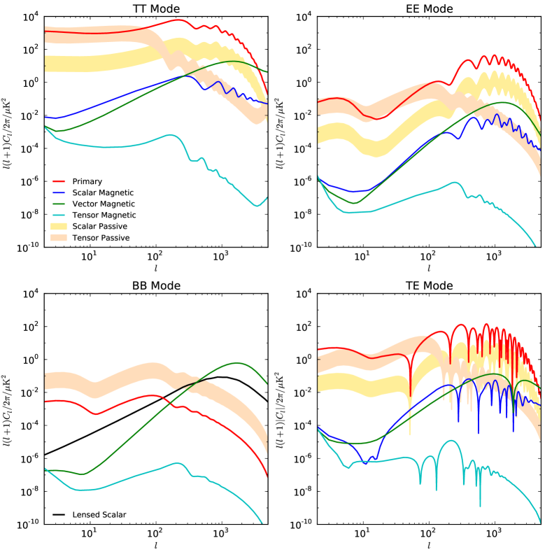
Our CMB power spectrum results are in broad agreement with previous work Paoletti et al. (2008); Lewis (2004) in the cases where the results have been calculated.
The most significant magnetic contributions to the CMB come from the tensor passive modes in all four power spectra. This is at the level of 10 percent for the temperature anisotropies and around an order of magnitude greater than the primordial gravitational wave contribution to the B-mode polarisation. The compensated vector mode is important on very small scales in the temperature power spectrum Subramanian and Barrow (2002), though here we also have to cope with significant secondary contributions from SZ111Recent work has suggested a strong constraint from the magnetic mode contribution to the SZ effect Tashiro and Sugiyama (2009) and CMB lensing. The vector mode also leaves a clear signature in the B-mode polarization spectrum on small scales, with a comparable amplitude but different shape to the secondary signal expected from CMB lensing.
Its large amplitude at low multipoles mean that the passive mode may provide stronger constraints on any primordial magnetic field than the compensated mode, though the relative amplitude between the two is uncertain due to the unknown epoch of magnetic field production (but the dependence is only logarithmic). Using current WMAP temperature data, the passive modes should constrain the magnetic field to lower than the current linear-theory CMB-only limit of Yamazaki et al. (2006). Planck B-mode data will only enhance this. The effectiveness of these CMB constraints will be limited by: secondary effects at small scales obscuring the compensated vector mode; and confusing primordial tensor modes with the passive modes on large scales (with a large cosmic variance). We should also note that as the amplitude of the power spectra scales like , improving the upper limits on the magnetic modes, translates into much weaker improvements in the magnetic field strength constraints.
The results of Kojima et al. (2008) suggested that the presence of massive neutrinos led to a significant enhancement in power in the compensated modes at the largest scales. Whilst we see an see an increase in power on large scales due to massive neutrinos, the effect we calculate is much less significant (by about five orders of magnitude). We believe this effect is due to a numerical issue with tight-coupling which we discuss in detail in Section VIII.1.
VIII Numerical Issues
VIII.1 Tight Coupling
To derive a tight coupling approximation for tensors, we take the evolution equations for the CMB temperature and E-mode polarization quadrupole
| (105) |
and
| (106) |
To obtain an equation for , we rearrange these two equations, and substitute for to give
| (107) |
Looking at this, we see that for small and small , the temperature quadrupole is also small, though we don’t show it this is also true for the E-mode quadrupole. Physically this can be interpreted as the photons are tightly coupled to the baryons if there are many scatterings within a wavelength of the perturbation, and there are many scatterings across the horizon size. Rearranging the equation for higher temperature moments
| (108) |
we see that higher moments are suppressed by factors of , that is . If we want to only retain terms up to first order in , this allows us to ignore higher moments in (107). Noting that by the same argument, we can drop all terms leaving
| (109) |
If both and are small, then the and terms in the right hard bracket are small corrections to the value of overall and we can neglect them leaving
| (110) |
the standard tight-coupling approximation for the tensors.
The problem within CAMB (Feb 2009 version) is that for tensor modes with small it uses the tight coupling approximation no matter what the value of . This clearly invalidates the tight coupling approximation, but it does not manifest itself for standard models as most of the quantities we are interested in are proportional to anyway, and thus the overall error is small (generally much smaller than 1 percent on the largest scale ’s).
As can be seen from the initial conditions in Appendix B, the growth of modes like the tensor compensated magnetic mode is modified and they grow proportional to with an effective wavenumber and thus on very large scales . This degenerate evolution ensures that the growth of large scale perturbations remains large, and thus there is a large error from the tight coupling approximation.
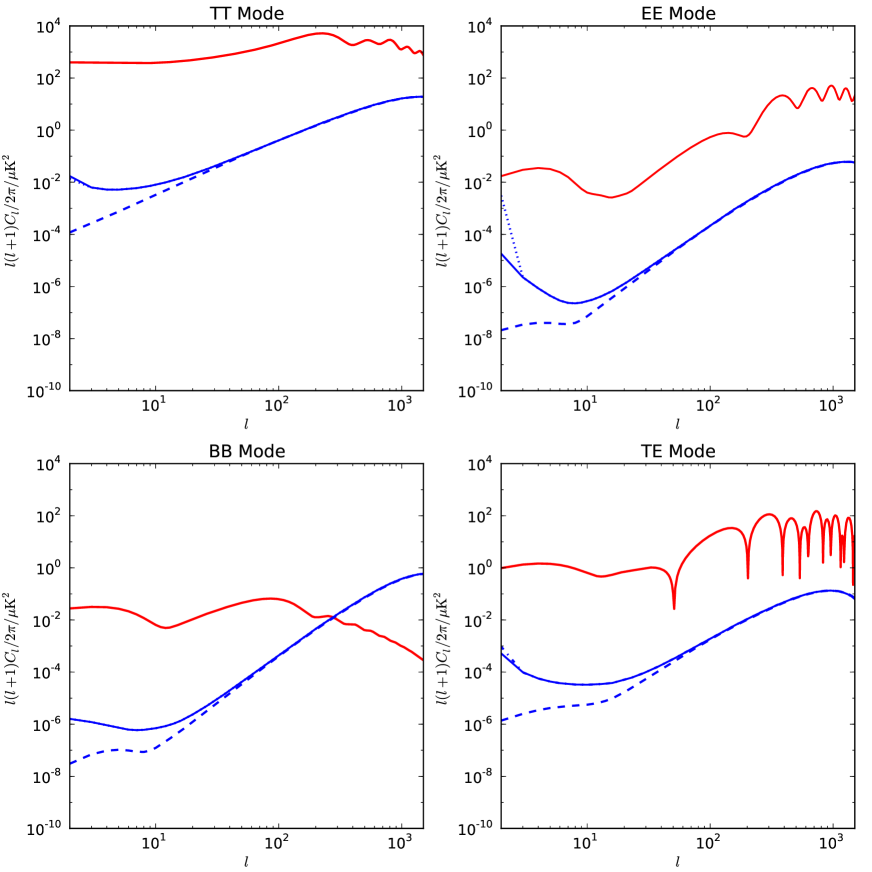
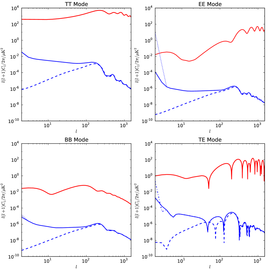
In Fig. 3 and Fig. 4 we show the vector and tensor contributions to the four CMB power spectra before and after correcting the tight coupling behaviour. As we can see this has significant effects, most notably on the tensor contribution to the EE mode power spectrum, compared to the default behaviour of CAMB. This explains the tremendous increase in large scale -mode power seen in the results of Kojima et al. (2008) where we have used the same total neutrino mass , magnetic field strength and magnetic spectral index . Our calculation shows that, even at the lowest multipoles, the tensor compensated magnetic mode is significantly lower amplitude than the primary scalar adiabatic spectrum, and remain subdominant to the compensated vector mode.
VIII.2 Early-Time Numerical Instabilities
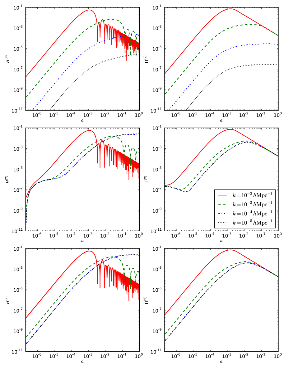
In Fig. 5 we show the evolution of the tensor perturbations of several different large scales for the compensated magnetic mode. The top set of panels show the behaviour in the presence of massless neutrinos, and we see the slowly growing scale-dependent evolution of both the gravitational waves and the total anisotropic stress. The middle panels show the output of CAMB when evolving massive neutrinos, illustrating a fundamental problem when numerically evolving these perturbations. To evolve neutrino quantities such as the anisotropic stress, we need to evolve the distribution function perturbation at a fixed set of points , then we numerically integrate over the points to calculate the desired quantity. For the standard modes this approach is fine, however, in the case of the compensated magnetic mode, the initial cancellation is at the order of , and require numerical accuracy at this level to calculate the anisotropic stress correctly. As well as simple numerical accuracy, we must integrate well into the tail of the distribution to include all contributions up to , this requires an increase in the range of values integrated from up to around .
One way to obtain the numerical accuracy would be to simply increase the number of points over which we integrate. However, combined with the required increase in range, this requires a significant increase in the number of integration points. We use an alternative approach, using our mass expansion of the Boltzmann hierarchy. At early times we directly evolve the integrated moments and use this to calculate the anisotropic stress. As the neutrinos start to become non-relativistic, our mass expansion becomes inaccurate and so before this we switch to using the full distribution function. By this time the level of cancellation is within the numerical accuracy of the integration and the total anisotropic stress is accurate. The results of this are shown in Fig. 5.
Such an approach is essential to accurately model the behaviour of massive neutrinos in the early Universe, however for calculating CMB power spectra the correctons are sub-percent level and simply increasing the range and number of integration points is sufficient.
IX Conclusion
In this paper we have developed an integrated Boltzmann hierarchy for analysing massive neutrinos in the early Universe which is accurate to second order in the mass. We have calculated the leading order mass corrections to the initial series solutions for the regular perturbation modes, and also demonstrated its use for accurately evolving massive neutrinos in the early Universe.
We have made a detailed analysis of the effects of the primordial magnetic fields on the CMB. In our examination of the statistics of the magnetic field perturbations we have included an often neglected cross-correlation term between the two scalar-perturbations. This serves to increase the power in the CMB from the compensated mode by around 25 percent at all scales. We also demonstrate that one of the standard approximations to the statistics can give an amplitude around a factor of five smaller than a more accurate result, reinforcing the need to move to more advanced results.
We accurately calculate the contributions of the various magnetic modes (both passive and compensated to the CMB). By correcting some numerical issues we come to different conclusions to Kojima et al. (2008). Whilst we agree that there is an enhancement to the large scale power spectra (especially E-mode polarization) caused by massive neutrinos, we find a much smaller amplitude; too small to enhance prospects of detecting primordial magnetic fields. Our work suggests that the passive modes are likely to dominate the compensated modes with a power spectrum amplitude several orders of magnitude greater at large scales. With the magnetic field we have used they are around 10 percent of the primary spectra, and this suggests that they will provide the biggest constraint on any primordial magnetic field in the near future, adding in a small gravitational wave like component with a blue spectral index. However unlike the compensated mode, such modes are dependent on the details of the magnetic field production, though quite weakly, and cannot provide model independent constraints on the magnetic field in the same manner as the compensated modes.
The Mathematica notebooks to calculate the magnetic mode amplitudes, and the initial conditions can be found at http://camb.info/jrs/. Our modifications to CAMB to calculate the compensated magnetic modes are at the same location.
Acknowledgements
We would like to thank Anthony Challinor for useful discussion. JRS is supported by an STFC Studentship, and AL by an STFC Advanced Fellowship.
Appendix A Higher-order mass expansion
We define a scaled mass
| (111) |
so the ratio of massive and massless neutrino densities is given by
| (112) |
where
| (113) |
Performing an expansion of in the mass by performing a series expansion of the square root inside the integral is not valid since is not much smaller than over the full range of the integral. Instead we split up the integral at a point (where ) so that
| (114) |
where
| (116) | |||
The result is independent of , and evaluates numerically to
| (118) |
Thus the next term above the leading mass correction we consider in the paper is . A similar approach can be followed for a mass expansion of the pressure using
| (119) |
Appendix B Initial Conditions
Here we present initial series solutions for the regular modes for scalar, vector and tensor perturbations in cosmology. We allow for two significantly different neutrino mass eigenstates, allowing us to describe most of the possibilities of the neutrino mass hierarchy. The solutions are correct to order in the neutrino mass. For space we have only included the terms up to second order or the first non-zero term up to order .
We include the standard matter species which we generally denote with subscripts: photons (), baryons (), cold dark matter (), massless neutrinos () and massive neutrinos (). Our solutions are for after neutrino decoupling; we discuss the pre-decoupling behaviour in the presence of magnetic fields in the Section VII.1. To solve the evolution of the background equation we solve the Friedmann equations for the scale factor. The solution to order in the neutrino mass is
| (120) |
where we choose some time to fix the values of and and . We have used the standard definition of the ratio of the density of species to the critical density. In the above we also use the definition of .
To give our series solutions we will also use the definitions of , , , and .
The solutions were calculated using Mathematica, and the notebooks and relevent packages used can be found at http://camb.info/jrs.
B.1 Scalar Initial Conditions
There are six regular scalar modes, one adiabatic, four isocurvature, and one magnetic. For comparison to other results we give our solutions in the synchronous gauge Bucher et al. (2000); Paoletti et al. (2008) with the standard potentials and , commonly used for its numerical robustness. This has the further advantage that the neutrino velocity isocurvature mode is completely regular as Bucher et al. (2000). We also give the Bardeen potentials used in the text and .
Adiabatic Mode
CDM Isocurvature Mode
Baryon Isocurvature Mode
Baryon isocurvature modes are essentially observationally indistinguishable from a rescaled CDM isocurvature mode. This is because the compensated mode (with ) gives only a small contributions at small scales, primarily from the baryon pressure and second order effects Gordon and Lewis (2003).
Neutrino Isocurvature Mode
Neutrino Velocity Isocurvature Mode
Despite the apparent singularities in the potentials and , the mode is physical with a regular comoving curvature perturbation. However, as the neutrinos are strongly coupled to the photons prior to decoupling it is challenging to find a mechanism to source this mode.
In theory we can define isocurvature modes in the neutrino anisotropic stress and higher multipole moments, though with no reasonable mechanism to produce them we will omit them.
Compensated Magnetic Modes
For the compensated magnetic mode, we treat it like an isocurvature mode with at very early times. For the density sourced modes this gives
The anisotropic stress sourced modes are
B.2 Vector Initial Conditions
There are two regular vector modes, a vorticity mode which is the vector equivalent of the neutrino velocity isocurvature mode, and a magnetic mode compensating the magnetic anisotropic stress . We give the solutions in terms of the gauge invariant variables used earlier.
Vorticity Mode
For the same reasons as the neutrino velocity mode, the existence of this type of perturbation is highly unlikely.
Compensated Magnetic Mode
B.3 Tensor Initial Conditions
Only the photons and neutrinos can support tensor perturbations to their energy momentum tensors and at times long before recombination the photon anisotropic stress is negligible. Thus the species affecting the tensor evolution are the neutrinos, and the magnetic fields. This leaves us with one standard tensor mode, the gravitational wave mode, and a compensated magnetic mode.
Gravitational Wave Mode
Compensated Magnetic Mode
References
- Kulsrud and Zweibel (2008) R. M. Kulsrud and E. G. Zweibel, Reports on Progress in Physics 71, 046901 (2008), arXiv:0707.2783.
- Wolfe et al. (2008) A. M. Wolfe, R. A. Jorgenson, T. Robishaw, C. Heiles, and J. X. Prochaska, Nature 455, 638 (2008), arXiv:0811.2408.
- Bernet et al. (2008) M. L. Bernet, F. Miniati, S. J. Lilly, P. P. Kronberg, and M. Dessauges-Zavadsky (2008), arXiv:0807.3347.
- Widrow (2002) L. M. Widrow, Reviews of Modern Physics 74, 775 (2002), arXiv:astro-ph/0207240.
- Lee et al. (2009) J. Lee, U.-L. Pen, A. R. Taylor, J. M. Stil, and C. Sunstrum (2009), arXiv:0906.1631.
- Yamazaki et al. (2006) D. G. Yamazaki, K. Ichiki, T. Kajino, and G. J. Mathews, ApJ 646, 719 (2006), arXiv:astro-ph/0602224.
- Paoletti et al. (2008) D. Paoletti, F. Finelli, and F. Paci, ArXiv e-prints (2008), arXiv:0811.0230.
- Lewis (2004) A. Lewis, Phys. Rev. D 70, 043011 (2004), arXiv:astro-ph/0406096.
- Kojima et al. (2008) K. Kojima, K. Ichiki, D. G. Yamazaki, T. Kajino, and G. J. Mathews, Phys. Rev. D 78, 045010 (2008), arXiv:0806.2018.
- Lesgourgues and Pastor (2006) J. Lesgourgues and S. Pastor, Phys. Rep. 429, 307 (2006), arXiv:astro-ph/0603494.
- Kosowsky et al. (2005) A. Kosowsky, T. Kahniashvili, G. Lavrelashvili, and B. Ratra, Phys. Rev. D 71, 043006 (2005), arXiv:astro-ph/0409767.
- Scóccola et al. (2004) C. Scóccola, D. Harari, and S. Mollerach, Phys. Rev. D 70, 063003 (2004).
- Bardeen (1980) J. M. Bardeen, Phys. Rev. D 22, 1882 (1980), ADS.
- Durrer and Straumann (1988) R. Durrer and N. Straumann, Helv. Phys. Acta 61, 1027 (1988), arXiv:astro-ph/9311041.
- Durrer (1994) R. Durrer, Fundamentals of Cosmic Physics 15, 209 (1994), arXiv:astro-ph/9311041.
- Hu and White (1997) W. Hu and M. White, Phys. Rev. D 56, 596 (1997), arXiv:astro-ph/9702170.
- Ma and Bertschinger (1995) C.-P. Ma and E. Bertschinger, ApJ 455, 7 (1995), arXiv:astro-ph/9506072.
- Lewis and Challinor (2002) A. Lewis and A. Challinor, Phys. Rev. D 66, 023531 (2002), arXiv:astro-ph/0203507.
- Lewis et al. (2000) A. Lewis, A. Challinor, and A. Lasenby, ApJ 538, 473 (2000), arXiv:astro-ph/9911177.
- Zaldarriaga and Seljak (2000) M. Zaldarriaga and U. Seljak, ApJS 129, 431 (2000), arXiv:astro-ph/9911219.
- Barrow et al. (2007) J. D. Barrow, R. Maartens, and C. G. Tsagas, Phys. Rep. 449, 131 (2007), arXiv:astro-ph/0611537.
- Kojima et al. (2009) K. Kojima, T. Kajino, and G. J. Mathews, ArXiv e-prints (2009), arXiv:0910.1976.
- Veeraraghavan and Stebbins (1990) S. Veeraraghavan and A. Stebbins, ApJ 365, 37 (1990), ADS.
- Brown and Crittenden (2005) I. Brown and R. Crittenden, Phys. Rev. D 72, 063002 (2005), arXiv:astro-ph/0506570.
- Giovannini and Kunze (2008) M. Giovannini and K. E. Kunze, Phys. Rev. D 77, 063003 (2008), arXiv:0712.3483.
- Finelli et al. (2008) F. Finelli, F. Paci, and D. Paoletti, Phys. Rev. D 78, 023510 (2008), arXiv:0803.1246.
- Mack et al. (2002) A. Mack, T. Kahniashvili, and A. Kosowsky, Phys. Rev. D 65, 123004 (2002), arXiv:astro-ph/0105504.
- Caprini et al. (2009a) C. Caprini, R. Durrer, and E. Fenu, ArXiv e-prints (2009a), arXiv:0906.4976.
- Durrer et al. (2000) R. Durrer, P. G. Ferreira, and T. Kahniashvili, Phys. Rev. D 61, 043001 (2000), arXiv:astro-ph/9911040.
- Caprini and Durrer (2002) C. Caprini and R. Durrer, Phys. Rev. D 65, 023517 (2002), arXiv:astro-ph/0106244.
- Seshadri and Subramanian (2009) T. R. Seshadri and K. Subramanian, Phys. Rev. Lett. 103, 081303 (2009), arXiv:0902.4066.
- Caprini et al. (2009b) C. Caprini, F. Finelli, D. Paoletti, and A. Riotto, Journal of Cosmology and Astro-Particle Physics 6, 21 (2009b), arXiv:0903.1420.
- Jedamzik et al. (1998) K. Jedamzik, V. Katalinić, and A. V. Olinto, Phys. Rev. D 57, 3264 (1998), arXiv:astro-ph/9606080.
- Subramanian and Barrow (1998) K. Subramanian and J. D. Barrow, Phys. Rev. D 58, 083502 (1998), arXiv:astro-ph/9712083.
- Durrer and Caprini (2003) R. Durrer and C. Caprini, Journal of Cosmology and Astro-Particle Physics 11, 10 (2003), arXiv:astro-ph/0305059.
- Reid et al. (2009) B. A. Reid, L. Verde, R. Jimenez, and O. Mena, ArXiv e-prints (2009), arXiv:0910.0008.
- Baym et al. (1996) G. Baym, D. Bödeker, and L. McLerran, Phys. Rev. D 53, 662 (1996).
- de Souza and Opher (2008) R. S. de Souza and R. Opher, Phys. Rev. D 77, 043529 (2008), arXiv:astro-ph/0607181.
- da Silva de Souza and Opher (2009) R. da Silva de Souza and R. Opher, ArXiv e-prints (2009), arXiv:0910.5248.
- Bertolami and Mota (1999) O. Bertolami and D. F. Mota, Phys. Lett. B455, 96 (1999), arXiv:gr-qc/9811087.
- Subramanian and Barrow (2002) K. Subramanian and J. D. Barrow, MNRAS 335, L57 (2002), arXiv:astro-ph/0205312.
- Tashiro and Sugiyama (2009) H. Tashiro and N. Sugiyama, ArXiv e-prints (2009), arXiv:0908.0113.
- Bucher et al. (2000) M. Bucher, K. Moodley, and N. Turok, Phys. Rev. D 62, 083508 (2000), arXiv:astro-ph/9904231.
- Gordon and Lewis (2003) C. Gordon and A. Lewis, Phys. Rev. D 67, 123513 (2003), arXiv:astro-ph/0212248.