Chromospheric Variability in SDSS M Dwarfs. II. Short-Timescale H$\alpha$ Variability

Abstract

We present the first comprehensive study of short-timescale chromospheric H$\alpha$ variability in M dwarfs using the individual 15 min spectroscopic exposures for $52,392$ objects from the Sloan Digital Sky Survey. Our sample contains about $10^{3}-10^{4}$ objects per spectral type bin in the range M0–M9, with a total of about $206,000$ spectra and a typical number of 3 exposures per object (ranging up to a maximum of $30$ exposures). Using this extensive data set we find that about $16\%$ of the sources exhibit H$\alpha$ emission in at least one exposure, and of those about $45\%$ exhibit H$\alpha$ emission in all of the available exposures. As in previous studies of H$\alpha$ activity ($L_{\rm H\alpha}/L_{\rm bol}$) we find a rapid increase in the fraction of active objects from M0–M6. However, we find a subsequent decline in later spectral types that we attribute to our use of a spectral type dependent equivalent width threshold. Similarly, we find saturated activity at a level of $L_{\rm H\alpha}/L_{\rm bol}\approx 10^{-3.6}$ for spectral types M0–M5, followed by a decline to about $10^{-4.3}$ in the range M7–M9. Within the sample of objects with H$\alpha$ emission, only 26% are consistent with non-variable emission, independent of spectral type. The H$\alpha$ variability, quantified in terms of the ratio of maximum to minimum H$\alpha$ equivalent width ($R_{\rm EW}$), and the ratio of the standard deviation to the mean ($\sigma_{\rm EW}/\langle{\rm EW}\rangle$), exhibits a rapid rise from M0 to M5, followed by a plateau and a possible decline in M9 objects. In particular, $R_{\rm EW}$ increases from a median value of about 1.8 for M0–M3 to about 2.5 for M7–M9, and variability with $R_{\rm EW}\gtrsim 10$ is only observed in objects later than M5. For the combined sample we find that the $R_{\rm EW}$ values follow an exponential distribution with $N(R_{\rm EW})\propto{\rm exp}[-(R_{\rm EW}-1)/2]$; for M5–M9 objects the characteristic scale is $R_{\rm EW}-1\approx 2.7$, indicative of stronger variability. In addition, we find that objects with persistent H$\alpha$ emission exhibit smaller values of $R_{\rm EW}$ than those with intermittent H$\alpha$ emission. Based on these results we conclude that H$\alpha$ variability in M dwarfs on timescales of 15 min to 1 hr increases with later spectral type, and that the variability is larger for intermittent sources. Future studies using this large sample will address the variability timescales, the variability of other chromospheric emission lines (e.g., H$\beta$, Ca II H&K), and the origin of the highest amplitude events.

1. Introduction

The study of magnetic activity in fully convective low mass stars and brown dwarfs (spectral types late-M, L, and T) has progressed in recent years from the question of whether these objects produce stable fields to a quantitative investigation of how the fields are produced and dissipated. Unlike the solar-type $\alpha\Omega$ dynamo, which operates in the transition region between the radiative and convective zones (the tachocline; Parker 1955), objects later than spectral type M3 can only support a convective dynamo. Numerical simulations of such a mechanism are still at an early stage, but they suggest that large-scale axisymmetric fields can indeed be generated in fully convective objects, at least for conditions that roughly correspond to mid-M dwarfs ($M\sim 0.3$ M_⊙; Browning 2008). Thus, observational constraints on the scale, geometry, and dissipation of the fields are essential.

Several observational techniques are now being used to address these questions, including Zeeman measurements in Stokes $I$ and $V$, which probe the strength of the integrated surface fields and their large-scale topology, respectively (Reiners & Basri 2007; Donati et al. 2008; Morin et al. 2008), and activity indicators such as radio, X-ray, and H$\alpha$ emission, which trace the dissipation of the field and hence its strength and geometry (e.g., West et al. 2004; Berger 2006; Berger et al. 2009). The activity indicators also provide insight into magnetic heating, and their temporal variability can potentially trace the field properties on small scales that are inaccessible to the Zeeman measurements. The current results from Zeeman measurements point to a transition from mainly toroidal and non-axisymmetric fields in M0–M3 dwarfs to predominantly poloidal axisymmetric fields in mid-M dwarfs (Donati et al. 2008; Morin et al. 2008), with field strength of $\sim 0.1-3$ kG (Reiners & Basri 2007; Donati et al. 2008; Morin et al. 2008). Studies of activity indicators point to a rapid decline in X-ray and H$\alpha$ activity (i.e., $L_{X,{\rm H\alpha}}/L_{\rm bol}$) at about spectral type M7, and uniform radio luminosity (i.e., increasing $L_{\rm rad}/L_{\rm bol}$) at least to spectral type L3 (Berger et al. 2009 and references therein). The disparate trends may be due to a decoupling of the magnetic fields from the increasingly neutral atmospheres, or to a shift in the magnetic field configuration.

While X-ray and radio observations provide powerful insight into the nature of the magnetic fields, H$\alpha$ chromospheric emission, which traces gas at temperatures of $\sim 10^{4}$ K, is more easily accessible for large samples as a by-product of standard optical spectroscopic observations. In recent years, large spectroscopic samples of M dwarfs have become available through dedicated studies and large-scale surveys such as the Sloan Digital Sky Survey (SDSS). These extensive samples have led to several important results concerning chromospheric activity. First, the fraction of objects that exhibit H$\alpha$ emission increases rapidly from $\sim 5\%$ in the K5–M3 dwarfs to a peak of $\sim 80-100\%$ around spectral type M7, followed by a subsequent decline to a few percent in the L dwarfs (Gizis et al. 2000; West et al. 2004, 2008). Second, while the level of activity increases with both rotation and youth in F–K stars, it reaches a saturated value of $L_{\rm H\alpha}/L_{\rm bol}\approx 10^{-3.6}$ in M0–M6 dwarfs, followed by a rapid decline to $L_{\rm H\alpha}/L_{\rm bol}\approx 10^{-5}$ by spectral type L0 (Hawley et al. 1996; Gizis et al. 2000; West et al. 2004), and a breakdown of the rotation-activity relation (Martín & Bouy 2002). Finally, a small fraction ($\lesssim 5\%$) of late-M and L dwarfs have been serendipitously observed to exhibit H$\alpha$ flares that reach the saturated emission levels found in the early-M dwarfs (Liebert et al. 2003).

To uniformly address the latter point — H$\alpha$ variability — we recently carried out spectroscopic monitoring observations of about 40 M4–M8 dwarfs with known H$\alpha$ emission (Lee et al. 2009). With observations of about 1 hr per source and a time resolution of $5-10$ min, we found that about $80\%$ of these objects exhibit H$\alpha$ variability on a wide range of timescales, ranging in amplitude from tens of percent up to a factor of about 5. Indeed, the timescale distribution for variability “events” is nearly flat from 10 min to 1 hr, with fewer events on timescales below 10 min. The variability amplitudes follow an exponential distribution with a characteristic scale of ${\rm Max(EW)/Min(EW)}-1\approx 0.7$. Finally, we found tentative evidence for increased variability with later spectral type.

Here, we extend our study of H$\alpha$ variability by three orders of magnitude using SDSS time-resolved spectroscopic data for a sample of 52,392 M0–M9 dwarfs (Knapp et al. 2009 in preparation; hereafter Paper I). For the first time we take advantage of the individual 15 min exposures, with a typical number of 3 exposures per source. Using these data we can thus probe H$\alpha$ variability on timescale of $15$ min to $\sim 1$ hr. In this paper we focus on the H$\alpha$ variability amplitudes and their relation to the H$\alpha$ activity level ($L_{\rm H\alpha}/L_{\rm bol}$) and spectral type. We also re-investigate the relation between H$\alpha$ activity and spectral type using the individual 15 min spectra, rather than the SDSS pipeline-combined spectra, which were used in previous work (West et al. 2004, 2008). In §2 we define our sample selection and describe the analysis method for measuring H$\alpha$ equivalent widths. The results for H$\alpha$ variability and activity are described in §3. Future papers will focus on the variability timescales, the highest amplitude events, the variability of other chromospheric emission lines (e.g., higher-order Balmer lines, Ca II H&K, He I lines), and the relation between chromospheric variability and various source properties, such as age.

2. Sample Selection and Data Analysis

The details of the sample selection are described in Paper I, where preliminary characteristics of the sample are also described. Here we provide a summary of our selection technique. We examined the combined spectra of all point sources in the SDSS DR7 database with $z\lesssim 19.5$, $i-z>0.2$, and $r-i>0.5$ mag (uncorrected for interstellar extinction). Using a set of spectral templates, including the cool star templates from Bochanski et al. (2007), we determined the best-fit spectral type for each object and removed all objects with stellar spectra earlier than K, or with the spectra of galaxies or quasars. We further removed spectra determined to be deficient according to the following criteria: inadequate signal-to-noise ratio; poor sky subtraction; large wavelength regions with missing data; and contamination by light from a nearby object or by emission from diffuse interstellar ionized gas. The resulting list contains 59,427 stars. After removal of stars of spectral type K, L and T, and removal of stars with subdwarf spectra, we find a total of 52,392 M dwarf stars.

Using the coordinates of these objects, and their plate and fiber identifications, we obtained the individual 15-min processed spectroscopic exposures. The total number of exposures is 205,823 with a range of $3-30$ exposures per source. The distribution of the number of exposures is shown in Figure 1.

2.1. Equivalent Width Measurements

To measure the H$\alpha$ equivalent width (EW) in each individual spectrum we follow a three-step process. First, we determine whether H$\alpha$ emission is significantly detected. We define the minimum required H$\alpha$ emission line significance as $3\sigma$ relative to the continuum level root-mean-square (rms) noise. This condition ensures that the H$\alpha$ emission line is significantly detected regardless of the signal-to-noise ratio, and hence the apparent brightness of the source (a combination of its spectral type and distance). In Figure 2 we plot the median $3\sigma$ threshold as a function of spectral type. For spectral types M0–M4 the threshold is about 1 Å, but it then climbs rapidly to about 3 Å for M6 and about 6 Å for M9. This spectral type dependent threshold inevitably leads to different H$\alpha$ detection statistics as a function of spectral type compared to previous analyses, which used a fixed threshold of 1 Å equivalent width from M0 to L0 (West et al. 2004, 2008); see §3. We note that since the continuum flux in the H$\alpha$ region declines with later spectral type, the use of a fixed equivalent width threshold allows weaker, and less significant “lines” to be counted as genuine detections. Our spectral type dependent threshold therefore provides more robust statistics on the H$\alpha$ properties at a fixed statistical significance. A total of 21,200 spectra exhibit H$\alpha$ emission at $>3\sigma$ significance ($10.3\%$ of all the available exposures).

Second, we identify exposures with possible cosmic ray hits in the H$\alpha$ line region using the standard SDSS pipeline flags. We find $1335$ exposures with such flags, or about $0.65\%$ of all spectra. From visual inspection, however, we find that in about half of the cases apparently genuine bright H$\alpha$ emission lines are flagged as cosmic rays. As a result, we perform a more robust cosmic ray rejection using one of the two following criteria in addition to the pipeline flag: (i) the flux of a flagged pixel within $\pm 2.5$ Å of the H$\alpha$ line center is more than twice the maximum unflagged pixel flux, or (ii) more than half of the pixels in the H$\alpha$ line and continuum region ($6545-6595$ Å) are flagged by the pipeline. The former criterion allows us to distinguish cosmic rays with a narrow width from genuine H$\alpha$ emission lines whose width is set by the spectral resolution. The latter criterion eliminates exposures with questionable flux measurements in the H$\alpha$ line region. Using these additional criteria we reduce the number of rejected exposures to $746$ ($0.36\%$ of all exposures).

To evaluate the statistical efficacy of this procedure in removing cosmic rays and in avoiding the removal of genuine H$\alpha$ emission lines, we estimate the cosmic ray hit fraction in $5$ Å windows located in regions of the spectra that are devoid of emission features. Using a random set of about $13,000$ objects that cover the full spectral type range of our study, we find that the expected cosmic ray hit fraction in the H$\alpha$ line region is about $0.30\%$, in good agreement with the fraction determined by our cosmic ray rejection criteria. This indicates that our sample is not biased by cosmic rays, and furthermore that we are not missing a substantial fraction of the large amplitude variability events due to cosmic ray rejection.

Finally, to measure the H$\alpha$ line equivalent width (EW) we simultaneously fit the H$\alpha$ line with a Gaussian profile and the continuum region with a third-order Legendre polynomial. The uncertainty in the equivalent width ($\sigma_{\rm EW}$) is determined over the same spectral region using the error spectrum associated with each exposure. For spectra that do not pass the $3\sigma$ threshold, we use this value as an upper limit. These upper limits are crucial for assessing the range of activity for M dwarfs that exhibit a mix of active and inactive spectra.

Example spectra with no H$\alpha$ emission, constant H$\alpha$ emission, and variable H$\alpha$ emission are shown in Figure 3.

3. Results for H$\alpha$ Activity and Variability

3.1. Detection Statistics

In our sample of 52,392 M dwarfs we find 8,223 objects ($15.7\%$) with at least one spectroscopic exposure that exhibits H$\alpha$ emission. This is verified by the independent analysis presented in Paper I, which used the combined spectra. The detection fraction as a function of spectral type is shown in Figure 4. For comparison, we also show the detection fractions from West et al. (2004) who used the pipeline-combined SDSS spectra and a fixed 1 Å detection threshold. As in previous studies, we find a rapid rise in the H$\alpha$ detection fraction from a level of a few percent in the range M0–M3 to about $20\%$ in M4. However, beyond spectral type M4 our results diverge from previous studies. Namely, we find that the detection fraction rises to a peak of about $40\%$ in M5–M6, and subsequently declines steadily to about $10\%$ in M9. This is in contrast to the continued rise from M4 to M8 (with a peak fraction of nearly $100\%$) found by West et al. (2008). This divergence is largely due to our spectral type dependent detection threshold (Figure 2). We demonstrate that this is the case by applying our threshold to the distributions of $L_{\rm H\alpha}/L_{\rm bol}$ from West et al. (2004), using their equivalent width conversion factors. We find that the resulting reduction in active fraction is about $15-30\%$, and it explains the difference for spectral types M5–M7. We still find a difference of about $20\%$ in the M8 and M9 bins. It is possible that the continued rise found by West et al. (2004) and West et al. (2008) was due to further contamination caused by their use of a fixed equivalent width threshold.

Of the 8,223 objects with at least one active spectrum, $45\%$ exhibit H$\alpha$ emission in all of the available exposures. The fraction of active objects as a function of the H$\alpha$ detection fraction is shown in Figure 5. This distribution does not take into account the fraction of objects in the sample with various numbers of exposures (Figure 1). For example, the peaks at H$\alpha$ detection fractions of $1/3$, $2/3$, and $3/3$ reflect the large number of objects with 3 exposures. Conversely, the low fraction of objects with H$\alpha$ detection fractions of $80-95\%$ simply reflects the small number of objects with a sufficiently large number of exposures to populate these bins (i.e., more than 5 exposures).

Even without correcting for this effect we find that for the objects with a small number of exposures ($3-5$), which occupy well defined bins, there is a systematic decline in the fraction of objects as a function of increased H$\alpha$ detection fraction. For example, the bins corresponding to $1/3$ and $2/3$ H$\alpha$ detection fractions (dominated by objects with 3 exposures) exhibit a decline in the fraction of active objects from $3.0\%$ to $1.7\%$. Similarly, there is a systematic decline in the fraction of stars with H$\alpha$ detections fractions of $1/4$, $2/4$, and $3/4$ (with values of $1.1\%$, $0.5\%$, and $0.5\%$, respectively), and a decline for objects with detection fractions of $1/5$ to $4/5$ from $0.7\%$ to $0.2\%$. We note that the rise at $100\%$ detection fraction partly reflects the combined contribution from sources with a wide range of exposure numbers, but also appears to be a genuine effect (some of the objects in this bin have steady H$\alpha$ emission; see Figure 3). The decrease in the fraction of objects as a function of increased H$\alpha$ detection fraction may reflect a typical timescale for the variability, such that variability on a $\sim 15$ min timescale is more common than on $\sim 0.5-1$ hr timescale.

To appropriately normalize the distribution for the fraction of objects with different numbers of exposures, we divide each H$\alpha$ detection fraction bin by the number of sources that can potentially populate this bin. For example, the bin at an H$\alpha$ detection fraction of 0.5 is normalized by the total number of sources with an even number of exposures, while the bin centered at 0.35 is normalized by the number of objects with exposure numbers divisible by 3. The resulting normalized distribution is shown in Figure 6. We find a relatively uniform distribution below an H$\alpha$ detection fraction of about 1/3 at a level of about $4\%$, followed by a decline to about $1-2\%$ for detection fractions of $0.4-0.95$; the number of objects with an H$\alpha$ detection fraction of 1 remains unchanged by definition.

These detection statistics alone already point to a significant level of variability in M dwarfs. Even if we make the most conservative assumption that all of the objects with a $100\%$ H$\alpha$ detection fraction are non-variable, the fraction of all M dwarfs with variable H$\alpha$ emission is at least $8.6\%$.

3.2. Activity

Before we turn to a discussion of the H$\alpha$ variability, we investigate the H$\alpha$ activity trends. A comprehensive analysis of M dwarf H$\alpha$ activity as a function of spectral type based on SDSS pipeline-combined spectra was presented by West et al. (2004) and West et al. (2008). In Figure 7 we plot $L_{\rm H\alpha}/L_{\rm bol}$ as a function of spectral type for each object. We use both the median and the maximum values, and find similar trends. The median $L_{\rm H\alpha}/L_{\rm bol}$ value for spectral types M0–M4 is roughly constant at $10^{-3.6}$, followed by a decline to a value of about $10^{-4.3}$ in M7–M9. These values are similar to those found by West et al. (2004). For the distribution of maximum $L_{\rm H\alpha}/L_{\rm bol}$ we find a nearly constant value $10^{-3.5}$ for M0–M4, followed by a decline to $10^{-4.1}$ in M7–M9. Thus, the maximum $L_{\rm H\alpha}/L_{\rm bol}$ values follow the same trend as the median values, but the difference between the median and maximum values appears to increase with later spectral type, indicative of an increase in the H$\alpha$ variability.

In Figure 8 we plot the distribution of the median $L_{\rm H\alpha}/L_{\rm bol}$ values in separate spectral type bins. The shift in the peak of the distribution to lower values as a function of later spectral type is apparent, and follows the same trend found by West et al. (2004). However, unlike these authors we find a wider dispersion in the early spectral types, primarily as a result of the significantly larger number of objects in our sample. The standard deviation values range from about 0.2 to 0.28 with no clear trend.

3.3. Variability

We now turn to the primary focus of our study — H$\alpha$ variability. We quantify the variability of each object using the ratio of maximum to minimum H$\alpha$ equivalent width, $R_{\rm EW}\equiv{\rm max(EW)/min(EW)}$, as well as the ratio of the standard deviation to the mean equivalent width, $\tilde{\sigma}_{\rm EW}\equiv\sigma_{\rm EW}/\langle{\rm EW}\rangle$. In the case of $R_{\rm EW}$ we calculate a lower limit on the variability when at least one equivalent width upper limit is available, while for $\tilde{\sigma}_{\rm EW}$ we treat the upper limits as $3\sigma$ detections; the resulting values are thus lower limits on the variability. Within the sample of objects with H$\alpha$ emission in at least one spectrum (8,223 objects) we find that about $26\%$ are consistent with steady H$\alpha$ emission within the uncertainties on the individual H$\alpha$ equivalent width measurements. This fraction is relatively uniform across the full spectral type range of M0–M9, with a possible mild decline in the later spectral types.

The distribution of $R_{\rm EW}$ values as a function of spectral type is shown in Figure 9. For each spectral type bin we separate objects with a $100\%$ detection fraction from those with at least one upper limit. In both cases we find a clear rise in $R_{\rm EW}$ as a function of spectral type, from a maximum value of about 5 for M0–M3 to about $10-17$ for M5–M8, followed by a possible decline in spectral type M9. Indeed, the objects that exhibit an H$\alpha$ variability of $\gtrsim 10$ are nearly all M5–M9 dwarfs. For the objects with a $100\%$ detection fraction we find that $1.2\%$ have $R_{\rm EW}>5$, while $0.1\%$ have $R_{\rm EW}>10$. For the objects with partial detections the fractions are $13.2\%$ and $0.5\%$, respectively. These fractions, and the overall wider distribution of $R_{\rm EW}$ values for objects with partial detections, indicate that objects with intermittent H$\alpha$ emission produce higher variability ratios than those with persistent H$\alpha$ emission. To investigate this point in more detail, we plot the distributions of $R_{\rm EW}$ values binned by detection fraction for all objects with 3 and 4 exposures (Figures 10 and 11). In both cases we find that the distributions for objects with partial detections are significantly broader than for objects with $3/3$ and $4/4$ detections.

We further find that the $R_{\rm EW}$ values follows an exponential distribution (Figure 9). For the objects with a $100\%$ detection fraction we find $N(R_{\rm EW})\propto{\rm exp}[-(R_{\rm EW}-1)/0.7]$ for $R_{\rm EW}\lesssim 4.5$. This result is identical to what we previously found for a sample of about 40 objects, which reached a maximum value of $R_{\rm EW}\approx 5$ (Lee et al. 2009). The Lee et al. (2009) sample was too small to provide constraints on larger variability ratios. Here we find that for higher ratios ($R_{\rm EW}\gtrsim 4.5$), the distribution appears to flatten to an exponential profile with $N(R_{\rm EW})\propto{\rm exp}[-(R_{\rm EW}-1)/2]$. The distribution of $R_{\rm EW}$ lower limits is generally flatter, and appears to follow a single exponential profile with $N(R_{\rm EW})\propto{\rm exp}[-(R_{\rm EW}-1)/2]$. Since these are lower limits, we conclude that the overall distribution of $R_{\rm EW}$ values for M dwarfs is an exponential with a characteristic scale of $R_{\rm EW}\gtrsim 2$.

The distribution of $R_{\rm EW}$ values for each spectral type is shown in Figure 12. The more pronounced tail of large $R_{\rm EW}$ values for spectral types $\gtrsim{\rm M4}$ is evident. In addition, we also find a systematic increase in the median of the distribution, from about 1.8 for M0–M4 to about 2.5 for M6–M9. In Figure 13 we show the same distributions, but combined for spectral types M0–M4 and M5–M9. In both cases the distributions are well fit by an exponential profile with a characteristic scale of $R_{\rm EW}-1\approx 2$ for M0–M4 and $\approx 2.7$ for M5–M9. This indicates that high amplitude variability is more common in late-M dwarfs.

Finally, similar variability trends are found using $\tilde{\sigma}_{\rm EW}$, with a steady increase from a maximum value of about 0.4 for M0 to about 1 for M5–M7, followed by a decline to about 0.7 for M8–M9 (Figure 14). As in the case of $R_{\rm EW}$, the distribution for partial detections is broader than for objects with $100\%$ detections, which follows an exponential with $N(\tilde{\sigma}_{\rm EW})\propto{\rm exp}(-\tilde{\sigma}_{\rm EW}/0.18)$. The distributions for each spectral sub-type are shown in Figure 15 and exhibit an increase in $\tilde{\sigma}_{\rm EW}$ from a median value of about 0.28 for M0–M3 to about 0.4 for M6–M9.

4. Discussion and Conclusions

We study the variability of the H$\alpha$ chromospheric emission line in M dwarfs using the individual 15 min spectroscopic exposures from SDSS for an unprecedentedly large sample of 52,392 stars. The typical timescale probed by these data is 15 min to 1 hr. About $16\%$ of the sources exhibit H$\alpha$ emission in at least one exposure, and of those about $45\%$ have H$\alpha$ emission in all of the available exposures. Only $26\%$ of all the objects with H$\alpha$ emission are consistent with steady emission, spread relatively uniformly from M0 to M9. The detection fraction as a function of spectral type exhibits the known trend of a sharp increase from a few percent in M0–M3 to tens of percent in later objects. However, unlike the results of previous studies based on SDSS pipeline-combined spectra and a fixed equivalent width threshold of 1 Å (West et al. 2004, 2008), we find a peak detection fraction of $\sim 40\%$, with a steady decline beyond M6. We attribute this trend to our use of a spectral type dependent detection threshold of $\sim 3-6$ Å ($3\sigma$) in M5–M9 objects.

The H$\alpha$ variability, quantified in terms of $R_{\rm EW}$, exhibits a substantial increase with later spectral type. For M dwarfs as a whole, the distribution of $R_{\rm EW}$ values appears to follow an exponential with $N(R_{\rm EW})\propto{\rm exp}[-(R_{\rm EW}-1)/2]$; the characteristic scale is about 2.7 for M5–M9. We also find that objects with partial detections exhibit a wider distribution of $R_{\rm EW}$ values than those with persistent H$\alpha$ emission. These results indicate that H$\alpha$ variability increases with later spectral type, even as H$\alpha$ activity declines, and that M dwarfs with intermittent H$\alpha$ activity are more variable than those with persistent H$\alpha$ emission.

In the context of chromospheric heating, these trends suggest that the magnetic energy input typically varies by a factor of about 2 on timescales of $\sim 15$ min to $\sim 1$ hr. Moreover, the increased variability as a function of later spectral type, with a particularly large increase beyond spectral types M3–M4, hints at an overall shift in the magnetic field, leading to less uniform field dissipation. Taken at face value, this conclusion suggests that the relative contribution from small scales, which are likely to dissipate on short timescales, increases for later M dwarfs. This possible trend is in conflict with preliminary results from Zeeman measurements of a few objects in the range M0–M5, which point to an increase in the relative contribution from large-scale fields (Donati et al. 2008; Morin et al. 2008; Reiners & Basri 2009). Alternatively, the increase in H$\alpha$ variability, particularly for sources with intermittent emission, may be due to an increase in the stochastic dissipation of the field in the presence of increasingly neutral atmospheres. In this scenario, heating of the bulk chromospheric plasma is suppressed by the decoupling of the field from the atmosphere (leading to a decline in $L_{\rm H\alpha}/L_{\rm bol}$), but small-scale stochastic heating still takes place (leading to an increase in the H$\alpha$ variability). The role of these two scenarios may become clearer as samples of late-M dwarfs with Zeeman measurements become available.

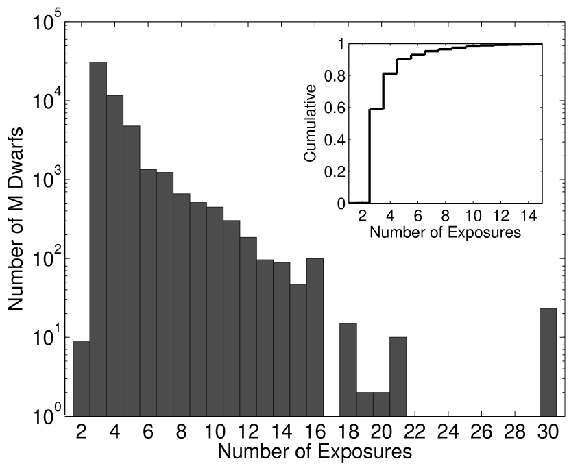
Figure 1.— Histogram of the number of M dwarfs in our sample as a function of the number of spectroscopic exposures. About $60\%$ of the objects have 3 exposures, $90\%$ have $3-5$ exposures, and $2.5\%$ have $\geq 10$ exposures.

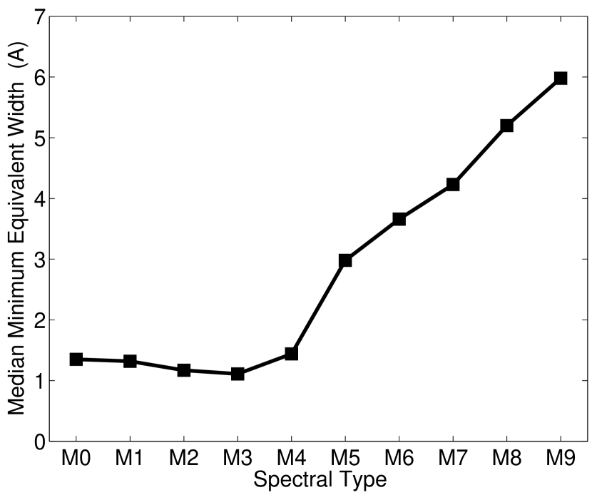
Figure 2.— Median value of the equivalent width $3\sigma$ limit as a function of spectral type. The rise in the equivalent width threshold beyond M4 reflects the decrease in signal-to-noise ratio of the spectra due to a reduction in the continuum flux level.

       

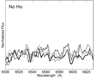
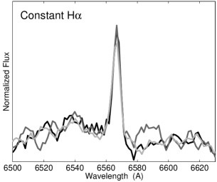
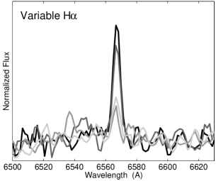
Figure 3.— Representative examples of M dwarfs with no detectable H$\alpha$ emission in any of the individual exposures (left), constant H$\alpha$ emission (center) and variable H$\alpha$ emission (right). In each panel the time sequence evolves from darker to lighter shade of gray.

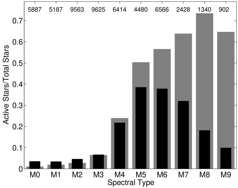
Figure 4.— Fraction of M dwarfs with at least one exposure exhibiting detectable H$\alpha$ emission as a function of spectral type. Our results are shown in black, while the results from West et al. (2004), based on SDSS pipeline-combined spectra, are shown in gray. The total number of objects in each spectral type bin from our sample is shown at the top. The divergence between the two distributions beyond spectral type M4 is primarily due to our use of a spectral type dependent equivalent width threshold (Figure 2), as opposed to a uniform threshold of 1 Å from M0-L0 in West et al. (2004); see §3.1.

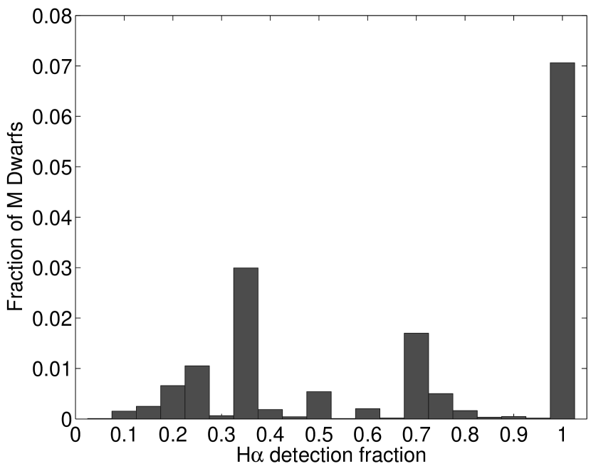
Figure 5.— Fraction of M dwarfs with detected H$\alpha$ emission binned by the fraction of exposures in which H$\alpha$ emission is detected. The peaks at 1/3, 2/3, and 1 are indicative of the large number of objects with 3 exposures (Figure 1). We do not show the large spike at zero detection fraction, corresponding to about $84\%$ of our sample.

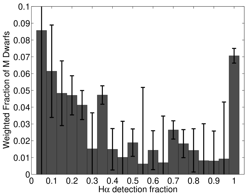
Figure 6.— Same as Figure 5 but corrected appropriately for the number of M dwarfs in the sample that can contribute to each H$\alpha$ detection fraction bin.

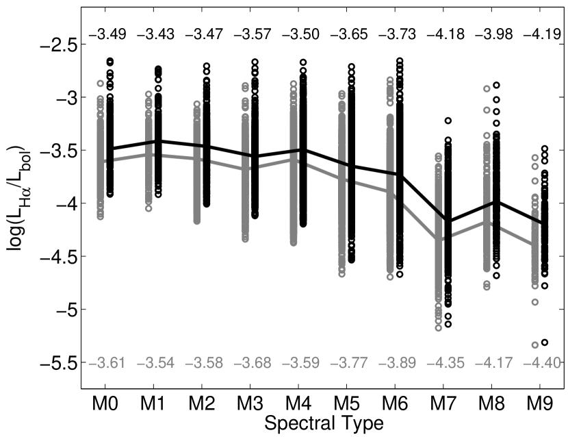
Figure 7.— H$\alpha$ activity level ($L_{\rm H\alpha}/L_{\rm bol}$) plotted as a function of spectral type. We use both the median (gray) and the maximum (black) H$\alpha$ equivalent width for each object. The lines connect the median value for each spectral type bin, and the median values are listed at the top and bottom for the maximum and median $L_{\rm H\alpha}/L_{\rm bol}$, respectively.

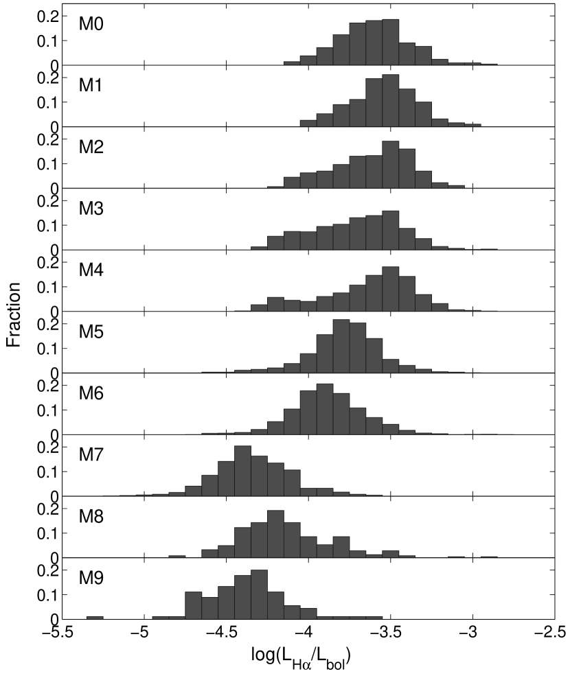
Figure 8.— Activity level ($L_{\rm H\alpha}/L_{\rm bol}$) histograms for each spectral type bin.

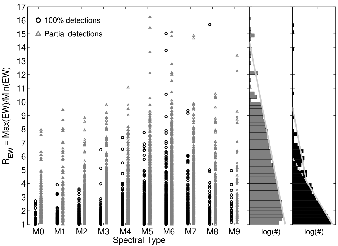
Figure 9.— Ratio of maximum to minimum equivalent width ($R_{\rm EW}$) for objects with detected H$\alpha$ emission as a function of spectral type. Circles designate objects classified as active in every exposure, while triangles mark objects with at least one active exposure and using upper limits on the minimum equivalent width for the inactive spectra. The histograms for both samples are shown in the right panels. The light gray lines are an exponential fit to these samples. The distribution for $100\%$ detection fraction appears to exhibit a break at $R_{\rm EW}\approx 4.5$.

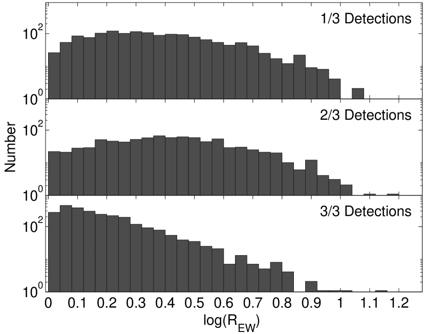
Figure 10.— Distribution of the ratio of maximum to minimum equivalent width ($R_{\rm EW}$) binned by H$\alpha$ detection fraction for all objects with 3 exposures. The $R_{\rm EW}$ values for $1/3$ and $2/3$ detections are lower limits. The objects with partial detections exhibit higher amplitude variations.

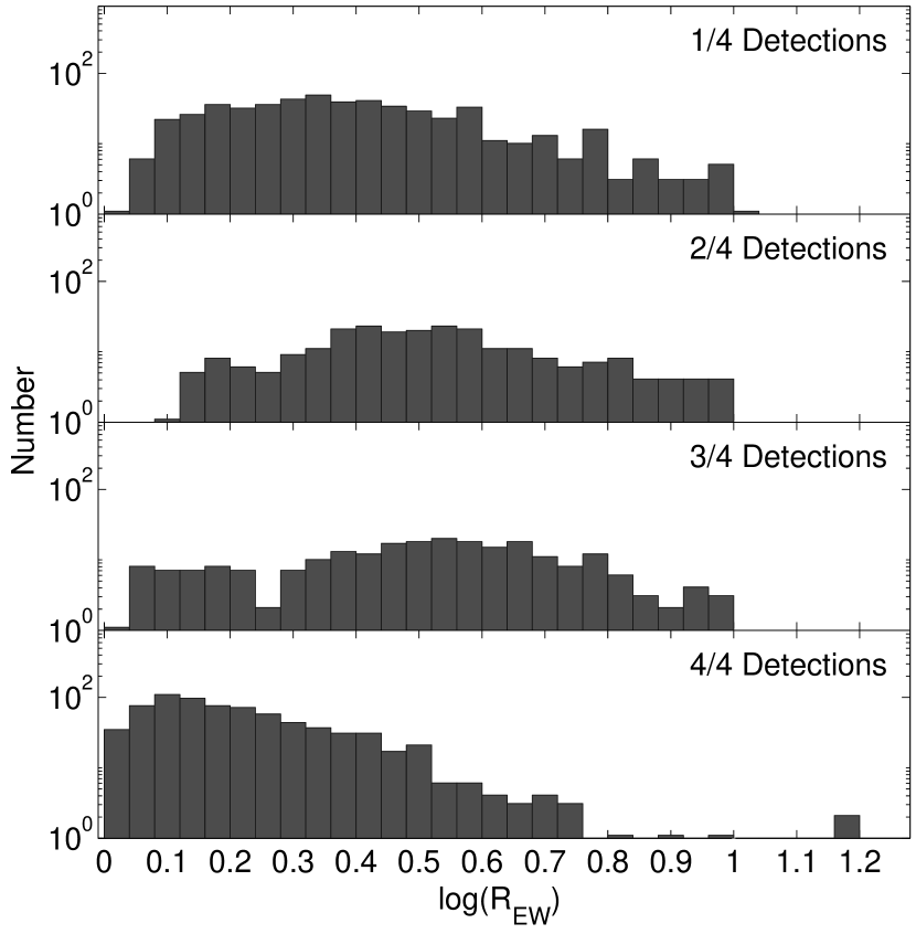
Figure 11.— Same as Figure 10 but for all objects with 4 exposures.

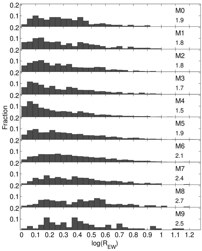
Figure 12.— Distributions of the ratio of maximum to minimum equivalent width ($R_{\rm EW}$) for each spectral type. The median $R_{\rm EW}$ value for each spectral type is listed on the right. The overall trend of increased variability with later spectral type is apparent.

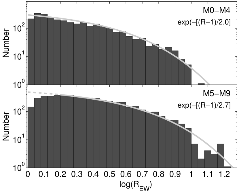
Figure 13.— Distributions of the ratio of maximum to minimum equivalent width ($R_{\rm EW}$) binned for spectral types M0–M4 (top) and M5–M9 (bottom). In both panels the gray line is an exponential fit with resulting characteristic scales of $R_{\rm EW}-1\approx 2.0$ (M0–M4) and $\approx 2.7$ (M5–M9).

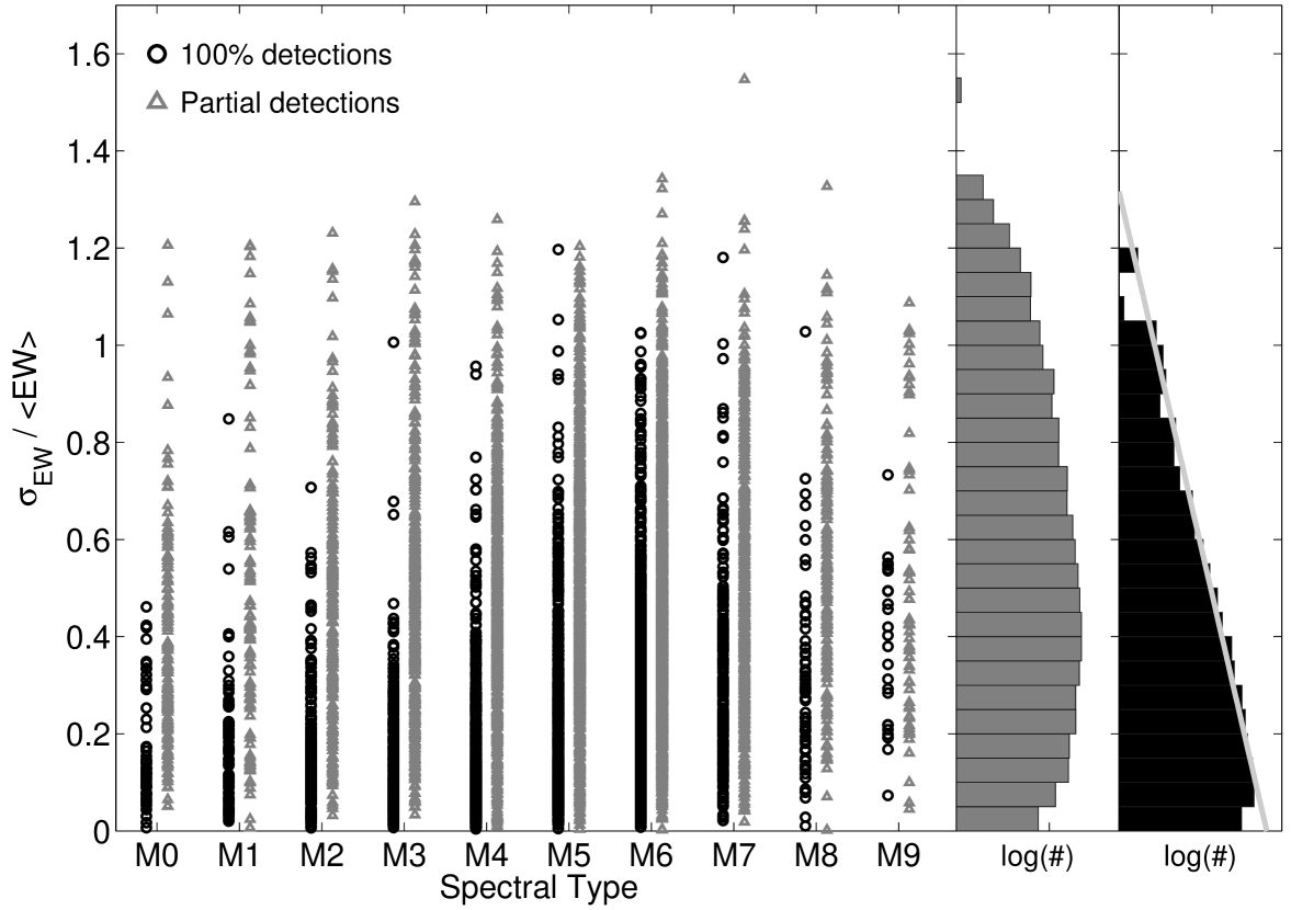
Figure 14.— Ratio of the standard deviation to the mean equivalent width for objects with detected H$\alpha$ emission as a function of spectral type. Circles designate objects classified as active in every exposure, while triangles mark objects with at least one active exposure and using upper limits on the equivalent width for the inactive spectra. The histograms for both samples are shown in the right panels. The light gray line is an exponential fit to the sample of objects with $100\%$ detection fraction.

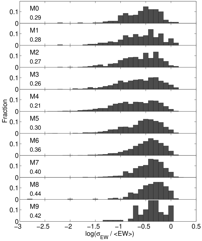
Figure 15.— Distributions of the ratio of the standard deviation to the mean equivalent width for each spectral type.

References

- Berger (2006) Berger, E. 2006, ApJ, 648, 629
- Berger et al. (2009) Berger, E., et al. 2009, ArXiv e-prints
- Bochanski et al. (2007) Bochanski, J. J., West, A. A., Hawley, S. L., & Covey, K. R. 2007, AJ, 133, 531
- Browning (2008) Browning, M. K. 2008, ApJ, 676, 1262
- Donati et al. (2008) Donati, J.-F., et al. 2008, MNRAS, 390, 545
- Gizis et al. (2000) Gizis, J. E., Monet, D. G., Reid, I. N., Kirkpatrick, J. D., Liebert, J., & Williams, R. J. 2000, AJ, 120, 1085
- Hawley et al. (1996) Hawley, S. L., Gizis, J. E., & Reid, I. N. 1996, AJ, 112, 2799
- Lee et al. (2009) Lee, K.-G., Berger, E., & Knapp, G. R. 2009, ArXiv e-prints
- Liebert et al. (2003) Liebert, J., Kirkpatrick, J. D., Cruz, K. L., Reid, I. N., Burgasser, A., Tinney, C. G., & Gizis, J. E. 2003, AJ, 125, 343
- Martín & Bouy (2002) Martín, E. L., & Bouy, H. 2002, New Astronomy, 7, 595
- Morin et al. (2008) Morin, J., et al. 2008, MNRAS, 390, 567
- Parker (1955) Parker, E. N. 1955, ApJ, 122, 293
- Reiners & Basri (2007) Reiners, A., & Basri, G. 2007, ApJ, 656, 1121
- Reiners & Basri (2009) Reiners, A., & Basri, G. 2009, A&A, 496, 787
- West et al. (2008) West, A. A., Hawley, S. L., Bochanski, J. J., Covey, K. R., Reid, I. N., Dhital, S., Hilton, E. J., & Masuda, M. 2008, AJ, 135, 785
- West et al. (2004) West, A. A., et al. 2004, AJ, 128, 426