On Asymptotic Global Error Estimation and Control of Finite Difference Solutions for Semilinear Parabolic Equations

Abstract

The aim of this paper is to extend the global error estimation and control addressed in Lang and Verwer [SIAM J. Sci. Comput. 29, 2007] for initial value problems to finite difference solutions of semilinear parabolic partial differential equations. The approach presented there is combined with an estimation of the PDE spatial truncation error by Richardson extrapolation to estimate the overall error in the computed solution. Approximations of the error transport equations for spatial and temporal global errors are derived by using asymptotic estimates that neglect higher order error terms for sufficiently small step sizes in space and time. Asymptotic control in a discrete $L_{2}$-norm is achieved through tolerance proportionality and uniform or adaptive mesh refinement. Numerical examples are used to illustrate the reliability of the estimation and control strategies.

1 Introduction

We consider semilinear parabolic partial differential equations

$$\partial_{t}u(t,x)=L(t,x)u(t,x)+g(t,x,u(t,x)),\quad t\in(0,T]\,,\;x\in\Omega\subset\mathbb{R}^{d}\,,$$ (1)

in $d\in\mathbb{N}$ space dimensions, where $L$ is an elliptic operator, and assume that an appropriate system of boundary conditions and the initial condition

$$u(0,x)=u_{0}(x)\,,\quad x\in\overline{\Omega}$$ (2)

are given. The initial boundary value problem is assumed to be well posed and to have a unique continuous solution $u(t,x)$.

The method of lines is used to solve (1) numerically. We first discretize the PDE in space by means of finite differences of order $q>1$ on a (possibly non-uniform) spatial mesh $\Omega_{h}$ and solve the resulting system of ODEs using existing time integrators. For simplicity, we shall assume that this system of time-dependent ODEs can be written in the general form

$$\begin{array}[]{rll}U^{\prime}_{h}(t)&\!=\!&F_{h}(t,U_{h}(t))\,,\qquad t\in(0,T]\,,\\[5.69046pt] U_{h}(0)&\!=\!&U_{h,0}\,,\end{array}$$ (3)

with a unique solution vector $U_{h}(t)$ being a grid function on $\Omega_{h}$. Let

$$R_{h}:\,u(t,\cdot\,)\rightarrow(R_{h}u)(t)$$ (4)

be the usual restriction operator defined by $(R_{h}u)(t)=(u(t,x_{1}),\ldots,u(t,x_{N}))^{T}$, where $x_{i}\in\Omega_{h}$ and $N$ is the number of all mesh points. Then we take as initial condition $U_{h,0}=R_{h}u(0)$.

To simplify the following derivations, we assume that $F_{h}$ is given by

$$F_{h}(t,U_{h})=L_{h}(t)U_{h}+G_{h}(t,U_{h})$$ (5)

with a finite difference approximation $L_{h}$ of $L$, and $G_{h}(t,R_{h}u)=R_{h}g(t,\cdot,u(t,\cdot))$.

To solve the initial value problem (3), we apply a numerical integration method of order $p\geq 1$ at a certain time grid

$$0=t_{0}<t_{1}<\cdots<t_{n}<\cdots<t_{M-1}<t_{M}=T\,,$$ (6)

using local control of accuracy. This yields approximations $V_{h}(t_{n})$ to $U_{h}(t_{n})$, which may be calculated for other values of $t$ by using a suitable interpolation method provided by the integrator. The global time error is then defined by

$$e_{h}(t)=V_{h}(t)-U_{h}(t)\,.$$ (7)

Numerical experiments in [5] for ODE systems have shown that classical global error estimation based on the first variational equation is remarkably reliable. In addition, having the property of tolerance proportionality, that is, there exists a linear relationship between the global time error and the local accuracy tolerance, $e_{h}(t)$ can be successfully controlled by a second run with an adjusted local tolerance. Numerous techniques to estimate global errors are described in [12]. A comparison of various adaptive grid methods for partial differential equations and implementation issues are presented in [14, 15].

In order for the method of lines to be used efficiently, it is necessary to take also into account the spatial discretization error. Defining the spatial discretization error by

$$\eta_{h}(t)=U_{h}(t)-(R_{h}u)(t)\,,$$ (8)

the vector of overall global errors $E_{h}(t)=V_{h}(t)-(R_{h}u)(t)$ may be written as sum of the global time and spatial error, that is,

$$E_{h}(t)=e_{h}(t)+\eta_{h}(t)\,.$$ (9)

We assume that $u(t,x)$ is $(q+2)$-times continuously differentiable with respect to $x$ and $(p+1)$-times continuously differentiable with respect to $t$. Then, with maximum step sizes $h_{max}$ in space and $\tau_{max}=\max_{i=0,\ldots,M-1}(t_{n+1}-t_{n})$ in time it holds for the global space and time error that $\|\eta_{h}(t_{n})\|=\mathcal{O}(h_{max}^{q})$ and $\|e_{h}(t_{n})\|=\mathcal{O}(\tau_{max}^{p})$, $n=1,\dots,M$, respectively.

Although a posteriori error estimates and adaptive algorithms for the efficient solution of parabolic problems are well established (see e.g. [3, 8] and references therein), the separation of global time and spatial discretization errors is still a challenge. First experiences to estimate and balance the spatial discretization error and the error due to time integration of the ODEs within the method of lines have been made by Schönauer, Schnepf, and Raith [10]. In their control strategy, the spatial mesh is initially chosen and remains fixed. The spatial truncation error is designated to be the level to which the local time error must be adapted. Lawson, Berzins, and Dew [7] proposed to additionally control the local time error with respect to the contribution of the existing error from the previous time steps to the global error at the end of the next time step. The error in time is enabled to vary in relation to the spatial discretization error, ensuring that the method of lines with a fixed spatial mesh is being used efficiently. A successful attempt to assess and to equilibrate the individual discretization errors with respect to a given quantity of interest has been made by Schmich and Vexler [9]. An adjoint linear parabolic problem has to be solved backwards in time to derive useful error bounds, which are used to enhance the resolution in time and space to meet a user-prescribed accuracy tolerance.

It is the purpose of this paper to present a new asymptotic error control strategy for the global errors $E_{h}(t)$, based on asymptotic estimates. We will mainly focus on reliability. So our aim is to provide error estimates $\tilde{E}_{h}(t)\approx E_{h}(t)$ which are not only asymptotically exact, but also work reliably for moderate tolerances, that is for relatively coarse discretizations. Approximations of the error transport equations for spatial and temporal global errors are derived by using asymptotic estimates that neglect higher order error terms for sufficiently small step sizes in space and time. The approximate global errors are measured in discrete $L_{2}$-norms. A priori bounds for the global error in such norms are well known, see e.g. [6, 13]. However, reliable a posteriori error estimation and efficient control of the accuracy of the solution numerically computed to an imposed tolerance level are still challenging. We achieve asymptotic global error control by iteratively improving the temporal and spatial discretizations according to asymptotic estimates of $e_{h}(t)$ and $\eta_{h}(t)$. The global time error is estimated and controlled along the way fully described in [5]. To estimate the global spatial error, we follow an approach proposed in [1] (see also [7]) and use Richardson extrapolation to set up a linearised error transport equation. Both strategies have to be combined in the right manner in order to make sure that they work reliably. Therefore, we have developed an appropriate control rule for the global spatial error. To control the overall global error more efficiently, we also consider a new fully space-time adaptive approach.

Throughout the paper we will use the terms ’approximation’ and ’estimation’ in the sense of asymptotic estimates, i.e., estimates that involve the Landau symbol $\mathcal{O}$.

The outline of this paper is as follows: In Section 2, we will linearize the transport equations for the global spatial and the global time error. These contain the residual time error and the spatial truncation error, which are approximated in Sections 3 and 4. In Section 5 we describe the discretization formulas used to approximate the solutions of the error transport equations, as well as the strategies used to adaptively adjust the time step size and the spatial mesh in dependence on the residual time error and the spatial truncation error. Now that we have approximations to the global time and global spatial error, Section 6 suggests strategies to adapt the local tolerances such that in further runs first the global time error and then the global spatial error respect some global tolerances provided by the user. Finally, numerical examples and a summary are given in Sections 7 and 8.

2 Spatial and time error

By making use of the restriction operator $R_{h}$, the spatial truncation error is defined by

$$\alpha_{h}(t)=(R_{h}u)^{\prime}(t)-F_{h}(t,(R_{h}u)(t))\,.$$ (10)

From (3) and (10), it follows that the global spatial error $\eta_{h}(t)$ representing the accumulation of the spatial discretization error is the solution of the initial value problem

$$\begin{array}[]{rll}\eta^{\prime}_{h}(t)&\!=\!&F_{h}(t,U_{h}(t))-F_{h}(t,(R_{h}u)(t))-\alpha_{h}(t)\,,\qquad t\in(0,T]\,,\\[5.69046pt] \eta_{h}(0)&\!=\!&0\,.\end{array}$$ (11)

Assuming $F_{h}$ to be twice continuously differentiable, the mean value theorem for vector functions applied to $\tilde{g}(\xi)=F_{h}(t,(R_{h}u)(t)+\xi\eta_{h}(t))$ yields

$$\begin{array}[]{rll}\eta^{\prime}_{h}(t)&\!=\!&\partial_{U_{h}}F_{h}(t,U_{h}(t))\,\eta_{h}(t)-\alpha_{h}(t)+\mathcal{O}(\eta_{h}(t)^{2}),\qquad t\in(0,T],\\[5.69046pt] \eta_{h}(0)&\!=\!&0\,.\end{array}$$ (12)

With $V_{h}(t)$ being the continuous extension of the numerical approximation to (3), the residual time error is defined by

$$r_{h}(t)=V^{\prime}_{h}(t)-F_{h}(t,V_{h}(t))\,.$$ (13)

Thus the global time error $e_{h}(t)$ fulfills the initial value problem

$$\begin{array}[]{rll}e^{\prime}_{h}(t)&\!=\!&F_{h}(t,V_{h}(t))-F_{h}(t,U_{h}(t))+r_{h}(t)\,,\qquad t\in(0,T]\,,\\[5.69046pt] e_{h}(0)&\!=\!&0\,.\end{array}$$ (14)

Again, the mean value theorem yields

$$\begin{array}[]{rll}e^{\prime}_{h}(t)&\!=\!&\partial_{U_{h}}F_{h}(t,V_{h}(t))\,e_{h}(t)+r_{h}(t)+\mathcal{O}(e_{h}(t)^{2}),\qquad t\in(0,T],\\[5.69046pt] e_{h}(0)&\!=\!&0\,.\end{array}$$ (15)

Apparently, by implementing proper choices of the defects $\alpha_{h}(t)$ and $r_{h}(t)$, solving (12) and (15) will in leading order provide approximations to the true global error. The issue of how to approximate the spatial truncation error and the residual time error will be discussed in Sections 3 and 4.

3 Approximation of the residual time error

The numerical approximation of the global time error $e_{h}(t)$ as defined in (15) requires the construction of an appropriate nearby solution $V_{h}(t)$ which is used in (13) to define the residual time error $r_{h}(t)$. The usual way is to construct an interpolatory polynomial from the numerical solutions by using Lagrange or Hermite interpolation. The latter one exploits the fact that with approximations $V_{h,n}:=V_{h}(t_{n})$ at certain time points also first derivatives $F_{h,n}:=F_{h}(t_{n},V_{h,n})$ are given. In the following we present an approach proposed in [5] to obtain the nearby solution through piecewise cubic Hermite interpolation. It turns out that this is useful as long as $1\leq p\leq 3$ with $p$ being the order of the time integration method. One step methods of order less or equal three are quite popular in the method of lines approach, since they are easy to program and the number of the arising linear systems is still of moderate size.

At every subinterval $[t_{n},t_{n+1}]$ we form

$$V_{h}(t)=V_{h,n}+A_{n}(t-t_{n})+B_{n}(t-t_{n})^{2}+C_{n}(t-t_{n})^{3},\qquad t_{n}\leq t\leq t_{n+1},$$ (16)

and choose the coefficients such that $V^{\prime}_{h}(t_{n})=F_{h,n}$ and $V^{\prime}_{h}(t_{n+1})=F_{h,n+1}$. This gives

$$V_{h}(t_{n}+\theta\tau_{n})=v_{0}(\theta)V_{h,n}+v_{1}(\theta)V_{h,n+1}+\tau_{n}w_{0}(\theta)F_{h,n}+\tau_{n}w_{1}(\theta)F_{h,n+1}$$ (17)

with $0\leq\theta\leq 1$, and

$$v_{0}(\theta)=(1-\theta)^{2}(1+2\theta),\;v_{1}(\theta)=\theta^{2}(3-2\theta),\;w_{0}(\theta)=(1-\theta)^{2}\theta,\;w_{1}(\theta)=\theta^{2}(\theta-1),$$ (18)

which imply

$$V_{h}(t_{n+1/2})=\frac{1}{2}(V_{h,n}+V_{h,n+1})+\frac{\tau_{{n}}}{8}(F_{h,n}-F_{h,n+1})$$ (19)

and

$$V^{\prime}_{h}(t_{n+1/2})=\frac{3}{2\tau_{{n}}}(V_{h,n+1}-V_{h,n})-\frac{1}{4}(F_{h,n}+F_{h,n+1}).$$ (20)

With (19) and (20) we compute from (13) the residual time error halfway the step interval as

$$\begin{array}[]{rll}\displaystyle r_{h}(t_{n+1/2})&\!=\!&\frac{3}{2\tau_{{n}}}(V_{h,n+1}-V_{h,n})-\frac{1}{4}(F_{h,n}+F_{h,n+1})\\[11.38092pt] &&-F_{h}\left(t_{n+\frac{1}{2}},\frac{1}{2}(V_{h,n}+V_{h,n+1})+\frac{\tau_{{n}}}{8}(F_{h,n}-F_{h,n+1})\right).\end{array}$$ (21)

On the other hand, assuming that $F_{h}$ is four times continuously differentiable with respect to the solution, we obtain from (13) by applying the Simpson rule that

$$\int_{t_{n}}^{t_{n+1}}r_{h}(t)~{}dt=(V_{h,n+1}-V_{h,n})-\frac{\tau_{{n}}}{6}(F_{h,n}+F_{h,n+1})\\ -\frac{2}{3}\tau_{{n}}F_{h}\left(t_{n+\frac{1}{2}},V_{h}(t_{n+1/2})\right)+\mathcal{O}(\tau_{{n}}^{5})$$ (22)

and consequently

$$\frac{1}{\tau_{{n}}}\int_{t_{n}}^{t_{n+1}}r_{h}(t)~{}dt=\frac{2}{3}r_{h}(t_{n+1/2})+\mathcal{O}(\tau_{{n}}^{4}).$$ (23)

As $r_{h}(t_{n+\frac{1}{2}})=\mathcal{O}(\tau_{n}^{\min\{p,4\}})$, the approximation (23) is useful as long as $p\leq 3$. Then, as in [5, Section 2.1] we consider instead of (15) the step size frozen version

$$\begin{array}[]{rll}{\tilde{e}}^{\prime}_{h}(t)&\!\!=\!\!&\partial_{U_{h}}F_{h}(t_{n},V_{h,n})\,{\tilde{e}}_{h}(t)+\frac{2}{3}r_{h}(t_{n+\frac{1}{2}}),\;t\in(t_{n},t_{n+1}],\;n=0,\dots,M\!-\!1,\\ {\tilde{e}}_{h}(0)&\!\!=\!\!&0\end{array}$$ (24)

to approximate the global time error $e_{h}(t)$.

Remark 3.1

When defined as above by using cubic Hermite interpolation, $r_{h}(t_{n+1/2})$ can also be used to retrieve in leading order the local error $\delta_{n+1}$ at time $t_{n+1}$ of any one-step method of order $1\leq p\leq 3$ through the relation

$$r_{h}(t_{n+1/2})=\frac{3}{2}\frac{\delta_{n+1}}{\tau_{n}}+\mathcal{O}(\tau_{n}^{p+1})\,,$$ (25)

(see also [5, Section 2.2] and [2]). So controlling $r_{h}(t_{n+1/2})$ in a local step size procedure is equivalent to the error-per-unit-step strategy (EPUS), which gives the favourite property of tolerance proportionality [11] and will also be exploited in our numerical tests. $\Diamond$

Remark 3.2

Defining the continuous extension by other means than by cubic Hermite interpolation is possible. In this case, however, the approximation (23) will in general not hold, but one could use, e.g., (22). The advantage of (23) is that $r_{h}(t_{n+\frac{1}{2}})$ can be efficiently used to control local time stepping as described in Section 5. $\Diamond$

4 Approximation of the spatial truncation error

An efficient strategy to estimate the spatial truncation error by Richardson extrapolation is proposed in [1]. We will adopt this approach to our setting.

Suppose we are given a second semi-discretization of the PDE system (1), now with doubled local mesh sizes $2h$,

$$\begin{array}[]{rll}U^{\prime}_{2h}(t)&\!=\!&F_{2h}(t,U_{2h}(t))\,,\qquad t\in(0,T]\,,\\[5.69046pt] U_{2h}(0)&\!=\!&U_{2h,0}\,.\end{array}$$ (26)

In practice, one first chooses $\Omega_{2h}$ and constructs then $\Omega_{h}$ through uniform refinement. We assume that the solution $U_{2h}(t)$ to the discretized PDE on the coarse mesh $\Omega_{2h}$ exists and is unique. For Lipschitz continuous $F_{2h}$, this condition is fulfilled. We define the restriction operator $R_{2h}^{h}$ from the fine grid $\Omega_{h}$ to the coarse grid $\Omega_{2h}$ by the identity $R_{2h}=R_{2h}^{h}R_{h}$ (where $R_{h}$ and $R_{2h}$ are defined by (4) on $\Omega_{h}$ and $\Omega_{2h}$, respectively) and set

$$\eta_{h}^{c}(t)=R_{2h}^{h}\eta_{h}(t),\quad U_{h}^{c}(t)=R_{2h}^{h}U_{h}(t),\quad V_{h}^{c}(t)=R_{2h}^{h}V_{h}(t)\,.$$ (27)

From the second assumption it follows that

$$\eta_{h}^{c}(t)=2^{-q}\eta_{2h}(t)+\mathcal{O}(h^{q+1})$$ (28)

and therefore

$$R_{2h}u(t)=\frac{2^{q}}{2^{q}-1}U_{h}^{c}(t)-\frac{1}{2^{q}-1}U_{2h}(t)+\mathcal{O}(h^{q+1})\,.$$ (29)

The relation $U_{h}^{c}(t)-U_{2h}(t)=\eta_{h}^{c}(t)-\eta_{2h}(t)$ together with (28) gives

$$U_{h}^{c}(t)-U_{2h}(t)=\frac{1-2^{q}}{2^{q}}\eta_{2h}(t)+\mathcal{O}(h^{q+1})\,.$$ (30)

The spatial truncation error on the coarse mesh $\Omega_{2h}$ is analogously to (10) defined as

$$\alpha_{2h}(t)=(R_{2h}u)^{\prime}(t)-F_{2h}(t,R_{2h}u(t))\,.$$ (31)

Substituting $R_{2h}u(t)$ from (29) into the derivative on the right-hand side and using the ODE system (26) to replace $U^{\prime}_{2h}(t)$, we obtain

$$\alpha_{2h}(t)=\frac{2^{q}}{2^{q}-1}\Big{(}({U}_{h}^{c})^{\prime}(t)-F_{2h}(t,R_{2h}u(t))\Big{)}\\ +\frac{1}{2^{q}-1}\Big{(}F_{2h}(t,R_{2h}u(t))-F_{2h}(t,U_{2h}(t))\Big{)}+\mathcal{O}(h^{q+1}).$$

As (29) and (30) imply that

$$R_{2h}u(t)=U_{h}^{c}(t)-\frac{1}{2^{q}}\eta_{2h}(t)+\mathcal{O}(h^{q+1})=U_{2h}(t)-\eta_{2h}(t)+\mathcal{O}(h^{q+1})$$

we get

$$\alpha_{2h}(t)=\frac{2^{q}}{2^{q}-1}\Big{(}(U_{h}^{c})^{\prime}(t)-F_{2h}\Big{(}t,U_{h}^{c}(t)-\frac{1}{2^{q}}\eta_{2h}(t)+\mathcal{O}(h^{q+1})\Big{)}\Big{)}\\ +\frac{1}{2^{q}-1}\Big{(}F_{2h}\Big{(}t,U_{2h}(t)-\eta_{2h}(t)+\mathcal{O}(h^{q+1})\Big{)}-F_{2h}(t,U_{2h}(t))\Big{)}+\mathcal{O}(h^{q+1}).$$ (32)

Taylor expansions yield

$$\alpha_{2h}(t)=\frac{2^{q}}{2^{q}-1}\Big{(}(U_{h}^{c})^{\prime}(t)-F_{2h}(t,U_{h}^{c}(t))\Big{)}+\mathcal{O}(h^{q+1})\,.$$ (33)

Analogously to (7), we set $e_{h}^{c}(t)\!=\!V_{h}^{c}(t)-U_{h}^{c}(t)$. Substituting $(U_{h}^{c})^{\prime}(t)$ by $R^{h}_{2h}F_{h}(t,U_{h}(t))$ and using again Taylor expansion it follows that

$$\alpha_{2h}(t)=\frac{2^{q}}{2^{q}-1}\Big{(}R^{h}_{2h}F_{h}(t,V_{h}(t))-F_{2h}(t,V_{h}^{c}(t))\Big{)}+\mathcal{O}(h^{q+1})\\ -\frac{2^{q}}{2^{q}-1}\Big{(}R^{h}_{2h}\big{(}\partial_{U_{h}}F_{h}(t,V_{h}(t))\,e_{h}(t)\big{)}-\partial_{U_{h}}F_{2h}(t,V_{h}^{c}(t))e_{h}^{c}(t)\Big{)}+\mathcal{O}(e_{h}(t)^{2})\,.$$ (34)

Assuming the term on the right-hand side involving the global time error to be sufficiently small, we can use

$$\tilde{\alpha}_{2h}(t)=\frac{2^{q}}{2^{q}-1}\Big{(}R^{h}_{2h}F_{h}(t,V_{h}(t))-F_{2h}(t,V_{h}^{c}(t))\Big{)}$$ (35)

as approximation for the spatial truncation error on the coarse mesh. To guarantee a suitable quality of the estimate (35) we shall first control the global time error with the aim that afterwards the overall error is dominated by the spatial truncation error (see Section 6).

An approximation $\tilde{\alpha}_{h}(t)$ of the spatial truncation error on the (original) fine mesh is obtained by interpolation respecting the order of accuracy (see Section 5). Thus, to approximate the global spatial error $\eta_{h}(t)$ we consider instead of (12) the step-size frozen version

$$\begin{array}[]{rll}{\tilde{\eta}}^{\prime}_{h}(t)&\!\!=\!\!&\partial_{U_{h}}F_{h}(t_{n},V_{h,n})\,{\tilde{\eta}}_{h}(t)-\tilde{\alpha}_{h}(t),\quad t\in(t_{n},t_{n+1}],\;n=0,\dots,M\!-\!1,\\[5.69046pt] {\tilde{\eta}}_{h}(0)&\!\!=\!\!&0\,.\end{array}$$ (36)

Remark 4.1

If an approximation ${\tilde{e}}_{h}(t)$ of the global time error has already been computed, we could make use of $U_{h}^{c}(t)\approx V_{h}^{c}(t){-}{\tilde{e}}_{h}^{c}(t)$ to obtain a better approximation of $\alpha_{2h}(t)$ from (33). However, we have found the following in our experiments: Using the step size frozen equations (24) and (36) together with (33) to approximate the global time and spatial error did not yield a significantly better approximation, not even in the case when the global time error was not small. Since in practice the use of formula (33) requires additional function evaluations, equation (35) appears to be more efficient. $\Diamond$

Remark 4.2

We note that special care has to be taken in the handling the spatial truncation error at the boundary when derivative boundary conditions are present. This requests interpolation adopted to the correct order of accuracy, see [1]. $\Diamond$

5 The example discretization formulas

In order to keep the illustration as simple as possible we restrict ourselves to one space dimension. For the spatial discretization of (1) we use standard second-order finite differences. Hence we have $q\!=\!2$. The discrete $L_{2}$-norm on a non-uniform mesh

$$x_{0}<x_{1}<\ldots<x_{N}<x_{N+1}\,,\quad h_{i}=x_{i}-x_{i-1}\,,\quad i=1,\ldots,N+1\,,$$ (37)

for a vector $y=(y_{1},\ldots,y_{N})^{T}\in\mathbb{R}^{N}$ is defined through

$$\|y\|^{2}=\sum_{i=1}^{N}\frac{h_{i}+h_{i+1}}{2}\,y_{i}^{2}\,.$$ (38)

Here, the components $y_{0}$ and $y_{N+1}$ which are given by the boundary values are not considered.

Adaptive time integration. The example time integration formulas are taken from [5]. For the sake of completeness we shall give a short summary of the implementation used. To generate the time grid (6) we use as an example integrator the 3rd-order, A-stable Runge-Kutta-Rosenbrock scheme ROS3P, see [3, 4] for more details. The property of tolerance proportionality [11] is asymptotically ensured through working for the local residual with

$$Est=\frac{2}{3}\,(I_{h}-\gamma\tau_{n}A_{h,n})^{-1}r_{h}(t_{n+1/2})\,,\qquad A_{h,n}=\partial_{U_{h}}F_{h}(t_{n},V_{h,n})\,,$$ (39)

where $\gamma$ is the stability coefficient of ROS3P. The common filter $(I_{h}-\gamma\tau_{n}A_{h,n})$ serves to damp spurious stiff components which would otherwise be amplified through the $F_{h}$-evaluations within $r_{h}(t_{n+1/2})$.

Let $D_{n}\!=\!\|Est\|$ and $Tol_{n}\!=\!Tol_{A}+Tol_{R}\|V_{h,n}\|$ with $Tol_{A}$ and $Tol_{R}$ given local tolerances. If $D_{n}>Tol_{n}$ the step is rejected and redone. Otherwise the step is accepted and we advance in time. In both cases, $r\tau_{n}$, where $r=(Tol_{n}/D_{n})^{1/3}$, is in leading order equal to the step size which would have led to fulfill the local tolerance condition exactly, and which we therefore want to use in the next step. To be precautious, we multiply $r\tau_{n}$ with a safety factor of $0.9$. Further, to avoid too rapid step size changes, the step size is in each step only allowed to increase by maximally 50 % and to decrease by maximally 1/3, leading overall to the new step size being determined by

$$\tau_{new}=\mbox{min}\big{(}1.5,\mbox{max}(2/3,0.9\,r)\big{)}\,\tau_{n}\,,\qquad r=(Tol_{n}/D_{n})^{1/3}\,.$$ (40)

After each step size change we adjust $\tau_{new}$ to $\tau_{n+1}=(T-t_{n})/\lfloor(1+(T-t_{n})/\tau_{new})\rfloor$ so as to avoid an unnecessarily small final time step to reach the end point $T$. The initial step size $\tau_{0}$ is prescribed and is adjusted similarly. This heuristics works quite well in practice.

The linear error transport equations (24) and (36) are simultaneously solved by means of the implicit midpoint rule, which gives approximations ${\tilde{e}}_{h,n}$ and ${\tilde{\eta}}_{h,n}$ to the global time and spatial error at time $t\!=\!t_{n}$. We use the implementations

$$\begin{array}[]{rll}(I_{h}-\frac{1}{2}\tau_{n}A_{h,n})\,\delta e_{n+1}&=&2\tilde{e}_{h,n}+\frac{2}{3}\tau_{n}r(t_{n+1/2})\,,\\ \rule{0.0pt}{11.38109pt}\tilde{e}_{h,n+1}&=&\delta e_{n+1}-\tilde{e}_{h,n}\,,\end{array}$$ (41)

and

$$\begin{array}[]{rll}(I_{h}-\frac{1}{2}\tau_{n}A_{h,n})\,\delta\eta_{n+1}&=&2\tilde{\eta}_{h,n}-\tau_{n}\tilde{\alpha}_{h}(t_{n+1/2})\,,\\ \rule{0.0pt}{11.38109pt}\tilde{\eta}_{h,n+1}&=&\delta\eta_{n+1}-\tilde{\eta}_{h,n}\,.\end{array}$$ (42)

Clearly, the matrices $A_{h,n}$ already computed within ROS3P can be reused. The spatial truncation error $\tilde{\alpha}_{2h}(t)$ at $t\!=\!t_{n+1/2}$ is given by

$$\tilde{\alpha}_{2h}(t_{n+1/2})=\frac{4}{3}\,\left(R_{2h}^{h}F_{h}\left(t_{n+1/2},V_{h}(t_{n+1/2})\right)-F_{2h}\left(t_{n+1/2},R_{2h}^{h}V_{h}(t_{n+1/2})\right)\right)\,.$$ (43)

Since $V_{h}(t_{n+1/2})$ and $F_{h}(t_{n+1/2},V_{h}(t_{n+1/2}))$ are available from the computation of $r_{h}(t_{n+1/2})$ in (21), this requires only one function evaluation on the coarse grid. The vector $\tilde{\alpha}_{2h}(t_{n+1/2})$ on the coarse mesh is prolongated to the fine mesh and is then divided by $2^{q}\!=\!4$ if the neighbouring fine grid points are equidistant, otherwise it is divided by $2^{q-1}\!=\!2$. The remaining $\tilde{\alpha}_{h}(t_{n+1/2})$ on the fine mesh are computed by interpolation respecting the order of the neighbouring spatial truncation errors.

Due to freezing the coefficients in each time step, the second-order midpoint rule is a first-order method when interpreted for solving the linearised equations (15) and (12). Thus if all is going well, we asymptotically have ${\tilde{e}}_{h,n}\!=\!e_{h}(t_{n})+\mathcal{O}(\tau_{max}^{4})$ and ${\tilde{\eta}}_{h,n}\!=\!\eta_{h}(t_{n})+\mathcal{O}(\tau_{max}h_{max}^{q})+\mathcal{O}(h_{max}^{q+1})$.

After computing the spatial truncation errors we can solve the discretized error transport equations (42) for all ${\tilde{\eta}}_{h,n}$. We shall distinguish between two different mesh adaptation approaches: (i) globally uniform and (ii) locally adaptive refinement. Although the uniform strategy may be less efficient, it is very easy to implement and therefore of special practical interest if software packages which do no allow dynamic adaptive mesh refinement are used.

Uniform spatial refinement. Let $Tol$ be a given tolerance. Then our aim is to guarantee $\|\eta_{h}(T)\|\leq Tol$. From (42), we get an approximate value ${\tilde{\eta}}_{h,M}$ for the spatial discretization error at $T$. If the desired accuracy is still not satisfied, i.e., $\|{\tilde{\eta}}_{h,M}\|>Tol$, we choose a new (uniform) spatial resolution

$$h_{new}=\sqrt[q]{\frac{Tol}{\|{\tilde{\eta}}_{h,M}\|}}\,h$$ (44)

to account for achieving $\|\eta_{h_{new}}(T)\|\approx Tol$. From $h_{new}$ we determine a new number of mesh points. The whole computation is redone with the new spatial mesh.

Adaptive spatial refinement. The main idea of our local spatial mesh control is based on the observation that the principle of tolerance proportionality can also be applied to the spatial discretization error. Multiplying all $\tilde{\alpha}_{h}(t_{n+1/2})$ in (42) by a certain constant multiplies all ${\tilde{\eta}}_{h,n+1}$ by the same constant since ${\tilde{\eta}}_{h,0}\!=\!0$. Set $Tol_{n}^{\alpha}\!=\!Tol_{A}^{\alpha}+Tol_{R}^{\alpha}\|V_{h,n}\|$ where $Tol_{A}^{\alpha}$ and $Tol_{R}^{\alpha}$ are given local tolerances and define a local estimator $A_{n}$ through

$$A_{n}^{2}=\sum_{i:\,x_{i}\in F_{h}}2h_{i}|\tilde{\alpha}_{i}(t_{n+1/2})|^{2},$$ (45)

where $F_{h}$ denotes the set of all (fine) mesh points that do not belong to the coarse mesh. Remember we have second order of the spatial truncation error in these points. If $A_{n}\leq Tol_{n}^{\alpha}$ the mesh is only coarsened. Otherwise, if $A_{n}>Tol_{n}^{\alpha}$ the mesh is improved by refinement and coarsening as well. We set $\alpha_{tol}\!=\!0.9\,Tol_{n}^{\alpha}/\sqrt{N}$ and mark all $x_{i}\in F_{h}$

$$\begin{array}[]{rll}\mbox{for refinement if }&&\sqrt{h_{i}}\,\tilde{\alpha}_{i}(t_{n+1/2})>\alpha_{tol}\\ \rule{0.0pt}{11.38109pt}\mbox{and for coarsening if }&&\sqrt{h_{i}}\,\tilde{\alpha}_{i}(t_{n+1/2})<0.1\,\alpha_{tol}\,.\end{array}$$ (46)

Grid adaptation is first performed for the coarse mesh and afterwards the fine mesh is constructed by halving each interval. If $x_{i}$ is marked for refinement the corresponding coarse grid interval is halved. Grid points are only removed if there are two equidistant neighbouring intervals the midpoints of which are marked for coarsening. Finally, the grid is smoothed such that $0.5\!\leq\!h_{i}/h_{i-1}\!\leq\!2$ everywhere. Data transfer from old to new meshes is done by cubic Hermite interpolation where the necessary first derivatives are determined from fourth order finite differences.

After mesh adaptation the local time step is redone with the new mesh. The procedure is continued until first $D_{n}\leq Tol_{n}$ and second $A_{n}\leq Tol_{n}^{\alpha}$ hold. The whole strategy aims at equidistributing the local values $\sqrt{h_{i}}\,\tilde{\alpha}_{i}(t_{n+1/2})$. Asymptotically we get

$$A_{n}\approx\left(2\sum_{i:\,x_{i}\in F_{h}}\alpha_{tol}^{2}\right)^{1/2}=\left(2\sum_{i:\,x_{i}\in F_{h}}\frac{0.81\,(Tol_{n}^{\alpha})^{2}}{N}\right)^{1/2}\approx 0.9\,Tol_{n}^{\alpha}\,,$$ (47)

where the factor $0.9$ improves the robustness of the equidistribution principle.

6 The control rules

Like for the ODE case studied in [5] our aim is to provide global error estimates and to control the accuracy of the numerically computed solution to the imposed tolerance level. Let $GTol_{A}$ and $GTol_{R}$ be the global tolerances. Then we start with the local tolerances $Tol_{A}=GTol_{A}$, $Tol_{R}=GTol_{R}$, and in the spatially adaptive case also with $Tol_{A}^{\alpha}=C_{\alpha}\,GTol_{A}$, and $Tol_{R}^{\alpha}=C_{\alpha}\,GTol_{R}$, where the factor $C_{\alpha}>1$ ensures that the residual time error is small with respect to the spatial truncation error and therefore the use of (35) is justified.

Suppose the numerical schemes have delivered an approximate solution $V_{h,M}$ and global estimates ${\tilde{e}}_{h,M}$ and ${\tilde{\eta}}_{h,M}$ for the time and spatial error at time $t_{M}\!=\!T$. We then verify whether

$$\|{\tilde{e}}_{h,M}\|\leq C_{T}C_{control}Tol_{M},\quad Tol_{M}=GTol_{A}+GTol_{R}\|V_{h,M}\|,$$ (48)

where $C_{control}\approx 1$, typically $>1$, and $C_{T}\in(0,1)$ denotes the fraction desired for the global time error with respect to the tolerance $Tol_{M}$. If (48) does not hold, the whole computation is redone over $[0,T]$ with the same initial step $\tau_{0}$ and the adjusted local tolerances

$$Tol_{A}=Tol_{A}\cdot fac,\quad Tol_{R}=Tol_{R}\cdot fac,\quad fac=C_{T}Tol_{M}/\|{\tilde{e}}_{h,M}\|.$$ (49)

Based on tolerance proportionality, reducing the local error estimates with the factor fac will reduce $e_{h}(T)$ by fac [11].

Step	Control Algorithm with Uniform Refinement in Space
Step 0	Choose global tolerances $GTol_{A}$ and $GTol_{R}$.
	Choose $C_{T}$, $C_{control}$, $h_{0}$, $q$, and $\tau_{0}$.
	Set local tolerances $Tol_{A}=GTol_{A}$ and $Tol_{R}=GTol_{R}$.
	Set $h=h_{0}$.
Step 1	Run numerical schemes to compute $V_{h,M},{\tilde{e}}_{h,M},{\tilde{\eta}}_{h,M}$.
	Compute $Tol_{M}=GTol_{A}+GTol_{R}\|V_{h,M}\|$.
Step 2	IF $\|{\tilde{e}}_{h,M}\|\leq C_{T}C_{control}Tol_{M}$ GOTO Step 3.
	ELSE set
	$fac=C_{T}Tol_{M}/\|{\tilde{e}}_{h,M}\|$, $Tol_{A}=Tol_{A}\cdot fac$, $Tol_{R}=Tol_{R}\cdot fac$
	and GOTO Step 1.
Step 3	IF $\|{\tilde{e}}_{h,M}+{\tilde{\eta}}_{h,M}\|\leq C_{control}Tol_{M}$ GOTO Step 4.
	ELSE set $h=\sqrt[q]{(1-C_{T})Tol_{M}/\|{\tilde{\eta}}_{h,M}\|}\,h$ and GOTO Step 1.
Step 4	IF $h\neq h_{0}$ compute $q_{num}$.
	ELSE set $h=2h$, run numerical schemes again and compute then
	$q_{num}$.
	IF $q_{num}\approx q$ accept fine grid solution and STOP.
	ELSE set $h_{0}=2h_{0},h=h_{0}$ and GOTO Step 1.

Table 1: Algorithmic structure of the overall control strategy when uniform refinement in space is used.

Step	Control Algorithm with Adaptive Refinement in Space
Step 0	Choose global tolerances $GTol_{A}$ and $GTol_{R}$.
	Choose $C_{T}$, $C_{control}$, $C_{\alpha}$, $q$, and $\tau_{0}$.
	Set local tolerances
	$Tol_{A}\!=\!GTol_{A}$, $Tol_{R}\!=\!GTol_{R}$, $Tol_{A}^{\alpha}\!=\!C_{\alpha}\,GTol_{A}$, and
	$Tol_{R}^{\alpha}\!=\!C_{\alpha}\,GTol_{R}$.
	Choose initial spatial mesh.
Step 1	Run numerical schemes to compute $V_{h,M},{\tilde{e}}_{h,M},{\tilde{\eta}}_{h,M}$.
	Compute $Tol_{M}=GTol_{A}+GTol_{R}\|V_{h,M}\|$.
Step 2	IF $\|{\tilde{e}}_{h,M}\|\leq C_{T}C_{control}Tol_{M}$ GOTO Step 3.
	ELSE set
	$fac=C_{T}Tol_{M}/\|{\tilde{e}}_{h,M}\|$, $Tol_{A}=Tol_{A}\cdot fac$, $Tol_{R}=Tol_{R}\cdot fac$
	and GOTO Step 1.
Step 3	IF $\|{\tilde{e}}_{h,M}+{\tilde{\eta}}_{h,M}\|\leq C_{control}Tol_{M}$ accept solution and STOP.
	ELSE set
	$fac\!=\!(1-C_{T})Tol_{M}/\|{\tilde{\eta}}_{h,M}\|$, $Tol_{A}^{\alpha}\!=\!Tol_{A}^{\alpha}\cdot fac$, $Tol_{R}^{\alpha}\!=\!Tol_{R}^{\alpha}\cdot fac$
	and GOTO Step 1.

Table 2: Algorithmic structure of the overall control strategy when adaptive refinement in space is used.

If (48) holds, we check whether

$$\|{\tilde{e}}_{h,M}+{\tilde{\eta}}_{h,M}\|\leq C_{control}Tol_{M}.$$ (50)

If it is true, the overall error $E_{h}(T)\!=\!V_{h}(T)\!-\!(R_{h}u)(t)\!=\!e_{h}(T)\!+\!\eta_{h}(T)$ is considered small enough relative to the chosen tolerance and $V_{h,M}$ is accepted. Otherwise, the whole computation is redone with the (already) adjusted tolerances (49) and an improved spatial resolution.

In the uniform case, we use the new mesh size computed from (44) with $Tol=(1-C_{T})Tol_{M}$. To check the convergence behaviour in space and therefore also the quality of the approximation of the spatial truncation error, we additionally compute the numerically observed order

$$q_{num}=\log\left(\frac{\|{\tilde{\eta}}_{h,M}\|}{\|{\tilde{\eta}}_{h_{new},M}\|}\right)\big{/}\log\left(\frac{h}{h_{new}}\right).$$ (51)

If $q_{num}$ computed for the final run is not close to the expected value $q$ used for our Richardson extrapolation, we reason that the approximation of the spatial truncation errors has failed due to a dominating global time error, which happens, e.g., if the initial spatial mesh is already too fine. Consequently, we coarsen the initial mesh by a factor two and start again. If the control approach stops without a mesh refinement, we perform an additional control run on the coarse mesh and compute $q_{num}$ from (51) with $h_{new}\!=\!2h$. It turns out that this simple strategy works quite robustly, provided that the meshes used are able to resolve the basic behaviour of the solution. The algorithmic structure of our control strategy with uniform refinement in space is given in Table 1.

In the adaptive case, we choose new local tolerances

$$Tol_{A}^{\alpha}=Tol_{A}^{\alpha}\cdot fac,\quad Tol_{R}^{\alpha}=Tol_{R}^{\alpha}\cdot fac,\quad fac=(1-C_{T})Tol_{M}/\|{\tilde{\eta}}_{h,M}\|\,,$$ (52)

and the whole computation is redone over the interval $[0,T]$. Based on tolerance proportionality, reducing the local truncation error with the factor fac will reduce $\eta_{h}(T)$ by fac. In Table 2, the algorithmic structure of our control strategy with adaptive refinement in space is displayed. Note that now the index $h$ refers to a sequence of spatial meshes adapted at each time point $t_{n}$.

Summarizing, the first check (48) and the possible second control computation serve to significantly reduce the global time error. This enables us to make use of the approximation (35) for the spatial truncation error, which otherwise could not be trusted. The second step based on suitable spatial mesh improvement attempts to bring the overall error down to the imposed tolerance. Using the sum of the approximate global time and spatial error inside the norm in (50), we take advantage of favourable effects of error cancellation. These two steps are successively repeated until the second check is successful. Additionally, if uniform mesh refinement is used we take into account the numerically observed order in space to assess the approximation of the spatial truncation error.

7 Numerical illustrations

To illustrate the performance of the global error estimators and the control strategy, we consider three test problems: (i) the highly stable heat equation with nonhomogeneous Neumann boundary conditions [1], (ii) the nonlinear convection-dominated Burgers’ equation [1, 7], and (iii) the Allen-Cahn equation modelling a diffusion-reaction problem [5]. Analytic solutions are known for all three problems. Uniform spatial refinement is studied for all three test cases. For the Burgers’ and Allen-Cahn problem, these results are compared to those obtained with adaptive refinement. We omit the corresponding results for the heat equation, since the solution is very smooth in space and hence adaptive refinement is not necessary. The challenge here is to control the fast decay in time.

We set $GTol_{A}=GTol_{R}=GTol$ for $GTol=10^{-l},l=2,\ldots,7$ and start with one and the same initial step size $\tau_{0}=10^{-5}$. Equally spaced meshes of $25$, $51$, $103$, $207$, $415$, $831$, and $1663$ points are used as initial mesh. The control parameters introduced above for the control rules are $C_{T}=1/3$, $C_{control}=1.2$, and $C_{\alpha}=10$. All runs were performed, but for convenience we only select a representative set of them for our presentation.

We define the estimated global error $\tilde{E}_{h,M}={\tilde{e}}_{h,M}+{\tilde{\eta}}_{h,M}$ at time $t=T$ and set indicators $\Theta_{est}=\|\tilde{E}_{h,M}\|/\|E_{h}(T)\|$ for the ratio of the estimated global error and the true global error, and $\Theta_{ctr}=Tol_{M}/\|E_{h}(T)\|$ for the ratio of the desired tolerance and the true global error. Thus, $\Theta_{ctr}\geq 1/C_{control}=5/6$ indicates control of the true global error.

The tables of results contain the following quantities, $Tol=Tol_{A}=Tol_{R}$ from (49), $Tol^{\alpha}=Tol_{A}^{\alpha}=Tol_{R}^{\alpha}$ from (52), $Tol_{M}=GTol\,(1+\|V_{h,M}\|)$ from (48), the estimated global error $\tilde{E}_{h,M}$, the estimated time error ${\tilde{e}}_{h,M}$, and the estimated spatial truncation error ${\tilde{\eta}}_{h,M}$. Note that we always start with $Tol=GTol$ in the first run. The ratios $\Theta_{est}$ and $\Theta_{ctr}$ serve to illustrate the quality of the global error estimation and the control. If uniform refinement in space is applied, the numerically observed order $q_{num}$ for the spatial error is given. It will be clear from the tables of results whether a tolerance-adapted run to control the global time error, a spatial mesh adaptation step or an additional control run on a coarser grid was necessary. Especially, the latter is marked by a dashed line.

$Tol$	$N$	$Tol_{M}$	$\|\tilde{E}_{h,M}\|$	$\|{\tilde{e}}_{h,M}\|$	$\|{\tilde{\eta}}_{h,M}\|$	$\Theta_{est}$	$\Theta_{ctr}$	$q_{num}$
1.00e-2	25	1.10e-2	7.14e-4	1.16e-4	8.20e-4	0.99	15.27
1.00e-2	13	1.10e-2	3.27e-3	1.24e-4	3.38e-3	0.99	3.32	2.04
1.00e-3	51	1.10e-3	1.68e-4	1.97e-5	1.86e-4	1.00	6.51
1.00e-3	25	1.10e-3	8.04e-4	2.03e-5	8.22e-4	1.00	1.36	2.02
1.00e-4	103	1.10e-4	4.27e-5	2.01e-6	4.44e-5	1.00	2.57
1.00e-4	51	1.10e-4	1.85e-4	1.96e-6	1.86e-4	1.00	0.59	2.01
1.00e-5	207	1.10e-5	1.07e-5	1.89e-7	1.08e-5	1.00	1.03
1.00e-5	103	1.10e-5	4.43e-5	1.83e-7	4.44e-5	1.00	0.25	2.01
1.00e-6	415	1.10e-6	2.67e-6	1.81e-8	2.68e-6	1.00	0.41
1.00e-6	795	1.10e-6	7.14e-7	1.83e-8	7.28e-7	1.00	1.54	2.00
1.00e-7	25	1.10e-7	8.24e-4	1.24e-9	8.24e-4	1.00	0.00
1.00e-7	2759	1.10e-7	5.91e-8	1.60e-9	6.03e-8	1.00	1.86	2.01
1.00e-7	1663	1.10e-7	1.65e-7	1.57e-9	1.66e-7	1.00	0.67
1.00e-7	2505	1.10e-7	7.20e-8	1.57e-9	7.31e-8	1.00	1.53	2.00

Table 3: Selected data for the heat equation with Neumann boundary conditions. Uniform refinement in space is used.

7.1 Heat equation with Neumann boundary conditions

This heat equation provides an example with inhomogeneous Neumann boundary conditions:

$$\partial_{t}u=\partial_{xx}u\,,\quad 0<x<1.0\,,\qquad 0<t\leq T=0.2\,,$$ (53)

and boundary conditions $\partial_{x}u=\pi\,e^{-\pi^{2}t}\cos(\pi x)$ at $x\!=\!0$ and $x\!=\!1$. The initial condition is consistent with the analytic solution $u(x,t)\!=\!e^{-\pi^{2}t}\sin(\pi x)$. Although the solution is very stable, it is not easy to provide good error estimates as stated in [1, 7].

To approximate the inhomogeneous Neumann boundary conditions we introduce artificial mesh points $x_{-1}=-h$ and $x_{N+2}=1+h$, discretize $\partial_{x}u(0)$ and $\partial_{x}u(1)$ by second order central differences, and use the approximate differential equation at the boundary to eliminate the artificial solution values. In consequence, we have global spatial order $q=2$ in all mesh points, but when interpolating the estimated spatial truncation error we have to respect that it is of first order at the boundary (see also Remark 4.2).

Due to the high stability of the problem the global time errors are much smaller than imposed local tolerances. So, control of the global time error is redundant here and control runs were only carried out in case of insufficient spatial resolutions. Table 3 shows results for various tolerances and initial meshes. We select two runs to explain the control strategy. For the third simulation, we take $GTol=10^{-4}$ and start with the local tolerance $Tol=10^{-4}$. Using $103$ mesh points in space, we run the computation and get the following approximations of the time and spatial errors: $\|{\tilde{e}}_{h,M}\|=2.01\times 10^{-6}$ and $\|{\tilde{\eta}}_{h,M}\|=4.44\times 10^{-5}$. The control checks for the time error estimate, $\|{\tilde{e}}_{h,M}\|\leq C_{T}C_{control}Tol_{M}=4.4\times 10^{-5}$, and for the global error, $\|\tilde{E}_{h,M}\|=4.27\times 10^{-5}\leq 1.32\times 10^{-4}=C_{control}Tol_{M}$, are positive, so that we already can stop after the first run. In accordance with our safety strategy, we additionally perform one run on a coarser mesh with half of the grid points, i.e., $N=51$. The numerically observed order computed from (51) is $q_{num}=2.01$. We reason that our assumption for a successful Richardson extrapolation to estimate the spatial truncation error is fulfilled and accept the numerical solution. Choosing $GTol=10^{-7}$ and $N=25$, the approximate time error is still very small, but the check for the global error, $8.24\times 10^{-4}\leq 1.32\times 10^{-7}$, obviously fails. From (44), we compute a new number of spatial mesh points, $N=2759$. Finally, the second run is successful and with the numerically observed spatial order $q_{num}=2.01$ the numerical solution is accepted.

Figure 1: Evolution of the efficiency indicators $\Theta_{est}$ (left) and $\Theta_{ctr}$ (right) for the heat equation with Neumann boundary conditions and global tolerances $GTol=10^{-i},\,i=2,\ldots,7$. Different icons represent different $GTols$. The progress in the local time tolerance $Tol$ is described by diverse colouring. Control of the true global error, i.e. $\Theta_{ctr}\geq 5/6$, is achieved in all cases. Only for higher tolerances $GTol=10^{-6},\,10^{-7}$, a second run is necessary, indicated by connected icons. The quality of the estimates is very high.

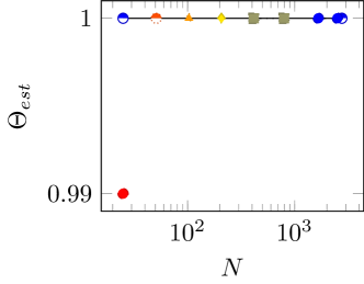
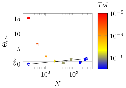
The global error estimation and control appear to work very well for this problem, where the influence of the initial mesh points is less strong. This holds also for other combinations of tolerances and initial meshes. The results are visualized in Fig. 1. Note the high quality of the estimator $\tilde{E}_{h,M}$ (and therefore also of ${\tilde{\eta}}_{h,M}$), showing that the derivative boundary condition is well resolved within the Richardson extrapolation. For the runs with tolerances $GTol\!=\!10^{-2},10^{-3},10^{-4},10^{-5}$, the order of the spatial convergence was successfully checked with a second run on the coarse mesh, that is, we can trust the first run.

$Tol$	$N$	$Tol_{M}$	$\|\tilde{E}_{h,M}\|$	$\|{\tilde{e}}_{h,M}\|$	$\|{\tilde{\eta}}_{h,M}\|$	$\Theta_{est}$	$\Theta_{ctr}$	$q_{num}$
1.00e-2	51	1.93e-2	4.30e-3	1.86e-3	2.86e-3	1.08	4.87
1.00e-2	25	1.93e-2	1.29e-2	2.21e-3	1.14e-2	0.99	1.48	2.00
1.00e-3	51	1.93e-3	2.83e-3	1.54e-4	2.74e-3	0.99	0.68
1.00e-3	75	1.93e-3	1.36e-3	1.48e-4	1.28e-3	1.00	1.42	2.00
1.00e-4	51	1.93e-4	2.73e-3	1.09e-5	2.73e-3	0.98	0.07
1.00e-4	239	1.94e-4	1.32e-4	1.05e-5	1.27e-4	1.00	1.46	2.00
1.00e-5	51	1.93e-5	2.73e-3	1.08e-6	2.73e-3	0.98	0.01
1.00e-5	757	1.94e-5	1.32e-5	1.02e-6	1.27e-5	1.00	1.47	2.00
1.00e-6	51	1.93e-6	2.73e-3	1.08e-7	2.73e-3	0.98	0.00
1.00e-6	2391	1.94e-6	1.32e-6	9.29e-8	1.28e-6	1.00	1.47	2.00
1.00e-7	51	1.93e-7	2.73e-3	1.10e-8	2.73e-3	0.98	0.00
1.00e-7	7563	1.94e-7	1.31e-7	8.57e-9	1.28e-7	1.00	1.47	2.00

Table 4: Selected data for Burgers’ equation with $51$ initial mesh points. Uniform refinement in space is used.

$Tol$	$Tol^{\alpha}$	$N_{M}$	$Tol_{M}$	$\|\tilde{E}_{h,M}\|$	$\|{\tilde{e}}_{h,M}\|$	$\|{\tilde{\eta}}_{h,M}\|$	$\Theta_{est}$	$\Theta_{ctr}$
1.00e-2	1.00e-1	15	1.92e-2	2.81e-2	3.15e-3	2.61e-2	1.64	1.12
1.00e-2	4.91e-2	25	1.93e-2	1.57e-2	2.30e-3	1.46e-2	1.17	1.44
1.00e-3	1.00e-2	45	1.92e-3	9.93e-4	1.15e-4	9.46e-4	1.01	1.95
1.00e-3	1.00e-1	13	1.90e-3	1.49e-2	2.29e-4	1.48e-2	1.04	0.13
1.00e-3	8.53e-3	49	1.92e-3	8.18e-4	1.14e-4	7.85e-4	1.03	2.41
1.00e-4	1.00e-2	43	1.92e-4	7.95e-4	1.03e-5	7.93e-4	1.02	0.25
1.00e-4	1.61e-3	89	1.92e-4	1.94e-4	1.09e-5	1.89e-4	1.01	1.00

Table 5: Selected data for Burgers’ equation. Adaptive refinement in space is used.

7.2 Burgers’ equation

The second problem is the nonlinear Burgers’ equation

$$\partial_{t}u=\varepsilon\,\partial_{xx}u-u\partial_{x}u\,,\quad 0<x<1.0\,,\qquad 0<t\leq T=1.0\,,$$ (54)

where $\varepsilon=0.015$ is used in the experiments. Dirichlet boundary conditions and initial conditions are consistent with the analytic solution defined by

$$u(x,t)=\frac{r_{1}+5r_{2}+10r_{3}}{10(r_{1}+r_{2}+r_{3})}\,,$$ (55)

where $r_{1}(x)=e^{0.45x/\varepsilon}$, $r_{2}(t,x)=e^{0.01(10+6t+25x)/\varepsilon}$, and $r_{3}(t)=e^{0.025(6.5+9.9t)/\varepsilon}$.

We note that this equation does not formally fit into our setting of semilinear parabolic equations, and e.g. the linearized error transport equations (12) and (15) are no longer valid, as the $\mathcal{O}$-terms would now be divided by the spatial discretization step size $h$. However, it is indeed interesting to see how the proposed algorithm performs for this widely used benchmark problem.

In Table 4 we present results with uniform refinement in space for all tolerances used and the $51$-point initial mesh. The use of a relatively coarse mesh at the beginning is the natural choice in practice. No adaptation in time is necessary, which is mainly due to the small first time step and the maximum factor $1.5$ which is allowed in (40) for a step size enlargement. For the tolerance $GTol\!=\!10^{-2}$, the numerical solution is accepted since the corresponding control run on a coarser mesh shows $q_{num}\!\approx\!2$, the expected value. Remarkably excellent estimates are obtained for higher tolerances. Here, control is always achieved after one spatial mesh improvement.

Let us have a closer look at the second run. We choose $GTol=10^{-3}$ and start with a local tolerance $Tol=10^{-3}$ for the time integrator. The inspection of the global time error, $\|{\tilde{e}}_{h,M}\|=1.54\times 10^{-4}$, shows that the control rule (48) is fulfilled. So, an adaption of the local tolerance $Tol$ is not necessary. However, the approximate global error, $\|\tilde{E}_{h,M}\|=2.83\times 10^{-3}$, is still too large due to an unacceptable spatial error, $\|{\tilde{\eta}}_{h,M}\|=2.74\times 10^{-3}$. We compute a new number of spatial points, $N=75$, from (44) and perform a second run which is now successful. With the numerically observed spatial order $q_{num}=2.00$ the numerical solution is considered as accurate enough.

The evolution of the indicators $\Theta_{est}$ and $\Theta_{ctr}$ is visualized in Fig. 2.

Figure 2: Evolution of the efficiency indicators $\Theta_{est}$ (left) and $\Theta_{ctr}$ (right) for the Burgers problem, global tolerances $GTol=10^{-i},\,i=2,\ldots,7$, and uniform refinement in space. Different icons represent different $GTols$. The progress in the local time tolerance $Tol$ is described by diverse colouring. Control of the true global error, i.e. $\Theta_{ctr}\geq 5/6$, is achieved in all cases. Except for $GTol=10^{-2}$, a second run is necessary for all global tolerances, indicated by connected icons. The quality of the estimates is very high.

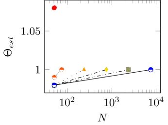
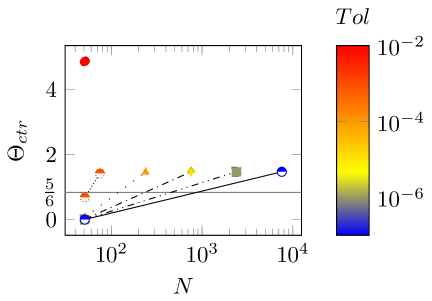
The overall algorithm performs also well when adaptive spatial refinement is used, as can be seen from Table 5. The quality of the estimation process is again very good, which leads to a significant reduction of the number of mesh points compared with the uniform approach. We have used $C_{\alpha}=10$ in the first two runs and $C_{\alpha}=100$ in the other ones to set $Tol^{\alpha}=C_{\alpha}\,Tol$ at the beginning. The number of adaptive grid points at the final time $T$ is denoted by $N_{M}$. After adjusting the spatial meshes until $A_{n}\leq Tol_{n}^{\alpha}=Tol^{\alpha}(1+\|V_{h,n}\|)$ holds, no further runs with higher tolerances in time are necessary. The evolution of the indicators $\Theta_{est}$ and $\Theta_{ctr}$ is visualized in Fig. 3.

Figure 3: Evolution of the efficiency indicators $\Theta_{est}$ (left) and $\Theta_{ctr}$ (right) for the Burgers problem, global tolerances $GTol=10^{-i},\,i=2,\ldots,4$, and adaptive refinement in space. Here, $Tol^{\alpha}$ is the local spatial tolerance. Different icons represent different $GTols$. The progress in the local time tolerance $Tol$ is described by diverse colouring. Control of the true global error, i.e. $\Theta_{ctr}\geq 5/6$, is achieved in all cases. Except for $GTol=10^{-3}$ and $Tol^{\alpha}=10^{-2}$, a second run is necessary for all global tolerances, indicated by connected icons. The quality of the estimates is very high.

Figure 4: Temporal evolution of the numerical solution for the Burgers’ problem with $Tol=10^{-3}$ and $51$ uniform grid points (left) and adaptive spatial refinement with $45$ grid points at the final time (right).

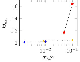
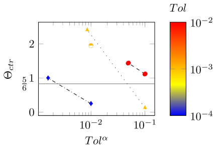
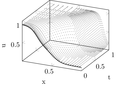
The numerical solutions obtained with $Tol=10^{-3}$ and $51$ uniform grid points (left) and adaptive spatial refinement with $45$ grid points at the final time (right) are plotted in Fig. 4. With less grid points, the adaptive scheme reduces the global error by nearly a factor $3$.

$Tol$	$N$	$Tol_{M}$	$\|\tilde{E}_{h,M}\|$	$\|{\tilde{e}}_{h,M}\|$	$\|{\tilde{\eta}}_{h,M}\|$	$\Theta_{est}$	$\Theta_{ctr}$	$q_{num}$
1.00e-2	103	2.05e-2	1.84e-0	1.45e-1	1.98e-0	9.89	0.11
4.69e-4	103	2.05e-2	5.78e-1	1.26e-3	5.79e-1	2.69	0.10
4.69e-4	677	2.02e-2	6.04e-3	1.11e-3	7.15e-3	1.19	3.98	2.34
1.00e-2	415	2.02e-2	7.69e-2	1.44e-1	6.73e-2	3.05	0.80
4.66e-4	415	2.02e-2	1.86e-2	1.11e-3	1.97e-2	1.23	1.34
4.66e-4	207	2.03e-2	9.17e-2	1.15e-3	9.29e-2	1.47	0.32	2.24
1.00e-3	207	2.03e-3	9.82e-2	2.97e-3	1.01e-1	1.60	0.03
2.27e-4	207	2.03e-3	8.80e-2	4.93e-4	8.85e-2	1.39	0.03
2.27e-4	1683	2.02e-3	6.14e-4	4.71e-4	1.09e-3	1.11	3.67	2.10
1.00e-3	831	2.02e-3	2.26e-3	2.87e-3	5.12e-3	1.33	1.19
2.35e-4	831	2.02e-3	4.01e-3	4.91e-4	4.50e-3	1.12	0.57
2.35e-4	1521	2.02e-3	8.42e-4	4.90e-4	1.33e-3	1.12	2.68	2.02
1.00e-4	1663	2.02e-4	8.89e-4	1.86e-4	1.08e-3	1.07	0.24
3.63e-5	1663	2.02e-4	9.88e-4	6.14e-5	1.05e-3	1.05	0.21
3.63e-5	4643	2.02e-4	7.30e-5	6.14e-5	1.34e-4	1.04	2.89	2.00

Table 6: Selected data for the Allen-Cahn problem. Uniform refinement in space is used.

$Tol$	$Tol^{\alpha}$	$N_{M}$	$Tol_{M}$	$\|\tilde{E}_{h,M}\|$	$\|{\tilde{e}}_{h,M}\|$	$\|{\tilde{\eta}}_{h,M}\|$	$\Theta_{est}$	$\Theta_{ctr}$
1.00e-2	1.00e-1	245	2.01e-2	1.05e-1	1.39e-1	3.42e-2	3.21	0.61
4.81e-4	1.00e-1	247	2.01e-2	8.54e-3	1.13e-3	9.67e-3	1.26	2.98
1.00e-3	1.00e-2	483	2.01e-3	1.26e-3	2.86e-3	1.59e-3	1.26	2.01
2.35e-4	1.00e-2	481	2.01e-3	9.72e-4	4.84e-4	1.46e-3	1.11	2.30
1.00e-4	1.00e-3	1839	2.01e-4	9.08e-5	1.85e-4	9.45e-5	1.63	3.62
3.62e-5	1.00e-3	1839	2.01e-4	5.49e-5	6.06e-5	1.16e-4	0.92	3.36
1.00e-4	1.00e-2	481	2.01e-4	1.23e-3	1.85e-4	1.41e-3	1.08	0.18
3.62e-5	1.00e-2	483	2.01e-4	1.32e-3	6.09e-5	1.38e-3	1.06	0.16
3.62e-5	9.68e-4	1839	2.01e-4	5.48e-5	6.07e-5	1.15e-4	0.92	3.36
1.00e-4	1.00e-1	243	2.01e-4	8.66e-3	1.84e-4	8.84e-3	1.15	0.03
3.62e-5	1.00e-1	243	2.01e-4	8.55e-3	6.08e-5	8.61e-3	1.12	0.03
3.62e-5	1.55e-3	1809	2.01e-4	5.68e-5	6.06e-5	1.17e-4	0.92	3.25

Table 7: Selected data for the Allen-Cahn problem. Adaptive refinement in space is used.

7.3 The Allen-Cahn equation

The third problem is the bi-stable Allen-Cahn equation which is defined by

$$\partial_{t}u=10^{-2}\,\partial_{xx}u+100u\,(1-u^{2})\,,\quad 0<x<2.5\,,\qquad 0<t\leq T=0.5\,,$$ (56)

with the initial function and Dirichlet boundary values taken from the exact wave front solution $u(x,t)=(1+e^{\lambda\,(x-\alpha\,t)})^{-1},\,\lambda=50\,\sqrt{2},\,\alpha=1.5\,\sqrt{2}$. This problem was also used in [2, 5].

First we apply uniform refinement in space. Table 6 reveals a high quality of the global error estimation and also the control process works quite well. Let us pick one exemplary run out to explain the overall control strategy in more detail. Starting with $GTol=Tol=10^{-3}$ and $831$ mesh points, which corresponds to the fourth simulation, the numerical scheme delivers global error estimates $\|{\tilde{e}}_{h,M}\|=2.87\times 10^{-3}$ and $\|{\tilde{\eta}}_{h,M}\|=5.12\times 10^{-3}$ for the time and spatial error of the approximate solution $V_{h,M}$ at the final time $t_{M}=T$. The first check for the time error estimate $\|{\tilde{e}}_{h,M}\|\leq C_{T}C_{control}Tol_{M}=8.08\times 10^{-4}$ fails and we adjust the local tolerances by a factor $fac=C_{T}Tol_{M}/\|{\tilde{e}}_{h,M}\|=2.35\times 10^{-1}$, which yields the new $Tol=2.35\,10^{-4}$. The computation is then redone. Due to the tolerance proportionality, in the second run the time error is significantly reduced and the inequality $\|{\tilde{e}}_{h,M}\|\leq 8.08\times 10^{-4}$ is now valid. We proceed with checking $\|\tilde{E}_{h,M}\|\leq C_{control}Tol_{M}=2.42\times 10^{-3}$, which is still not true. From (44), we compute a new number of spatial mesh points $N=1521$. Finally, the third run is successful and with the numerically observed spatial order $q_{num}=2.02$ the numerical solution is accepted.

Figure 5: Evolution of the efficiency indicators $\Theta_{est}$ (left) and $\Theta_{ctr}$ (right) for the Allen-Cahn problem, global tolerances $GTol=10^{-i},\,i=2,\ldots,4$, and uniform refinement in space. Different icons represent different $GTols$. The progress in the local time tolerance $Tol$ is described by diverse colouring. Control of the true global error, i.e. $\Theta_{ctr}\geq 5/6$, is achieved in all cases. An improvement of the spatial meshes is necessary for all global tolerances, indicated by connected icons. The quality of the estimates is very high after the control runs.

Figure 6: Evolution of the efficiency indicators $\Theta_{est}$ (left) and $\Theta_{ctr}$ (right) for the Allen-Cahn problem, global tolerances $GTol=10^{-i},\,i=2,\ldots,4$, and adaptive refinement in space. Here, $Tol^{\alpha}$ is the local spatial tolerance. Different icons represent different $GTols$. The progress in the local time tolerance $Tol$ is described by diverse colouring. Control of the true global error, i.e. $\Theta_{ctr}\geq 5/6$, is achieved in all cases. The quality of the estimates is very high.

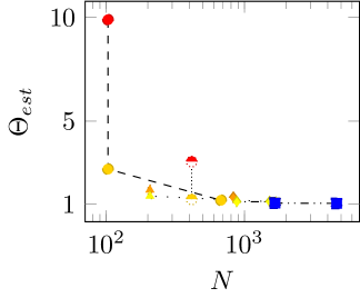
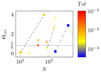
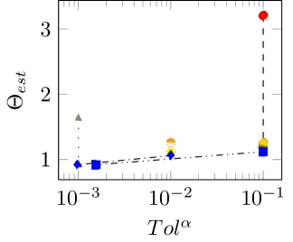
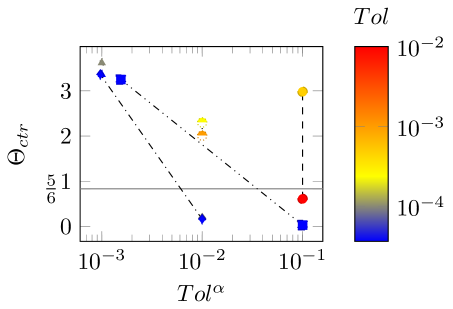
The ratios for $\Theta_{est}=\|\tilde{E}_{h,M}\|/\|E_{h}(T)\|$ in Table 6 lie between 1.04 and 1.23, after the control runs. Control of the global error, that is $\|E_{h}(T)\|\leq C_{control}Tol_{M}$, is in general achieved after two steps (one step to adjust the time grid and one step to control the spatial discretization), whereas the efficiency index $\Theta_{ctr}=Tol_{M}/\|E_{h}(T)\|$ is close to three. This results from a systematic cancellation effect between the global time and spatial error, which is not taken into account when computing $h_{new}$ from (44). The evolution of the indicators $\Theta_{est}$ and $\Theta_{ctr}$ is visualized in Fig. 5.

Figure 7: Temporal evolution of the numerical solution for the Allen-Cahn problem with $Tol=10^{-2}$ and $415$ uniform grid points (left) and adaptive spatial refinement with $245$ grid points at the final time (right).

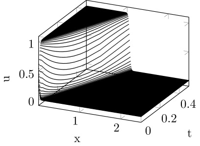
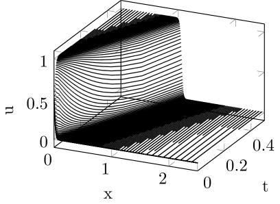
Next we consider locally adaptive spatial grid enhancement instead of globally uniform adaptation. Within each time step the grid is adapted by refinement and coarsening, based on an equidistribution principle, until $A_{n}\leq Tol_{n}^{\alpha}=Tol^{\alpha}(1+\|V_{h,n}\|)$ holds. This yields a sequence of non-uniform meshes. Let $N_{M}$ denote the number of adaptive grid points obtained at the final time $T$. The first three runs in Table 7 correspond to our standard setting $C_{\alpha}=10$, i.e., $Tol^{\alpha}=10\,Tol$. In this case, after adjusting the local tolerances for the time integration no further run with higher tolerances in space is necessary. To demonstrate the robustness of the algorithm, we select two additional runs with $C_{\alpha}=10^{l},l=2,3$, for $GTol=10^{-4}$. In both cases, coarser meshes are used at the beginning and a second control run has to be done to decrease the spatial discretization error. The resulting adaptive spatial meshes are comparable. Control of the global error is always achieved. The estimation process works again quite well. The evolution of the indicators $\Theta_{est}$ and $\Theta_{ctr}$ is visualized in Fig. 6. Compared to the uniform case, significantly less spatial degrees of freedoms are needed to reach the desired tolerances. The reduction rate varies between 40% and 70%. In Fig. 7 we have plotted the numerical solutions obtained with $Tol=10^{-2}$ and $415$ uniform grid points (left) and adaptive spatial refinement with $245$ grid points at the final time (right). The accuracies are comparable.

8 Summary

We have developed an error control strategy for finite difference solutions of parabolic equations, involving both temporal and spatial discretization errors. The global time error strategy discussed in [5] appears to provide an excellent starting point for the development of such an algorithm. The classical ODE approach used there and the principle of tolerance proportionality are combined with an efficient estimation of the spatial error and mesh adaptation to control the overall global error. Two approaches have been presented to handle spatial mesh improvement: (i) globally uniform refinement and (ii) local refinement and coarsening based on an equidistribution principle. Inspired by [1], we have used Richardson extrapolation to approximate the spatial truncation error within the method of lines. Our control strategy aims at balancing the spatial and temporal discretization error in order to achieve an accuracy imposed by the user.

The key ingredients are: (i) linearized error transport equations equipped with sufficiently accurate defects to approximate the global time error and global spatial error and (ii) uniform or adaptive mesh refinement and local error control in time based on tolerance proportionality to achieve global error control. For illustration of the performance and effectiveness of our approach, we have implemented second-order finite differences in one space dimension and the example integrator ROS3P [4]. On the basis of three different test problems we could observe that our approach is very reliable, both with respect to estimation and control.

Needless to say that spatial mesh adaptation locally in time is more efficient for solutions having a strongly nonuniform nature in space, especially if it varies over time. This is clearly visible for the travelling wave solution of the Allen-Cahn problem. However, optimized uniform strategies might also be of interest if users would like to extend their own software packages not having the option of dynamic adaptive mesh refinement to global error control.

References

- [1] M. Berzins (1988), Global error estimation in the method of lines for parabolic equations, SIAM J. Sci. Stat. Comput. 9, pp. 687-703.
- [2] K. Debrabant, J. Lang (2013), On global error estimation and control of finite difference solutions for parabolic equations, Adaptive Modeling and Simulation 2013 - Proceedings of the 6th International Conference on Adaptive Modeling and Simulation, ADMOS 2013, pp. 187-198.
- [3] J. Lang (2000), Adaptive Multilevel Solution of Nonlinear Parabolic PDE Systems. Theory, Algorithm and Applications, Lecture Notes in Computational Science and Engineering, Vol. 16, Springer.
- [4] J. Lang, J.G. Verwer (2001), ROS3P – An accurate third-order Rosenbrock solver designed for parabolic problems, BIT 41, pp. 731-738.
- [5] J. Lang, J.G. Verwer (2007), On global error estimation and control for initial value problems, SIAM J. Sci. Comput. 29, pp. 1460-1475.
- [6] S. Larsson, V. Thomée (2005), Partial Differential Equations with Numerical Methods, Texts in Applied Mathematics, Vol. 45, 2nd printing, Springer.
- [7] L. Lawson, M. Berzins, P.M. Dew (1991), Balancing space and time errors in the method of lines for parabolic equations, SIAM J. Sci. Stat. Comput. 12, pp. 573-594.
- [8] U. Nowak (1996), A fully adaptive MOL-treatment of parabolic 1D-problems with extrapolation techniques, Appl. Num. Math. 20, pp. 129-145.
- [9] M. Schmich, B. Vexler (2008), Adaptivity with dynamic meshes for space-time finite element discretizations of parabolic equations, SIAM J. Sci. Stat. Comput. 30, pp. 369-393.
- [10] W. Schönauer, E. Schnepf, K. Raith (1984), Experiences in designing P.D.E. software with selfadaptive variable step size/order difference methods, Computing 5, pp. 227-242.
- [11] L.F. Shampine (1994), Numerical Solution of Ordinary Differential Equations, Chapman & Hall, New York.
- [12] R.D. Skeel (1986), Thirteen ways to estimate global error, Numer. Math. 48, pp. 1-20.
- [13] J.W. Thomas (1995), Numerical Partial Differential Equations. Finite Difference Methods, Texts in Applied Mathematics 22, Springer.
- [14] A. Vande Wouver, P. Saucez, W.E. Schiesser (1998), Some user-oriented comparisons of adaptive grid methods for partial differential equations in one space dimension, Appl. Numer. Math. 26, pp. 49-62.
- [15] A. Vande Wouver, P. Saucez, W.E. Schiesser, S. Thompson (2005), A MATLAB implementation of upwind finite differences and adaptive grids in the method of lines, J. Comput. Appl. Math. 183, pp. 245-258.