FTUV/09-1111

IFIC/09-53

LPT-Orsay-09-90

Hadron structure in $\tau\rightarrow KK\pi\nu_{\tau}$ decays

D. Gómez Dumm¹, P. Roig², A. Pich³, J. Portolés³

¹⁾ IFLP, CONICET $-$ Dpto. de Física, Universidad Nacional de La Plata,

C.C. 67, 1900 La Plata, Argentina

²⁾ Laboratoire de Physique Théorique (UMR 8627), Université de Paris-Sud XI,

Bâtiment 210, 91405 Orsay cedex, France

³⁾ Departament de Física Teòrica, IFIC, CSIC — Universitat de València,

Edifici d’Instituts de Paterna, Apt. Correus 22085, E-46071 València, Spain

We analyse the hadronization structure of both vector and axial-vector currents leading to $\tau\to KK\pi\,\nu_{\tau}$ decays. At leading order in the $1/N_{C}$ expansion, and considering only the contribution of the lightest resonances, we work out, within the framework of the resonance chiral Lagrangian, the structure of the local vertices involved in those processes. The couplings in the resonance theory are constrained by imposing the asymptotic behaviour of vector and axial-vector spectral functions ruled by QCD. In this way we predict the hadron spectra and conclude that, contrarily to previous assertions, the vector contribution dominates by far over the axial-vector one in all $KK\pi$ charge channels.

PACS : 11.15.Pg, 12.38.-t, 12.39.Fe
      Keywords : Hadron tau decays, chiral Lagrangians, QCD, $1/N$ expansion.

1 Introduction

Hadron decays of the tau lepton provide a prime scenario to study the hadronization of QCD currents in an energy region settled by many resonances. This task has a twofold significance. First, the study of branching fractions and spectra of those decays is a major goal of the asymmetric B factories (BABAR, BELLE). These are supplying an enormous amount of quality data owing to their large statistics, and the same is planned for the near future at tau-charm factories such as BES-III. Second, the required hadronization procedures involve QCD in a non-perturbative energy region ($E\stackrel{{\scriptstyle<}}{{{}_{\sim}}}M_{\tau}\sim 1.8\,\mbox{GeV}$) and, consequently, these processes are a clean benchmark, not spoiled by an initial hadron state, where we can learn about the treatment of strong interactions when driven by resonances.

Analyses of tau decay data involve matrix elements that convey the hadronization of the vector and axial-vector currents. At present there is no determination from first principles of those matrix elements as they involve strong interaction effects in its non-perturbative regime. Therefore we have to rely in models that parameterize the form factors that arise from the hadronization. A relevant one is the so-called Kühn-Santamaría model (KS) [1] that, essentially, relies on the construction of form factors in terms of Breit-Wigner functions weighted by unknown parameters that are extracted from phenomenological analyses of data. This procedure, that has proven to be successful in the description of the $\pi\pi\pi$ final state, has been employed in the study of many two- and three-hadron tau decays [2, 3, 4, 5]. The ambiguity related with the choice of Breit-Wigner functions [1, 6] is currently being exploited to estimate the errors in the determination of the free parameters. The measurement of the $KK\pi$ spectrum by the CLEO Collaboration [7] has shown that the parameterization described by the KS model does not recall appropriately the experimental features keeping, at the same time, a consistency with the underlying strong interaction theory [8]. The solution provided by CLEO based in the introduction of new parameters spoils the normalization of the Wess-Zumino anomaly, i.e. a specific prediction of QCD. Indeed, arbitrary parameterizations are of little help in the procedure of obtaining information about non-perturbative QCD. They may fit the data but do not provide us hints on the hadronization procedures. The key point in order to uncover the inner structure of hadronization is to guide the construction of the relevant form factors with the use of known properties of QCD.

The TAUOLA library [9] is, at present, a key tool that handles analyses of tau decay data. Though originally it comprehended assorted versions of the KS model only, it has been opened to the introduction of matrix elements obtained with other models. Hence it has become an excellent tool where theoretical models confront experimental data. This or analogous libraries are appropriate benchmarks where to apply the results of our research.

At very low energies ($E\ll M_{\rho}$, being $M_{\rho}$ the mass of the $\rho(770)$ resonance) the chiral symmetry of massless QCD rules the construction of an effective field theory that allows a perturbative expansion in momenta ($p$) and light quark masses ($m$), as $(p^{2},M_{\pi}^{2})/\Lambda_{\chi}^{2}$, being $\Lambda_{\chi}\sim 4\pi F\sim M_{\rho}$ the scale that breaks the chiral symmetry; here $M_{\pi}$ is the pion mass and $F$ is the decay constant of the pion. Indeed Chiral Perturbation Theory ($\chi PT$) [10] drives the hadronization of QCD currents into the lightest multiplet of pseudoscalar mesons, $\pi$, $K$ and $\eta$. The application of this framework to the study of pion decays of the tau lepton was carried out in Ref. [11] though, obviously, it can only describe a tiny region of the available phase space. It is clear that, whatever the structure given to the form factors in the region of resonances, it should match the chiral constraint in its energy domain. In fact the parameterizations with Breit-Wigner functions that are at the center of the KS model fail to fulfill that condition already at ${\cal O}(p^{4})$ in the chiral expansion [12, 13].

Our knowledge of QCD in the energy region of the resonances is pretty poor. Contrarily to the very low energy domain, we do not know how to construct a dual effective field theory of strong interactions for $E\sim M_{\rho}$. There is a tool, though, that could shed light on the appropriate structure of a Lagrangian theory that we could use. This is yielded by the large-$N_{C}$ limit of $SU(N_{C})$ QCD [14], which introduces an expansion in inverse powers of the number of colours $N_{C}$. The essential idea relevant for our goal that comes out from that setting is that at leading order in the expansion, i.e. $N_{C}\rightarrow\infty$, any amplitude is given by the tree level diagrams generated by a local Lagrangian with an spectrum of infinite zero-width states. This frame, as we will see, can be used to establish a starting point in the study of the hadron resonance region and, consequently, in the hadron decays of the tau lepton. The setting recalls the role of the resonance chiral theory [15, 16] that can be better understood in the light of the large-$N_{C}$ limit [17, 18, 19].

At high energies ($E\gg M_{\rho}$), where the light-flavoured continuum is reached, perturbative QCD is the appropriate framework to deal with the description of strong interaction of partons. In particular, a well known feature of form factors of QCD currents is their smooth behaviour at high transfer of momenta [20], thus it is reasonable to expect that the form factors match this behaviour above the energy region of the resonances. Another related tool is the study of the Operator Product Expansion (OPE) of Green functions of QCD currents that are order parameters of the chiral symmetry breaking. It is possible to evaluate these Green functions within a resonance theory, and then perform a matching with their leading term of the OPE expansion at high transfers of momenta [21, 22, 23, 24, 25, 26, 27]. In general, the information coming from high energies is important to settle a resonance Lagrangian. It is reasonable to assume that the effective couplings collect information coming from the energy region above the resonances, hence the described procedure should help to determine the corresponding coupling constants. Indeed, this approach has proven to be capable of that task [27].

In Ref. [13] we considered all mentioned steps in order to analyse the $\pi\pi\pi$ hadron final state in the decay of the tau lepton. Here we continue that undertaking by considering the $KK\pi$ channels that, as mentioned above, do not fit well within the KS model and the present TAUOLA setup. Contrarily to the $\pi\pi\pi$ final state, which is dominated by the hadronization of the axial-vector current, $\tau\to KK\pi\nu_{\tau}$ decays receive contributions from both vector and axial-vector currents. Indeed, one of the goals of our work is to find out the relative weight of those contributions. Fortunately we will be assisted in this task by the recent analysis of $e^{+}e^{-}\rightarrow KK\pi$ cross-section by BABAR [28] where a separation between isoscalar and isovector channels has been performed. Hence we will be able to connect both processes through CVC.

In Section 2 we introduce the observables to be considered and the framework settled by the procedure sketched above. Then the amplitudes for $KK\pi$ decay channels are evaluated in Section 3. An analysis of how we can get information on the resonance couplings appearing in the hadronization of the currents is performed in Section 4. Finally we explain our results in Section 5, and our conclusions are pointed out in Section 6. Four technical appendices complete our exposition.

2 Theoretical framework

The hadronization of the currents that rule semileptonic tau decays is driven by non-perturbative QCD. As mentioned in the Introduction, our methodology stands on the construction of an action, with the relevant degrees of freedom, led by the chiral symmetry and the known asymptotic behaviour of form factors and Green functions driven by large $N_{C}$ QCD. We will limit ourselves to those pieces of the action that are relevant for the study of decays of the tau lepton into three pseudoscalar mesons. Hence we will need to include both even- and odd-intrinsic parity sectors.

The large $N_{C}$ expansion of $SU(N_{C})$ QCD implies that, in the $N_{C}\rightarrow\infty$ limit, the study of Green functions of QCD currents can be carried out through the tree level diagrams of a Lagrangian theory that includes an infinite spectrum of non-decaying states [14]. Hence the study of the resonance energy region can be performed by constructing such a Lagrangian theory. The problem is that we do not know how to implement an infinite spectrum in a model-independent way. However, it is well known from the phenomenology that the main role is always played by the lightest resonances. Accordingly it was suggested in Refs. [15, 16] that one can construct a suitable effective Lagrangian involving the lightest nonets of resonances and the octet of Goldstone bosons states ($\pi$, $K$ and $\eta$). This is indeed an appropriate tool to handle the hadron decays of the tau lepton. The guiding principle in the construction of such a Lagrangian is chiral symmetry. When resonances are integrated out from the theory, i.e. one tries to describe the energy region below such states ($E\ll M_{\rho}$), the remaining setting is that of $\chi$PT, to which now we turn.

The very low-energy strong interaction in the light quark sector is known to be ruled by the $SU(3)_{L}\otimes SU(3)_{R}$ chiral symmetry of massless QCD implemented in $\chi$PT. The leading even-intrinsic-parity ${\cal O}(p^{2})$ Lagrangian, which carries the information of the spontaneous symmetry breaking of the theory, is :

$${\cal L}_{\chi{\rm PT}}^{(2)}=\frac{F^{2}}{4}\langle u_{\mu}u^{\mu}+\chi_{+}\rangle\ ,$$ (1)

where

$$u_{\mu} = i[u^{\dagger}(\partial_{\mu}-ir_{\mu})u-u(\partial_{\mu}-i\ell_{\mu})u^{\dagger}]\ ,$$

$$\chi_{\pm} = u^{\dagger}\chi u^{\dagger}\pm u\chi^{\dagger}u\ \ \ \ ,\ \ \ \ \chi=2B_{0}(s+ip)\;\;,$$ (2)

and $\langle\ldots\rangle$ is short for a trace in the flavour space. The Goldstone octet of pseudoscalar fields

$$\Phi(x)=\left(\begin{array}[]{ccc}\displaystyle\frac{1}{\sqrt{2}}\,\pi^{0}+\displaystyle\frac{1}{\sqrt{6}}\,\eta_{8}&\pi^{+}&K^{+}\\ \pi^{-}&-\displaystyle\frac{1}{\sqrt{2}}\,\pi^{0}+\displaystyle\frac{1}{\sqrt{6}}\,\eta_{8}&K^{0}\\ K^{-}&\bar{K}^{0}&-\displaystyle\frac{2}{\sqrt{6}}\,\eta_{8}\end{array}\right)\ ,$$ (3)

is realized non–linearly into the unitary matrix in the flavour space

$$u(\varphi)=\exp\left\{\frac{i}{\sqrt{2}\,F}\Phi(x)\right\}\;\;\;,$$ (4)

which under chiral rotations transforms as

$$u(\varphi)\to g_{R}\,u(\varphi)\,h(g,\varphi)^{\dagger}=h(g,\varphi)\,u(\varphi)\,g_{L}^{\dagger}\;\;,$$ (5)

with $g\equiv(g_{L},g_{R})\,\in\,SU(3)_{\mathrm{L}}\otimes SU(3)_{\mathrm{R}}$ and $h(g,\varphi)\,\in\,SU(3)_{V}$. External hermitian matrix fields $r_{\mu}$, $\ell_{\mu}$, $s$ and $p$ promote the global $SU(3)_{\mathrm{L}}\otimes SU(3)_{\mathrm{R}}$ symmetry to a local one. Thus, interactions with electroweak bosons can be accommodated through the vector $v_{\mu}=(r_{\mu}+\ell_{\mu})/2$ and axial–vector $a_{\mu}=(r_{\mu}-\ell_{\mu})/2$ fields. The scalar field $s$ incorporates explicit chiral symmetry breaking through the quark masses taking $s={\cal M}\,+\ldots$, with ${\cal M}=\mathrm{diag}(m_{u},m_{d},m_{s})$ and, finally, at lowest order in the chiral expansion $F=F_{\pi}=92.4$ MeV is the pion decay constant and $B_{0}F^{2}=-\langle 0|\bar{\psi}\psi|0\rangle_{0}$.

The leading action in the odd-intrinsic-parity sector arises at ${\cal O}(p^{4})$. This is given by the chiral anomaly [29] and explicitly stated by the Wess-Zumino-Witten ${\cal Z}_{WZ}[v,a]$ functional that can be read in Ref. [30]. This contains all anomalous contributions to electromagnetic and semileptonic meson decays.

It is well known [15, 19] that higher orders in the chiral expansion, i.e. even-intrinsic-parity ${\cal L}_{\chi PT}^{(n)}$ with $n>2$, bring in the information of heavier degrees of freedom that have been integrated out, for instance resonance states. As our next step intends to include the latter explicitly, to avoid double counting issues we will not consider higher orders in $\chi$PT. As we comment below, in order to fulfill this procedure —at least, up to ${\cal O}(p^{4})$— it is convenient to use the antisymmetric tensor representation for the $J=1$ fields. Analogously, additional odd-intrinsic-parity amplitudes arise at ${\cal O}(p^{6})$ in $\chi$PT, either from one-loop diagrams using one vertex from the Wess-Zumino-Witten action or from tree-level operators [31]. However we will assume that the latter are fully generated by resonance contributions [24] and, therefore, will not be included in the following.

The formulation of a Lagrangian theory that includes both the octet of Goldstone mesons and $U(3)$ nonets of resonances is carried out through the construction of a phenomenological Lagrangian [32] where chiral symmetry determines the structure of the operators. Given the vector character of the Standard Model (SM) couplings of the hadron matrix elements in $\tau$ decays, form factors for these processes are ruled by vector and axial-vector resonances. Notwithstanding those form factors are given, in the $\tau\rightarrow PPP\nu_{\tau}$ decays, by a four-point Green function where other quantum numbers might play a role, namely scalar and pseudoscalar resonances [33]. However their contribution should be minor for $\tau\rightarrow KK\pi\nu_{\tau}$. Indeed the lightest scalar, namely $f_{0}(980)$, couples dominantly to two pions, and therefore its role in the $K\overline{K}\pi$ final state should be negligible. Heavier flavoured or unflavoured scalars and pseudoscalars are at least suppressed by their masses, being heavier than the axial-vector meson $a_{1}(1260)$ (like $K_{0}^{*}(1430)$ that couples to $K\pi$). In addition the couplings of unflavoured states to $K\overline{K}$ (scalars) and $K\overline{K}\pi$ (pseudoscalars) seem to be very small [35]. Thus in our description we include $J=1$ resonances only , and this is done by considering a nonet of fields [15] :

$$R\,\equiv\,\frac{1}{\sqrt{2}}\,\sum_{i=1}^{9}\lambda_{i}\,\phi_{R,i}\;,$$ (6)

where $R=V,A$, stands for vector and axial-vector resonance states. Under the $SU(3)_{L}\otimes SU(3)_{R}$ chiral group, $R$ transforms as :

$$R\,\rightarrow\,h(g,\varphi)\,R\,h(g,\varphi)^{\dagger}\;.$$ (7)

The flavour structure of the resonances is analogous to that of the Goldstone bosons in Eq. (3). We also introduce the covariant derivative

$$\nabla_{\mu}X \equiv \partial_{\mu}X+[\Gamma_{\mu},X]\;\;,$$ (8)

$$\Gamma_{\mu} = \frac{1}{2}\,[\,u^{\dagger}(\partial_{\mu}-ir_{\mu})u+u(\partial_{\mu}-i\ell_{\mu})u^{\dagger}\,]\;\;,$$

acting on any object $X$ that transforms as $R$ in Eq. (7), like $u_{\mu}$ and $\chi_{\pm}$. The kinetic terms for the spin 1 resonances in the Lagrangian read :

$${\cal L}_{\rm kin}^{R}=-\frac{1}{2}\langle\,\nabla^{\lambda}R_{\lambda\mu}\nabla_{\nu}R^{\nu\mu}\,\rangle+\frac{M_{R}^{2}}{4}\,\langle\,R_{\mu\nu}R^{\mu\nu}\,\rangle\;\;\;,\;\;\;\;\;R\,=\,V,A\;,$$ (9)

$M_{V}$, $M_{A}$ being the masses of the nonets of vector and axial–vector resonances in the chiral and large-$N_{C}$ limits, respectively. Notice that we describe the resonance fields through the antisymmetric tensor representation. With this description one is able to collect, upon integration of resonances, the bulk of the low-energy couplings at ${\cal O}(p^{4})$ in $\chi$PT without the inclusion of additional local terms [27]. In fact it is necessary to use this representation if one does not include the ${\cal L}_{\chi PT}^{(4)}$ in the Lagrangian theory. Though analogous studies at higher chiral orders have not been carried out, we will assume that no ${\cal L}_{\chi PT}^{(n)}$ with $n=4,6,...$ in the even-intrinsic-parity and $n=6,8,...$ in the odd-intrinsic-parity sectors need to be included in the theory.

The construction of the interaction terms involving resonance and Goldstone fields is driven by chiral and discrete symmetries with a generic structure given by :

$${\cal O}_{i}\,\sim\,\langle\,R_{1}R_{2}...R_{j}\,\chi^{(n)}(\varphi)\,\rangle\,,$$ (10)

where $\chi^{(n)}(\varphi)$ is a chiral tensor that includes only Goldstone and auxiliary fields. It transforms like $R$ in Eq. (7) and has chiral counting $n$ in the frame of $\chi$PT. This counting is relevant in the setting of the theory because, though the resonance theory itself has no perturbative expansion, higher values of $n$ may originate violations of the proper asymptotic behaviour of form factors or Green functions. As a guide we will include at least those operators that, contributing to our processes, are leading when integrating out the resonances. In addition we do not include operators with higher-order chiral tensors, $\chi^{(n)}(\varphi)$, that would violate the QCD asymptotic behaviour unless their couplings are severely fine tuned to ensure the needed cancellations of large momenta. In the odd-intrinsic-parity sector, that gives the vector form factor, this amounts to include all $\langle R\chi^{(4)}\rangle$ and $\langle RR\chi^{(2)}\rangle$ terms. In the even-intrinsic-parity couplings, giving the axial-vector form factors, these are the terms $\langle R\chi^{(2)}\rangle$. However previous analyses of the axial-vector contributions [13, 23] show the relevant role of the $\langle RR\chi^{(2)}\rangle$ terms that, accordingly, are also considered here .

We also assume exact $SU(3)$ symmetry in the construction of the interacting terms, i.e. at level of couplings. Deviations from exact symmetry in hadronic tau decays have been considered in Ref. [34]. However we do not include $SU(3)$ breaking couplings because we are neither considering next-to-leading corrections in the $1/N_{C}$ expansion.

The lowest order interaction operators linear in the resonance fields have the structure $\langle R\chi^{(2)}(\varphi)\rangle$. There are no odd-intrinsic-parity terms of this form. The even-intrinsic-parity Lagrangian includes three coupling constants [15] :

$${\cal L}_{2}^{\mbox{\tiny V}} = \frac{F_{V}}{2\sqrt{2}}\langle V_{\mu\nu}f_{+}^{\mu\nu}\rangle+i\,\frac{G_{V}}{\sqrt{2}}\langle V_{\mu\nu}u^{\mu}u^{\nu}\rangle\;\,,$$

$${\cal L}_{2}^{\mbox{\tiny A}} = \frac{F_{A}}{2\sqrt{2}}\langle A_{\mu\nu}f_{-}^{\mu\nu}\rangle\;,$$ (11)

where $f_{\pm}^{\mu\nu}=uF_{L}^{\mu\nu}u^{\dagger}\pm u^{\dagger}F_{R}^{\mu\nu}u$ and $F_{R,L}^{\mu\nu}$ are the field strength tensors associated with the external right- and left-handed auxiliary fields. All coupling parameters $F_{V}$, $G_{V}$ and $F_{A}$ are real.

The leading odd-intrinsic-parity operators, linear in the resonance fields, have the form $\langle R\chi^{(4)}(\varphi)\rangle$. We will need those pieces that generate : i) the vertex with one vector resonance and three pseudoscalar fields; ii) the vertex with one vector resonance, a vector current and one pseudoscalar. The minimal Lagrangian with these features is :

$${\cal L}_{4}^{\mbox{\tiny V}}=\sum_{i=1}^{5}\,\frac{g_{i}}{M_{V}}\,{\cal O}^{i}_{\mbox{\tiny VPPP}}\;+\;\sum_{i=1}^{7}\,\frac{c_{i}}{M_{V}}\,{\cal O}^{i}_{\mbox{\tiny{VJP}}}\,,$$ (12)

where $g_{i}$ and $c_{i}$ are real adimensional couplings, and the operators read

• VPPP terms

  $${\cal O}_{\mbox{\tiny VPPP}}^{1} = i\,\varepsilon_{\mu\nu\alpha\beta}\,\left\langle V^{\mu\nu}\,\left(\,h^{\alpha\gamma}u_{\gamma}u^{\beta}-u^{\beta}u_{\gamma}h^{\alpha\gamma}\right)\right\rangle\,,$$

  $${\cal O}_{\mbox{\tiny VPPP}}^{2} = i\,\varepsilon_{\mu\nu\alpha\beta}\,\left\langle V^{\mu\nu}\,\left(\,h^{\alpha\gamma}u^{\beta}u_{\gamma}-u_{\gamma}u^{\beta}h^{\alpha\gamma}\,\right)\right\rangle\,,$$

  $${\cal O}_{\mbox{\tiny VPPP}}^{3} = i\,\varepsilon_{\mu\nu\alpha\beta}\,\left\langle V^{\mu\nu}\,\left(\,u_{\gamma}h^{\alpha\gamma}u^{\beta}-u^{\beta}h^{\alpha\gamma}u_{\gamma}\,\right)\right\rangle\,,$$

  $${\cal O}_{\mbox{\tiny VPPP}}^{4} = \varepsilon_{\mu\nu\alpha\beta}\,\left\langle\left\{\,V^{\mu\nu}\,,\,u^{\alpha}\,u^{\beta}\,\right\}\,{\cal\chi}_{-}\right\rangle\,,$$

  $${\cal O}_{\mbox{\tiny VPPP}}^{5} = \varepsilon_{\mu\nu\alpha\beta}\,\left\langle\,u^{\alpha}\,V^{\mu\nu}\,u^{\beta}\,{\cal\chi}_{-}\right\rangle\,,$$ (13)

  with $h_{\mu\nu}=\nabla_{\mu}u_{\nu}+\nabla_{\nu}u_{\mu}$, and

• VJP terms [24]

  $${\cal O}_{\mbox{\tiny VJP}}^{1} = \varepsilon_{\mu\nu\rho\sigma}\,\langle\,\{V^{\mu\nu},f_{+}^{\rho\alpha}\}\nabla_{\alpha}u^{\sigma}\,\rangle\;\;,$$

  $${\cal O}_{\mbox{\tiny VJP}}^{2} = \varepsilon_{\mu\nu\rho\sigma}\,\langle\,\{V^{\mu\alpha},f_{+}^{\rho\sigma}\}\nabla_{\alpha}u^{\nu}\,\rangle\;\;,$$

  $${\cal O}_{\mbox{\tiny VJP}}^{3} = i\,\varepsilon_{\mu\nu\rho\sigma}\,\langle\,\{V^{\mu\nu},f_{+}^{\rho\sigma}\}\,\chi_{-}\,\rangle\;\;,$$

  $${\cal O}_{\mbox{\tiny VJP}}^{4} = i\,\varepsilon_{\mu\nu\rho\sigma}\,\langle\,V^{\mu\nu}\,[\,f_{-}^{\rho\sigma},\chi_{+}]\,\rangle\;\;,$$

  $${\cal O}_{\mbox{\tiny VJP}}^{5} = \varepsilon_{\mu\nu\rho\sigma}\,\langle\,\{\nabla_{\alpha}V^{\mu\nu},f_{+}^{\rho\alpha}\}u^{\sigma}\,\rangle\;\;,$$

  $${\cal O}_{\mbox{\tiny VJP}}^{6} = \varepsilon_{\mu\nu\rho\sigma}\,\langle\,\{\nabla_{\alpha}V^{\mu\alpha},f_{+}^{\rho\sigma}\}u^{\nu}\,\rangle\;\;,$$

  $${\cal O}_{\mbox{\tiny VJP}}^{7} = \varepsilon_{\mu\nu\rho\sigma}\,\langle\,\{\nabla^{\sigma}V^{\mu\nu},f_{+}^{\rho\alpha}\}u_{\alpha}\,\rangle\;\;.$$ (14)

Notice that we do not include analogous pieces with an axial-vector resonance, that would contribute to the hadronization of the axial-vector current. This has been thoroughly studied in Ref. [13] (see also Ref. [37]) in the description of the $\tau\rightarrow\pi\pi\pi\nu_{\tau}$ process and it is shown that no $\langle A\chi^{(4)}(\varphi)\rangle$ operators are needed to describe its hadronization. Therefore those operators are not included in our minimal description of the relevant form factors.

In order to study tau decay processes with three pseudoscalar mesons in the final state one also has to consider non-linear terms in the resonance fields. Indeed the hadron final state in $\tau\rightarrow PPP\nu_{\tau}$ decays can be driven by vertices involving two resonances and a pseudoscalar meson. The structure of the operators that give those vertices is $\langle R_{1}R_{2}\chi^{(2)}(\varphi)\rangle$, and has been worked out before [13, 24]. They include both even- and odd-intrinsic-parity terms :

$${\cal L}_{2}^{\mbox{\tiny RR}}\,=\,\sum_{i=1}^{5}\,\lambda_{i}\,{\cal O}^{i}_{\mbox{\tiny VAP}}\;\;+\;\sum_{i=1}^{4}\,d_{i}\,{\cal O}^{i}_{\mbox{\tiny{VVP}}}\;,$$ (15)

where $\lambda_{i}$, and $d_{i}$ are unknown real adimensional couplings. The operators ${\cal O}^{i}_{\mbox{\tiny RRP}}$ are given by :

• VAP terms

  $${\cal O}^{1}_{\mbox{\tiny VAP}} = \langle\,[\,V^{\mu\nu}\,,\,A_{\mu\nu}\,]\,\chi_{-}\,\rangle\;\;,$$

  $${\cal O}^{2}_{\mbox{\tiny VAP}} = i\,\langle\,[\,V^{\mu\nu}\,,\,A_{\nu\alpha}\,]\,h_{\mu}^{\;\alpha}\,\rangle\;\;,$$ (16)

  $${\cal O}^{3}_{\mbox{\tiny VAP}} = i\,\langle\,[\,\nabla^{\mu}V_{\mu\nu}\,,\,A^{\nu\alpha}\,]\,u_{\alpha}\,\rangle\;\;,$$

  $${\cal O}^{4}_{\mbox{\tiny VAP}} = i\,\langle\,[\,\nabla^{\alpha}V_{\mu\nu}\,,\,A_{\alpha}^{\;\nu}\,]\,u^{\mu}\,\rangle\;\;,$$

  $${\cal O}^{5}_{\mbox{\tiny VAP}} = i\,\langle\,[\,\nabla^{\alpha}V_{\mu\nu}\,,\,A^{\mu\nu}\,]\,u_{\alpha}\,\rangle\;\;.$$

• VVP terms

  $${\cal O}_{\mbox{\tiny VVP}}^{1} = \varepsilon_{\mu\nu\rho\sigma}\,\langle\,\{V^{\mu\nu},V^{\rho\alpha}\}\nabla_{\alpha}u^{\sigma}\,\rangle\;\;,$$

  $${\cal O}_{\mbox{\tiny VVP}}^{2} = i\,\varepsilon_{\mu\nu\rho\sigma}\,\langle\,\{V^{\mu\nu},V^{\rho\sigma}\}\,\chi_{-}\,\rangle\;\;,$$

  $${\cal O}_{\mbox{\tiny VVP}}^{3} = \varepsilon_{\mu\nu\rho\sigma}\,\langle\,\{\nabla_{\alpha}V^{\mu\nu},V^{\rho\alpha}\}u^{\sigma}\,\rangle\;\;,$$

  $${\cal O}_{\mbox{\tiny VVP}}^{4} = \varepsilon_{\mu\nu\rho\sigma}\,\langle\,\{\nabla^{\sigma}V^{\mu\nu},V^{\rho\alpha}\}u_{\alpha}\,\rangle\;\;.$$ (17)

We emphasize that ${\cal L}_{2}^{\mbox{\tiny RR}}$ is a complete basis for constructing vertices with only one pseudoscalar meson; for a larger number of pseudoscalars additional operators might be added. As we are only interested in tree-level diagrams, the equation of motion arising from ${\cal L}_{\chi PT}^{(2)}$ in Eq. (1) has been used in ${\cal L}_{4}^{\mbox{\tiny V}}$ and ${\cal L}^{\mbox{\tiny RR}}_{2}$ to eliminate superfluous operators.

Hence our theory is given by the Lagrangian :

$${\cal L}_{R\chi T}\,=\,{\cal L}_{\chi PT}^{(2)}\,+\,{\cal L}_{\mbox{\tiny kin}}^{\mbox{\tiny R}}\,+\,{\cal L}_{2}^{\mbox{\tiny A}}\,+\,{\cal L}_{2}^{\mbox{\tiny V}}\,+\,{\cal L}_{4}^{\mbox{\tiny V}}\,+\,{\cal L}_{2}^{\mbox{\tiny RR}}\,.$$ (18)

It is important to point out that the resonance theory constructed above is not a theory of QCD for arbitrary values of the couplings in the interaction terms. As we will see later on, these constants can be constrained by imposing well accepted dynamical properties of the underlying theory.

3 Vector and axial-vector currents in $\tau\rightarrow KK\pi\,\nu_{\tau}$ decays

The decay amplitude for the $\tau\rightarrow KK\pi\nu_{\tau}$ decays can be written in the Standard Model as

$${\cal M}\,=\,-\,\frac{G_{F}}{\sqrt{2}}\,V_{ud}\,\overline{u}_{\nu_{\tau}}\,\gamma^{\mu}\left(1\,-\,\gamma_{5}\right)\,u_{\tau}\,T_{\mu}\;,$$ (19)

where $V_{ud}$ is an element of the Cabibbo-Kobayashi-Maskawa matrix and $T_{\mu}$ is the hadron matrix element of the participating $V_{\mu}-A_{\mu}$ QCD current :

$$T_{\mu}\,=\,\langle K(p_{1})\,K(p_{2})\,\pi(p_{3})\,|\,\left(V_{\mu}-A_{\mu}\right)e^{i{\cal L}_{QCD}}\,|\,0\rangle\,.$$ (20)

The hadron tensor can be written in terms of four form factors $F_{1}$, $F_{2}$, $F_{3}$ and $F_{4}$ as [36] :

$$T^{\mu}\,=\,V_{1}^{\mu}\,F_{1}\,+\,V_{2}^{\mu}\,F_{2}\,+\,V_{3}^{\mu}\,F_{3}\,+\,Q^{\mu}\,F_{4}\;,$$ (21)

where $Q^{\mu}=p_{1}^{\mu}+p_{2}^{\mu}+p_{3}^{\mu}$ and

$$V_{1\,\mu} = \left(\,g_{\mu\nu}-\frac{Q_{\mu}Q_{\nu}}{Q^{2}}\right)\,\left(p_{2}-p_{1}\right)^{\nu}\;,\;\;\;\;\;\;\;\;\;\;V_{2\,\mu}\;=\;\left(\,g_{\mu\nu}-\frac{Q_{\mu}Q_{\nu}}{Q^{2}}\right)\,\left(p_{3}-p_{1}\right)^{\nu}\,,$$

$$V_{3\,\mu} = i\,\varepsilon_{\mu\nu\varrho\sigma}\,p_{1}^{\nu}\,p_{2}^{\varrho}\,p_{3}^{\sigma}\;.$$ (22)

There are three different charge channels for the $KK\pi$ decays of the $\tau^{-}$ lepton, namely $K^{+}(p_{+})\,K^{-}(p_{-})\,\pi^{-}(p_{\pi})$, $K^{0}(p_{0})\,\overline{K}^{0}(\overline{p}_{0})\,\pi^{-}(p_{\pi})$ and $K^{-}(p_{-})\,K^{0}(p_{0})\,\pi^{0}(p_{\pi})$. The definitions of Eq. (3) correspond to the choice $p_{3}=p_{\pi}$ in all cases, and : $(p_{1},p_{2})=(p_{+},p_{-})$ for the $K^{+}\,K^{-}$ case, $(p_{1},p_{2})=(\overline{p}_{0},p_{0})$ for $K^{0}\,\overline{K}^{0}$ and $(p_{1},p_{2})=(p_{-},p_{0})$ for $K^{-}\,K^{0}$. In general, form factors $F_{i}$ are functions of the kinematical invariants : $Q^{2}$, $s=(p_{1}+p_{2})^{2}$ and $t=(p_{1}+p_{3})^{2}$. $F_{1}$ and $F_{2}$ originate from the axial-vector current, while $F_{3}$ follows from the vector current. All of them correspond to spin-1 transitions. The $F_{4}$ pseudoscalar form factor stems from the axial-vector current, and corresponds to a spin-0 transition. It is seen that this form factor vanishes in the chiral limit, therefore its contribution is expected to be heavily suppressed, and both the spectrum and the branching ratio of tau decays into three pseudoscalar mesons is dominated by $J=1$ transitions, especially in the Cabibbo-allowed modes.

The $Q^{2}$-spectrum is given by :

$$\frac{d\,\Gamma}{d\,Q^{2}}\,=\,\frac{G_{F}^{2}\,|V_{ud}|^{2}}{128\,(2\pi)^{5}\,M_{\tau}}\,\left(\frac{M_{\tau}^{2}}{Q^{2}}-1\right)^{2}\,\int\,ds\,dt\,\left[W_{SA}+\frac{1}{3}\left(1+2\frac{Q^{2}}{M_{\tau}^{2}}\right)\left(W_{A}+W_{B}\right)\right]\,,$$ (23)

where the hadron structure functions, introduced in Ref. [36], are :

$$W_{A} = -(V_{1}^{\mu}F_{1}+V_{2}^{\mu}F_{2})(V_{1\mu}F_{1}+V_{2\mu}F_{2})^{*}\,,$$

$$W_{B} = \frac{1}{4}\left[\,s\,t\,u\,+\,(m_{K}^{2}-m_{\pi}^{2})\,(Q^{2}-m_{K}^{2})\,s\,+\,m_{K}^{2}(2m_{\pi}^{2}-Q^{2})\,Q^{2}\ -\,m_{K}^{2}m_{\pi}^{4}\,\right]\,|F_{3}|^{2}\,,$$

$$W_{SA} = (Q^{\mu}\,F_{4})(Q_{\mu}F_{4}^{*})\,=\,Q^{2}\,|F_{4}|^{2}\,,$$ (24)

where $u=Q^{2}-s-t+2m_{K}^{2}+m_{\pi}^{2}$. The phase-space integrals extend over the region spanned by the hadron system with a center-of-mass energy $\sqrt{Q^{2}}$ :

$$\int\,ds\,dt\,\equiv\,\int_{4\,m_{K}^{2}}^{(\sqrt{Q^{2}}-m_{\pi})^{2}}ds\,\int_{t_{-}(s)}^{t_{+}(s)}dt\,,$$ (25)

with

$$t_{\pm}(s)\,=\,\frac{1}{4\,s}\left\{\left(Q^{2}-m_{\pi}^{2}\right)^{2}\,-\,\left[\lambda^{1/2}\left(Q^{2},s,m_{\pi}^{2}\right)\,\mp\,\lambda^{1/2}\left(m_{K}^{2},m_{K}^{2},s\right)\right]^{2}\right\}\,,$$ (26)

and $\lambda(a,b,c)=(a+b-c)^{2}-4ab$. We have neglected here the $\nu_{\tau}$ mass, and exact isospin symmetry has been assumed.

The general structure of the form factors, within our model, arises from the diagrams displayed in Fig. 1.

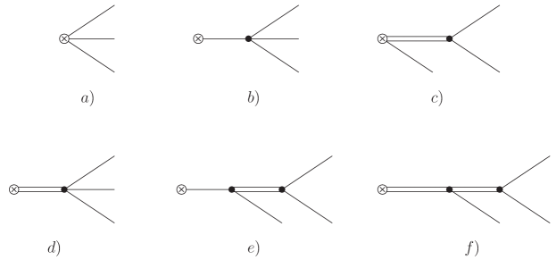
Figure 1: Topologies contributing to the final hadron state in $\tau\rightarrow KK\pi\,\nu_{\tau}$ decays in the $N_{C}\rightarrow\infty$ limit. A crossed circle indicates the QCD vector or axial-vector current insertion. A single line represents a pseudoscalar meson ($K$, $\pi$) while a double line stands for a resonance intermediate state. Topologies $b)$ and $e)$ only contribute to the axial-vector driven form factors, while diagram $d)$ arises only (as explained in the text) from the vector current.

This provides the following decomposition :

$$F_{i}\,=\,F_{i}^{\chi}\,+\,F_{i}^{\mbox{\tiny R}}\,+\,F_{i}^{\mbox{\tiny RR}}\;,\;\;\,i=1,...\,,$$ (27)

where $F_{i}^{\chi}$ is given by the $\chi$PT Lagrangian [topologies $a)$ and $b)$ in Fig. 1], and the rest are the contributions of one [Fig. 1$c)$, $d)$ and $e)$] or two resonances [Fig. 1$f)$].

3.1 Form factors in $\tau^{-}\rightarrow K^{+}K^{-}\,\pi^{-}\,\nu_{\tau}$ and $\tau^{-}\rightarrow K^{0}\,\overline{K^{0}}\,\pi^{-}\,\nu_{\tau}$

In the isospin limit, form factors for the $\tau^{-}\rightarrow K^{+}K^{-}\pi^{-}\nu_{\tau}$ and $\tau^{-}\rightarrow K^{0}\overline{K^{0}}\pi^{-}\nu_{\tau}$ decays are identical. The explicit expressions for these are :

$$F_{1}^{\chi} = -\frac{\sqrt{2}}{3\,F}\,,$$

$$F_{1}^{\mbox{\tiny R}}(s,t) = -\,\frac{\sqrt{2}}{6}\,\frac{F_{V}\,G_{V}}{F^{3}}\,\left[\,\frac{A^{\mbox{\tiny R}}(Q^{2},s,u,m_{K}^{2},m_{\pi}^{2},m_{K}^{2})}{M_{\rho}^{2}-s}\,+\,\frac{B^{\mbox{\tiny R}}(s,u,m_{K}^{2},m_{\pi}^{2})}{M_{K^{*}}^{2}-t}\,\right],\,$$ (28)

$$F_{1}^{\mbox{\tiny RR}}(s,t) = \frac{2}{3}\,\frac{F_{A}G_{V}}{F^{3}}\,\frac{Q^{2}}{M_{a_{1}}^{2}-Q^{2}}\,\,\left[\,\frac{A^{\mbox{\tiny RR}}(Q^{2},s,u,m_{K}^{2},m_{\pi}^{2},m_{K}^{2})}{M_{\rho}^{2}-s}\,\right.$$

$$\qquad\qquad\qquad\qquad\qquad\left.+\,\frac{B^{\mbox{\tiny RR}}(Q^{2},s,u,t,m_{K}^{2},m_{\pi}^{2},m_{K}^{2})}{M_{K^{*}}^{2}-t}\,\right]\,\,,$$

where the functions $A^{\mbox{\tiny R}}$, $B^{\mbox{\tiny R}}$, $A^{\mbox{\tiny RR}}$ and $B^{\mbox{\tiny RR}}$ are defined in Appendix A. The dependence of the form factors with $t$ follows from the relation $u=Q^{2}-s-t+2m_{K}^{2}+m_{\pi}^{2}$. Moreover resonance masses correspond to the lowest states, $M_{\rho}=M_{\rho(770)}$, $M_{K^{*}}=M_{K^{*}(892)}$ and $M_{a_{1}}=M_{a_{1}(1260)}$.

Analogously the $F_{2}$ form factor is given by :

$$F_{2}^{\chi} = F_{1}^{\chi}\,,$$

$$F_{2}^{\mbox{\tiny R}}(s,t) = -\,\frac{\sqrt{2}}{6}\,\frac{F_{V}\,G_{V}}{F^{3}}\,\left[\,\frac{B^{\mbox{\tiny R}}(t,u,m_{K}^{2},m_{K}^{2})}{M_{\rho}^{2}-s}\,+\,\frac{A^{\mbox{\tiny R}}(Q^{2},t,u,m_{K}^{2},m_{K}^{2},m_{\pi}^{2})}{M_{K^{*}}^{2}-t}\,\right],\,$$ (29)

$$F_{2}^{\mbox{\tiny RR}}(s,t) = \frac{2}{3}\,\frac{F_{A}G_{V}}{F^{3}}\,\frac{Q^{2}}{M_{a_{1}}^{2}-Q^{2}}\,\,\left[\,\frac{B^{\mbox{\tiny RR}}(Q^{2},t,u,s,m_{K}^{2},m_{K}^{2},m_{\pi}^{2})}{M_{\rho}^{2}-s}\,\right.$$

$$\qquad\qquad\qquad\qquad\qquad\left.+\,\frac{A^{\mbox{\tiny RR}}(Q^{2},t,u,m_{K}^{2},m_{K}^{2},m_{\pi}^{2})}{M_{K^{*}}^{2}-t}\,\right]\,\,.$$

The $F_{3}$ form factor arises from the chiral anomaly and the non-anomalous odd-intrinsic-parity amplitude. We obtain :

$$F_{3}^{\chi} = -\frac{N_{C}\,\sqrt{2}}{12\,\pi^{2}\,F^{3}}\,,$$

$$F_{3}^{\mbox{\tiny R}}(s,t) = -\frac{4\,G_{V}}{M_{V}\,F^{3}}\,\left[\,C^{\mbox{\tiny R}}(Q^{2},s,m_{K}^{2},m_{K}^{2},m_{\pi}^{2})\,\left(\sin^{2}\theta_{V}\frac{1+\sqrt{2}\cot\theta_{V}}{M_{\omega}^{2}-s}\right.\right.$$ (30)

$$\qquad\qquad\;\;\left.+\,\cos^{2}\theta_{V}\frac{1-\sqrt{2}\tan\theta_{V}}{M_{\phi}^{2}-s}\right)\,+\,\frac{C^{\mbox{\tiny R}}(Q^{2},t,m_{K}^{2},m_{\pi}^{2},m_{K}^{2})}{M_{K^{*}}^{2}-t}$$

$$\qquad\qquad\;\;\left.\,-\,\frac{2\,F_{V}}{G_{V}}\,\frac{D^{\mbox{\tiny R}}(Q^{2},s,t)}{M_{\rho}^{2}-Q^{2}}\right]\,,$$

$$F_{3}^{\mbox{\tiny RR}}(s,t) = 4\sqrt{2}\frac{F_{V}\,G_{V}}{F^{3}}\,\frac{1}{M_{\rho}^{2}-Q^{2}}\,\left[C^{\mbox{\tiny RR}}(Q^{2},s,m_{\pi}^{2})\,\left(\sin^{2}\theta_{V}\frac{1+\sqrt{2}\cot\theta_{V}}{M_{\omega}^{2}-s}\right.\right.$$

$$\qquad\qquad\qquad\qquad\qquad\;\left.\left.+\,\cos^{2}\theta_{V}\frac{1-\sqrt{2}\tan\theta_{V}}{M_{\phi}^{2}-s}\right)\,+\,\frac{C^{\mbox{\tiny RR}}(Q^{2},t,m_{K}^{2})}{M_{K^{*}}^{2}-t}\right]\,,$$

where $C^{\mbox{\tiny R}}$, $D^{\mbox{\tiny R}}$ and $C^{\mbox{\tiny RR}}$ are defined in Appendix A, and $\theta_{V}$ is the mixing angle between the octet and singlet vector states $\omega_{8}$ and $\omega_{0}$ that defines the mass eigenstates $\omega(782)$ and $\phi(1020)$ :

$$\left(\begin{array}[]{c}\phi\\ \omega\end{array}\right)\,=\,\left(\begin{array}[]{cc}\cos\theta_{V}&-\sin\theta_{V}\\ \sin\theta_{V}&\cos\theta_{V}\end{array}\right)\;\left(\begin{array}[]{c}\omega_{8}\\ \omega_{0}\end{array}\right)\,.$$ (31)

For numerical evaluations we will assume ideal mixing, i.e. $\theta_{V}=\tan^{-1}(1/\sqrt{2})$. In this case the contribution of the $\phi(1020)$ meson to $F_{3}$ vanishes.

Finally, though we have not dwelled on specific contributions to the $F_{4}$ form factor, we quote for completeness the result obtained from our Lagrangian. Its structure is driven by the pion pole :

$$F_{4} = F_{4}^{\chi}+F_{4}^{\mbox{\tiny R}}\,,$$

$$F_{4}^{\chi}(s,t) = \frac{1}{\sqrt{2}\,F}\frac{m_{\pi}^{2}}{m_{\pi}^{2}-Q^{2}}\,\left(1+\frac{m_{K}^{2}-u}{Q^{2}}\right)\,,$$

$$F_{4}^{\mbox{\tiny R}}(s,t) = \frac{G_{V}^{2}}{\sqrt{2}\,F^{3}}\frac{m_{\pi}^{2}}{Q^{2}(m_{\pi}^{2}-Q^{2})}\,\left[\frac{s(t-u)}{M_{\rho}^{2}-s}+\frac{t(s-u)-(m_{K}^{2}-m_{\pi}^{2})(Q^{2}-m_{K}^{2})}{M_{K^{*}}^{2}-t}\right]\,.$$ (32)

3.2 Form factors in $\tau^{-}\rightarrow K^{-}\,K^{0}\,\pi^{0}\,\nu_{\tau}$

The diagrams contributing to the $\tau^{-}\rightarrow K^{-}\,K^{0}\,\pi^{0}\,\nu_{\tau}$ decay amplitude are also those in Fig. 1, hence once again we can write $F_{i}\,=\,F_{i}^{\chi}\,+\,F_{i}^{\mbox{\tiny R}}\,+\,F_{i}^{\mbox{\tiny RR}}\,+\,\dots$. However, the structure of the form factors for this process does not show the symmetry observed in $\tau\rightarrow K\overline{K}\pi\nu_{\tau}$. We find :

$$F_{1}^{\chi} = -\frac{1}{F}\,,$$

$$F_{1}^{\mbox{\tiny R}}(s,t) = -\frac{1}{6}\frac{F_{V}G_{V}}{F^{3}}\,\left[\,\frac{B^{\mbox{\tiny R}}(s,u,m_{K}^{2},m_{\pi}^{2})}{M_{K^{*}}^{2}-t}\,+\,2\;\frac{A^{\mbox{\tiny R}}(Q^{2},s,u,m_{K}^{2},m_{\pi}^{2},m_{K}^{2})}{M_{\rho}^{2}-s}\,\right.$$

$$\left.\qquad\qquad\qquad+\,\frac{A^{\mbox{\tiny R}}(Q^{2},u,s,m_{\pi}^{2},m_{K}^{2},m_{K}^{2})}{M_{K^{*}}^{2}-u}\,\right]\,,$$

$$F_{1}^{\mbox{\tiny RR}}(s,t) = \frac{\sqrt{2}}{3}\frac{F_{A}G_{V}}{F^{3}}\frac{Q^{2}}{M_{a_{1}}^{2}-Q^{2}}\,\left[\,\frac{B^{\mbox{\tiny RR}}(Q^{2},s,u,t,m_{K}^{2},m_{\pi}^{2},m_{K}^{2})}{M_{K^{*}}^{2}-t}\right.$$ (33)

$$\qquad\qquad\qquad\qquad\qquad+\,2\,\frac{A^{\mbox{\tiny RR}}(Q^{2},s,u,m_{K}^{2},m_{\pi}^{2},m_{K}^{2})}{M_{\rho}^{2}-s}\,$$

$$\left.\qquad\qquad\qquad\qquad\qquad+\,\frac{A^{\mbox{\tiny RR}}(Q^{2},u,s,m_{\pi}^{2},m_{K}^{2},m_{K}^{2})}{M_{K^{*}}^{2}-u}\,\right]\,,$$

$$F_{2}^{\chi} = 0\,,$$

$$F_{2}^{\mbox{\tiny R}}(s,t) = -\frac{1}{6}\frac{F_{V}G_{V}}{F^{3}}\,\left[\,\frac{A^{\mbox{\tiny R}}(Q^{2},t,u,m_{K}^{2},m_{K}^{2},m_{\pi}^{2})}{M_{K^{*}}^{2}-t}\,+\,2\;\frac{B^{\mbox{\tiny R}}(t,u,m_{K}^{2},m_{K}^{2})}{M_{\rho}^{2}-s}\,\right.$$

$$\left.\qquad\qquad\qquad-\,\frac{A^{\mbox{\tiny R}}(Q^{2},u,t,m_{K}^{2},m_{K}^{2},m_{\pi}^{2})}{M_{K^{*}}^{2}-u}\,\right]\,,$$

$$F_{2}^{\mbox{\tiny RR}}(s,t) = \frac{\sqrt{2}}{3}\frac{F_{A}G_{V}}{F^{3}}\frac{Q^{2}}{M_{a_{1}}^{2}-Q^{2}}\,\left[\,\frac{A^{\mbox{\tiny RR}}(Q^{2},t,u,m_{K}^{2},m_{K}^{2},m_{\pi}^{2})}{M_{K^{*}}^{2}-t}\right.$$ (34)

$$\qquad\qquad\qquad\qquad\qquad+\,2\;\frac{B^{\mbox{\tiny RR}}(Q^{2},t,u,s,m_{K}^{2},m_{K}^{2},m_{\pi}^{2})}{M_{\rho}^{2}-s}\,$$

$$\left.\qquad\qquad\qquad\qquad\qquad-\,\frac{A^{\mbox{\tiny RR}}(Q^{2},u,t,m_{K}^{2},m_{K}^{2},m_{\pi}^{2})}{M_{K^{*}}^{2}-u}\,\right]\,.$$

The form factor driven by the vector current is given by :

$$F_{3}^{\chi} = 0\,$$

$$F_{3}^{\mbox{\tiny R}}(s,t) = \frac{2\sqrt{2}\,G_{V}}{M_{V}\,F^{3}}\!\!\left[\frac{C^{\mbox{\tiny R}}(Q^{2},t,m_{K}^{2},m_{\pi}^{2},m_{K}^{2})}{M_{K^{*}}^{2}-t}-\frac{C^{\mbox{\tiny R}}(Q^{2},u,m_{K}^{2},m_{\pi}^{2},m_{K}^{2})}{M_{K^{*}}^{2}-u}-\frac{2F_{V}}{G_{V}}\frac{E^{\mbox{\tiny R}}(t,u)}{M_{\rho}^{2}-Q^{2}}\right]\,,$$

$$F_{3}^{\mbox{\tiny RR}}(s,t) = -4\frac{F_{V}G_{V}}{F^{3}}\frac{1}{M_{\rho}^{2}-Q^{2}}\left[\frac{C^{\mbox{\tiny RR}}(Q^{2},t,m_{K}^{2})}{M_{K^{*}}^{2}-t}-\frac{C^{\mbox{\tiny RR}}(Q^{2},u,m_{K}^{2})}{M_{K^{*}}^{2}-u}\right]\,,$$ (35)

with $E^{\mbox{\tiny R}}$ defined in Appendix A.

Finally for the pseudoscalar form factor we have :

$$F_{4}^{\chi}(s,t) = \frac{1}{2\,F}\frac{m_{\pi}^{2}\,(t-u)}{Q^{2}(m_{\pi}^{2}-Q^{2})}\,,$$

$$F_{4}^{\mbox{\tiny R}}(s,t) = \frac{1}{2}\frac{G_{V}^{2}}{F^{3}}\frac{m_{\pi}^{2}}{Q^{2}(m_{\pi}^{2}-Q^{2})}\left[\frac{t(s-u)-(m_{K}^{2}-m_{\pi}^{2})(Q^{2}-m_{K}^{2})}{M_{K^{*}}^{2}-t}+\frac{2\,s(t-u)}{M_{\rho}^{2}-s}\right.$$ (36)

$$\qquad\qquad\qquad\qquad\;\;\;\,\left.-\frac{u(s-t)-(m_{K}^{2}-m_{\pi}^{2})(Q^{2}-m_{K}^{2})}{M_{K^{*}}^{2}-u}\right]\,.$$

3.3 Features of the form factors

Several remarks are needed in order to understand our previous results for the form factors related with the vector and axial-vector QCD currents analysed above :

• Our evaluation corresponds to the tree level diagrams in Fig. 1 that arise from the $N_{C}\rightarrow\infty$ limit of QCD. Hence the masses of the resonances would be reduced to $M_{V}=M_{\rho}=M_{\omega}=M_{K^{*}}=M_{\phi}$ and $M_{A}=M_{a_{1}}$ as they appear in the resonance Lagrangian (9), i.e. the masses of the nonet of vector and axial-vector resonances in the chiral and large-$N_{C}$ limit. However it is easy to introduce NLO corrections in the $1/N_{C}$ and chiral expansions on the masses by including the physical ones : $M_{\rho}$, $M_{K^{*}}$, $M_{\omega}$, $M_{\phi}$ and $M_{a_{1}}$ for the $\rho(770)$, $K^{*}(892)$, $\omega(782)$, $\phi(1020)$ and $a_{1}(1260)$ states, respectively, as we have done in the expressions of the form factors. In this setting resonances also have zero width, which represents a drawback if we intend to analyse the phenomenology of the processes : Due to the high mass of the tau lepton, resonances do indeed resonate producing divergences if their width is ignored. Hence we will include energy-dependent widths for the $\rho(770)$, $a_{1}(1260)$ and $K^{*}(892)$ resonances, that are rather wide, and a constant width for the $\omega(782)$. This issue is discussed in Ref. [37].

  In summary, to account for the inclusion of NLO corrections we perform the substitutions :

  $$\frac{1}{M_{R}^{2}-q^{2}}\;\;\longrightarrow\;\;\frac{1}{M_{phys}^{2}-q^{2}-\,i\,M_{phys}\,\Gamma_{phys}(q^{2})}\;,$$ (37)

  where $R=V,A$, and the subindex phys on the right hand side stands for the corresponding physical state depending on the relevant Feynman diagram.

• If we compare our results with those of Ref. [3], evaluated within the KS model, we notice that the structure of our form factors is fairly different and much more intricate. This is due to the fact that the KS model, i.e. a model resulting from combinations of ad hoc products of Breit-Wigner functions, does not meet higher order chiral constraints enforced in our approach.

• As commented above the pseudoscalar form factors $F_{4}$ vanishes in the chiral limit. Indeed the results of Eqs. (3.1, 3.2) show that they are proportional to $m_{\pi}^{2}$, which is tiny compared with any other scale in the amplitudes. Hence the contribution of $F_{4}$ to the structure of the spectra is actually marginal.

4 QCD constraints and determination of resonance coupling constants

Our results for the form factors $F_{i}$ depend on several combinations of the coupling constants in our Lagrangian ${\cal L}_{R\chi T}$ in Eq. (18), most of which are in principle unknown parameters. Now, if our theory offers an adequate effective description of QCD at hadron energies, the underlying theory of the strong interactions should give information on those constants. Unfortunately the determination of the effective parameters from first principles is still an open problem in hadron physics.

A fruitful procedure when working with resonance Lagrangians has been to assume that the resonance region, even when one does not include the full phenomenological spectrum, provides a bridge between the chiral and perturbative regimes [27]. The chiral constraints supply information on the structure of the interaction but do not provide any hint on the coupling constants of the Lagrangian. Indeed, as in any effective theory [39], the couplings encode information from high energy dynamics. Our procedure amounts to match the high energy behaviour of Green functions (or related form factors) evaluated within the resonance theory with the asymptotic results of perturbative QCD. This strategy has proven to be phenomenologically sound [21, 22, 24, 23, 25, 26, 27, 40], and it will be applied here in order to obtain information on the unknown couplings.

Two-point Green functions of vector and axial-vector currents $\Pi_{V,A}(q^{2})$ were studied within perturbative QCD in Ref. [41], where it was shown that both spectral functions go to a constant value at infinite transfer of momenta :

$$\Im m\,\Pi_{V,A}(q^{2})\,\smash{\mathop{-\!\!\!-\!\!\!-\!\!\!\longrightarrow}\limits_{\;\;\;q^{2}\rightarrow\infty\;\;\;}}\,\,\frac{N_{C}}{12\,\pi}\,.$$ (38)

By local duality interpretation the imaginary part of the quark loop can be understood as the sum of infinite positive contributions of intermediate hadron states. Now, if the infinite sum is going to behave like a constant at $q^{2}\rightarrow\infty$, it is heuristically sound to expect that each one of the infinite contributions vanishes in that limit. This deduction stems from the fact that vector and axial-vector form factors should behave smoothly at high $q^{2}$, a result previously put forward from parton dynamics in Ref. [20]. Accordingly in the $N_{C}\rightarrow\infty$ limit this result applies to our form factors evaluated at tree level in our framework.

Other hints involving short-distance dynamics may also be considered. The analyses of three-point Green functions of QCD currents have become a useful procedure to determine coupling constants of the intermediate energy (resonance) framework [21, 22, 24, 23, 25]. The idea is to use those functions (order parameters of the chiral symmetry breaking), evaluate them within the resonance framework and match this result with the leading term in the Operator Product Expansion (OPE) of the Green function.

In the following we collect the information provided by these hints on our coupling constants, attaching always to the $N_{C}\rightarrow\infty$ case [18] (approximated with only one nonet of vector and axial-vector resonances) :

• By demanding that the two-pion vector form factor vanishes at high $q^{2}$ one obtains the condition $F_{V}\,G_{V}=F^{2}$ involving the couplings in Eq. (2) [27].

• The first Weinberg sum rule [43] leads to $F_{V}^{2}-F_{A}^{2}=F^{2}$, and the second Weinberg sum rule gives $F_{V}^{2}\,M_{V}^{2}\,=\,F_{A}^{2}\,M_{A}^{2}$ [15].

• The analysis of the VAP Green function [23] gives for the combinations of couplings defined in Eq. (A) the following results :

  $$\lambda^{\prime} = \frac{F^{2}}{2\,\sqrt{2}\,F_{A}\,G_{V}}\;=\;\frac{M_{A}}{2\,\sqrt{2}\,M_{V}}\,,$$

  $$\lambda^{\prime\prime} = \frac{2\,G_{V}\,-F_{V}}{2\,\sqrt{2}\,F_{A}}\;=\;\frac{M_{A}^{2}-2M_{V}^{2}}{2\,\sqrt{2}\,M_{V}\,M_{A}}\,,$$

  $$4\,\lambda_{0} = \lambda^{\prime}+\lambda^{\prime\prime}\;,$$ (39)

  where, in the two first relations, the second equalities come from using relations i) and ii) above. Here $M_{V}$ and $M_{A}$ are the masses appearing in the resonance Lagrangian (9). Contrarily to what happens in the vector case where $M_{V}$ is well approximated by the $\rho(770)$ mass, in Ref. [26] it was obtained $M_{A}=998(49)\,\mbox{MeV}$, hence $M_{A}$ differs appreciably from the presently accepted value of $M_{a_{1}}$. It is worth to notice that the two first relations in Eq. (iii)) can also be obtained from the requirement that the $J=1$ axial spectral function in $\tau\rightarrow 3\pi\nu_{\tau}$ vanishes for large momentum transfer [13].

• Both vector form factors contributing to the final states $K\overline{K}\pi^{-}$ and $K^{-}K^{0}\pi^{0}$ in tau decays, when integrated over the available phase space, should also vanish at high $Q^{2}$. Let us consider $H_{\mu\nu}^{3}(s,t,Q^{2})\equiv T_{\mu}^{3}T_{\nu}^{3\,*}$, where $T_{\mu}^{3}$ can be inferred from Eq. (21). Then we define $\Pi_{V}(Q^{2})$ by :

  $$\int\,\mbox{d}\Pi_{3}\,H_{\mu\nu}^{3}(s,t,Q^{2})\,=\,\left(Q^{2}g_{\mu\nu}\,-\,Q_{\mu}Q_{\nu}\right)\,\Pi_{V}(Q^{2})\,,$$ (40)

  where

  $$\int\mathrm{d}\Pi_{3}\, = \,\int\frac{d^{3}p_{1}}{2E_{1}}\frac{d^{3}p_{2}}{2E_{2}}\frac{d^{3}p_{3}}{2E_{3}}\delta^{4}\left(Q-p_{1}-p_{2}-p_{3}\right)\delta\left(s-(Q-p_{3})^{2}\right)\delta\left(t-(Q-p_{2})^{2}\right)\,$$

  $$= \,\frac{\pi^{2}}{4\,Q^{2}}\,\int ds\,dt\;.$$ (41)

  Hence we find that

  $$\Pi_{V}(Q^{2})\,=\,\frac{\pi^{2}}{12\,Q^{4}}\,\int\,\mathrm{ds\,dt}\,g^{\mu\nu}\,H_{\mu\nu}^{3}(s,t,Q^{2})\,,$$ (42)

  where the limits of integration are those of Eq. (25, 26), should vanish at $Q^{2}\rightarrow\infty$. This constraint determines several relations on the couplings that appear in the $F_{3}$ form factor, namely :

  $$c_{1}\,-\,c_{2}\,+\,c_{5}\, = 0\,,$$ (43)

  $$c_{1}\,-\,c_{2}\,-\,c_{5}\,+\,2c_{6}\, = -\,\frac{\,N_{C}}{96\,\pi^{2}}\,\frac{F_{V}\,M_{V}}{\sqrt{2}\,F^{2}}\,,$$ (44)

  $$d_{3} = -\frac{N_{C}}{192\,\pi^{2}}\,\frac{M_{V}^{2}}{F^{2}}\,,$$ (45)

  $$g_{1}\,+\,2g_{2}\,-g_{3} = 0\,,$$ (46)

  $$g_{2} = \frac{N_{C}}{192\,\sqrt{2}\,\pi^{2}}\,\frac{M_{V}}{F_{V}}\,.$$ (47)

  If these conditions are satisfied, $\Pi_{V}(Q^{2})$ vanishes at high transfer of momenta for both $K\overline{K}\pi^{-}$ and $K^{-}K^{0}\pi^{0}$ final states. We notice that the result in Eq. (43) is in agreement with the corresponding relation in Ref. [24], while Eqs. (44) and (45) do not agree with the results in that work. In this regard we point out that the relations in Ref. [24], though they satisfy the leading matching to the OPE expansion of the $\langle VVP\rangle$ Green function with the inclusion of one multiplet of vector mesons, do not reproduce the right asymptotic behaviour of related form factors. Indeed it has been shown [22, 26] that two multiplets of vector resonances are needed to satisfy both constraints. Hence we will attach to our results above, which we consider more reliable .

• An analogous exercise to the one in iv) can be carried out for the axial-vector form factors $F_{1}$ and $F_{2}$. We have performed such an analysis and, using the relations in i) and ii) above, it gives us back the results provided in Eq. (iii)) for $\lambda^{\prime}$ and $\lambda^{\prime\prime}$. Hence both procedures give a consistent set of relations.

After imposing the above constraints, let us analyse which coupling combinations appearing in our expressions for the form factors are still unknown. We intend to write all the information on the couplings in terms of $F$, $M_{V}$ and $M_{A}$. From the relations involving $F_{V}$, $F_{A}$ and $G_{V}$ we obtain :

$$\frac{F_{V}^{2}}{F^{2}} = \frac{M_{A}^{2}}{M_{A}^{2}-M_{V}^{2}}\,,$$

$$\frac{F_{A}^{2}}{F^{2}} = \frac{M_{V}^{2}}{M_{A}^{2}-M_{V}^{2}}\,,$$

$$\frac{G_{V}^{2}}{F^{2}} = 1\,-\,\frac{M_{V}^{2}}{M_{A}^{2}}\,.$$ (48)

Moreover we know that $F_{V}$ and $G_{V}$ have the same sign, and we will assume that it is also the sign of $F_{A}$. Together with the relations in Eq. (iii)) this determines completely the axial-vector form factors $F_{1,2}$. Now from Eqs. (43-47) one can fix all the dominant pieces in the vector form factor $F_{3}$, i.e. those pieces that involve factors of the kinematical variables $s$, $t$ or $Q^{2}$. The unknown terms, that carry factors of $m_{\pi}^{2}$ or $m_{K}^{2}$, are expected to be less relevant. They are given by the combinations of couplings : $c_{1}+c_{2}+8\,c_{3}-c_{5}$, $d_{1}+8\,d_{2}$, $c_{4}$ , $g_{4}$ and $g_{5}$. However small they may be, we will not neglect these contributions, and we will proceed as follows. Results in Ref. [24] determine the first and the second coupling combinations. As commented above the constraints in that reference do not agree with those we have obtained by requiring that the vector form factor vanishes at high $Q^{2}$. However, they provide us an estimate to evaluate terms that, we recall, are suppressed by pseudoscalar masses. In this way, from a phenomenological analysis of $\omega\rightarrow\pi^{+}\pi^{-}\pi^{0}$ (see Appendix B) it is possible to determine the combination $2\,g_{4}+g_{5}$. Finally in order to evaluate $c_{4}$ and $g_{4}$ we will combine the recent analysis of $\sigma\left(e^{+}e^{-}\rightarrow KK\pi\right)$ by BABAR [28] with the information from the $\tau\rightarrow KK\pi\nu_{\tau}$ width.

4.1 Determination of $c_{4}$ and $g_{4}$

The separation of isoscalar and isovector components of the $e^{+}e^{-}\rightarrow KK\pi$ amplitudes, carried out by BABAR [28], provides us with an additional tool for the estimation of the coupling constant $c_{4}$ that appears in the hadronization of the vector current. Indeed, using $SU(2)_{I}$ symmetry alone one can relate the isovector contribution to $\sigma\left(e^{+}e^{-}\rightarrow K^{-}K^{0}\pi^{+}\right)$ with the vector contribution to $\Gamma\left(\tau^{-}\rightarrow K^{0}K^{-}\pi^{0}\nu_{\tau}\right)$ through the relation :

$$\frac{\mathrm{d}}{\mathrm{d}\,Q^{2}}\,\Gamma\left(\tau^{-}\rightarrow K^{0}K^{-}\pi^{0}\nu_{\tau}\right)\Bigg{|}_{F_{3}}\,=\,f(Q^{2})\;\sigma_{I=1}\left(e^{+}e^{-}\rightarrow K^{-}K^{0}\pi^{+}\right)\;,$$ (49)

where $f(Q^{2})$ is given in Appendix C. In this Appendix we also discuss other relations similar to Eq. (49) that have been used in the literature and we point out the assumptions on which they rely.

Hence we could use the isovector contribution to the cross-section for the process $e^{+}e^{-}\rightarrow K_{S}K^{\pm}\pi^{\mp}$ determined by BABAR and Eq. (49) to fit the $c_{4}$ coupling that is the only still undetermined constant in that process. However we have to take into account that our description for the hadronization of the vector current in the tau decay channel does not, necessarily, provide an adequate description of the cross-section. Indeed the complete different kinematics of both observables suppresses the high-energy behaviour of the bounded tau decay spectrum, while this suppression does not occur in the cross-section. Accordingly, our description of the latter away from the energy threshold can be much poorer. As can be seen in Fig. 2 there is a clear structure in the experimental points of the cross-section that is not provided by our description.

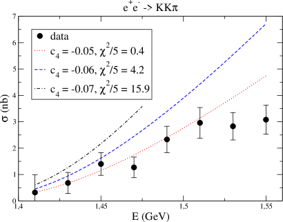
Figure 2: Comparison of the experimental data [28] with the theoretical prediction for the cross-section of the isovector component of $e^{+}e^{-}\rightarrow K^{*}(892)K\rightarrow K_{S}K^{\pm}\pi^{\mp}$ process, for different values of the $c_{4}$ coupling. The $\chi^{2}$ values are associated to the first 6 data points only.

Taking into account the input parameters quoted in Eq. (D) we obtain : $c_{4}\,=\,-0.047\pm 0.002$. The fit has been carried out for the first 6 bins (up to $E_{cm}\sim 1.52\,\mbox{GeV}$). This result corresponds to $\chi^{2}/dof=0.3$ and the displayed error comes only from the fit.

We take into consideration now the measured branching ratios for the $KK\pi$ channels of Table 1 in order to extract information both from $c_{4}$ and $g_{4}$. We notice that it is not possible to reconcile a prediction of the branching ratios of $\tau\rightarrow K\overline{K}\pi\nu_{\tau}$ and $\tau\rightarrow K^{-}K^{0}\pi^{0}\nu_{\tau}$ in spite of the noticeable size of the errors shown in the Table 1. Considering that the second process was measured long ago and that the $\tau^{-}\rightarrow K^{+}K^{-}\pi^{-}\nu_{\tau}$ decay has been focused by both CLEO III and BABAR we intend to fit the branching ratio of the latter. For the parameter values :

$$c_{4} = -0.07\pm 0.01\,,$$

$$g_{4} = -0.72\pm 0.20\,,$$ (50)

we find a good agreement with the measured widths $\Gamma(\tau^{-}\rightarrow K^{+}K^{-}\pi^{-}\nu_{\tau})$ and $\Gamma(\tau\rightarrow K^{-}K^{0}\pi^{0}\nu_{\tau})$ within errors (see Table 1). Notice that the value of $|c_{4}|$ is larger than that obtained from the fit to the $e^{+}e^{-}\rightarrow K_{S}K^{\pm}\pi^{\mp}$ data explained above. In Fig. 2 we show the first 8 bins in the isovector component of $e^{+}e^{-}\rightarrow K_{S}K^{\pm}\pi^{\mp}$ and the theoretical curves for different values of the $c_{4}$ coupling. As our preferred result we choose the larger value of $c_{4}$ in Eq. (4.1), since it provides a better agreement with the present measurement of $\Gamma(\tau^{-}\rightarrow K^{-}K^{0}\pi^{0}\nu_{\tau})$. Actually, one can expect a large incertitude in the splitting of isospin amplitudes in the $e^{+}e^{-}\rightarrow K_{S}K^{\pm}\pi^{\mp}$ cross-section (see Appendix C). Taking into account this systematic error, it could be likely that the theoretical curve with $c_{4}=-0.07$ falls within the error bars for the first data points.

5 Phenomenology of $\tau\rightarrow KK\pi\nu_{\tau}$ : Results and their analysis

Asymmetric B-factories span an ambitious $\tau$ programme that includes the determination of the hadron structure of semileptonic $\tau$ decays such as the $KK\pi$ channel. As commented in the Introduction the latest study of $\tau^{-}\rightarrow K^{+}K^{-}\pi^{-}\nu_{\tau}$ by the CLEO III Collaboration [7] showed a disagreement between the KS model, included in TAUOLA, and the data. Experiments with higher statistics such as BABAR and Belle should clarify the theoretical settings.

For the numerics in this Section we use the values in Appendix D. At present no spectra for these channels is available and the determinations of the widths are collected in Table 1.

Source	$\Gamma(\tau^{-}\to K^{+}K^{-}\pi^{-}\nu_{\tau})\,$	$\Gamma(\tau^{-}\to K^{0}\overline{K}^{0}\pi^{-}\nu_{\tau})\,$	$\Gamma(\tau^{-}\to K^{-}K^{0}\pi^{0}\nu_{\tau})\,$
PDG [35]	$3.103\,(136)$	$3.465\,(770)$	$3.262\,(521)$
BABAR [44]	$3.049\,(85)$
CLEO III [7]	$3.511\,(245)$
Belle [45]	$3.465\,(136)$
Our prediction	$3.4^{+0.5}_{-0.2}$	$3.4^{+0.5}_{-0.2}$	$2.5^{+0.3}_{-0.2}$

Table 1: Comparison of the measurements of partial widths (in units of $10^{-15}\,\mbox{GeV}$) with our predictions for the set of values in Eq. (4.1). For earlier references see [35].

We also notice that there is a discrepancy between the BABAR measurement of $\Gamma(\tau^{-}\rightarrow K^{+}K^{-}\pi^{-}\nu_{\tau})$ and the results by CLEO and Belle. Within $SU(2)$ isospin symmetry it is found that $\Gamma(\tau^{-}\rightarrow K^{+}K^{-}\pi^{-}\nu_{\tau})=\Gamma(\tau^{-}\rightarrow K^{0}\overline{K}^{0}\pi^{-}\nu_{\tau})$, which is well reflected by the values in Table 1 within errors. Moreover, as commented above, the PDG data [35] indicate that $\Gamma(\tau^{-}\rightarrow K^{-}K^{0}\pi^{0}\nu_{\tau})$ should be similar to $\Gamma(\tau^{-}\rightarrow K\overline{K}\pi\nu_{\tau})$. It would be important to obtain a more accurate determination of the $\tau^{-}\rightarrow K^{-}K^{0}\pi^{0}\nu_{\tau}$ width (the measurements quoted by the PDG are rather old) in the near future.

In our analyses we include the lightest resonances in both the vector and axial-vector channels, namely $\rho(775)$, $K^{*}(892)$ and $a_{1}(1260)$. It is clear that, as it happens in the $\tau\rightarrow\pi\pi\pi\nu_{\tau}$ channel (see Ref. [37]), a much lesser role, though noticeable, can be played by higher excitations on the vector channel. As experimentally only the branching ratios are available for the $KK\pi$ channel we think that the refinement of including higher mass resonances should be taken into account in a later stage, when the experimental situation improves.

In Figs. 3 and 4 we show our predictions for the normalized $M_{KK\pi}^{2}-$spectrum of the $\tau^{-}\rightarrow K^{+}K^{-}\pi^{-}\nu_{\tau}$ and $\tau^{-}\rightarrow K^{-}K^{0}\pi^{0}\nu_{\tau}$ decays, respectively. As discussed above we have taken $c_{4}=-0.07\pm 0.01$ and $g_{4}=-0.72\pm 0.20$ (notice that the second process does not depend on $g_{4}$). We conclude that the vector contribution ($\Gamma_{V}$) dominates over the axial-vector one ($\Gamma_{A}$) in both channels :

$$\frac{\Gamma_{A}}{\Gamma_{V}}\,\Big{|}_{K\overline{K}\pi}=\,0.16\pm 0.05\;,\;\;\;\;\frac{\Gamma_{A}}{\Gamma_{V}}\,\Big{|}_{K^{-}K^{0}\pi}=\,0.18\pm 0.04\;,\;\;\;\frac{\Gamma(\tau^{-}\rightarrow K^{+}K^{-}\pi^{-}\nu_{\tau})}{\Gamma(\tau^{-}\rightarrow K^{-}K^{0}\pi^{0}\nu_{\tau})}\,=\,1.4\pm 0.3\;,$$ (51)

where the errors estimate the slight variation due to the range in $c_{4}$ and $g_{4}$. These ratios translate into a ratio of the vector current to all contributions of $f_{v}=0.86\pm 0.04$ for the $K\overline{K}\pi$ channel and $f_{v}=0.85\pm 0.03$ for the $K^{-}K^{0}\pi$ one, to be compared with the result in Ref. [42], namely $f_{v}(K\overline{K}\pi)=0.20\pm 0.03$. Our results for the relative contributions of vector and axial-vector currents deviate strongly from most of the previous estimates, as one can see in Table 2. Only Ref. [5] pointed already to vector current dominance in these channels, although enforcing just the leading chiral constraints and using experimental data at higher energies.

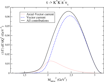
Figure 3: Normalized $M_{KK\pi}^{2}$-spectra for $\tau^{-}\rightarrow K^{+}K^{-}\pi^{-}\nu_{\tau}$. Notice the dominance of the axial-vector current at very low values of $Q^{2}$.

We conclude that for all $\tau\rightarrow KK\pi\nu_{\tau}$ channels the vector component dominates by far over the axial-vector one, though, as can be seen in the spectra in Figs. 3,4, the axial-vector current is the dominant one in the very-low $Q^{2}$ regime.

Source	$\Gamma_{V}/\Gamma_{A}$
Our result	$6\pm 2$
KS model [3]	$0.6-0.7$
KS model [46]	$0.4-0.6$
Breit-Wigner approach [5]	$\sim 9$
CVC [42]	$0.20\pm 0.03$
Data analysis [7]	$1.26\pm 0.35$

Table 2: Comparison of the ratio of vector and axial-vector contribution for $\tau\rightarrow KK\pi\nu_{\tau}$ partial widths. The last two lines correspond to the $\tau^{-}\rightarrow K^{+}K^{-}\pi^{-}\nu_{\tau}$ process only. Results in Ref. [46] are an update of Ref. [3]. The result of Ref. [42] is obtained by connecting the tau decay width with the CVC related $e^{+}e^{-}\rightarrow K_{S}K^{\pm}\pi^{\mp}$ (see Appendix C). The analysis in [7] was performed with a parameterization that spoiled the chiral normalization of the form factors.

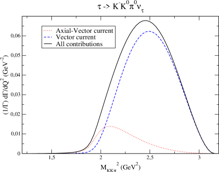
Figure 4: Normalized $M_{KK\pi}^{2}$-spectra for $\tau^{-}\rightarrow K^{-}K^{0}\pi^{0}\nu_{\tau}$. Notice the dominance of the axial-vector current at very low values of $Q^{2}$.

Next we contrast our spectrum for $\tau^{-}\rightarrow K^{+}K^{-}\pi^{-}\nu_{\tau}$ with that one arising from the KS model worked out in Refs. [3, 46]. This comparison is by no means straight because in these references a second and even a third multiplet of resonances are included in the analysis. As we consider that the spectrum is dominated by the first multiplet, in principle we could start by switching off heavier resonances. However we notice that, in the KS model, the $\rho(1450)$ resonance plays a crucial role in the vector contribution to the spectrum. This feature depends strongly on the value of the $\rho(1450)$ width, which has been changed from Ref. [3] to Ref. [46] . In Fig. 5 we compare our results for the vector and axial-vector contributions with those of the KS model as specified in Ref. [46] (here we have switched off the seemingly unimportant $K^{*}(1410)$). As it can be seen there are large differences in the structure of both approaches. Noticeably there is a large shift in the peak of the vector spectrum owing to the inclusion of the $\rho(1450)$ and $\rho(1700)$ states in the KS model together with its strong interference with the $\rho(770)$ resonance. In our scheme, including the lightest resonances only, the $\rho(1450)$ and $\rho(1700)$ information has to be encoded in the values of $c_{4}$ and $g_{4}$ couplings (that we have extracted in Subsection 4.1) and such an interference is not feasible. It will be a task for the experimental data to settle this issue.

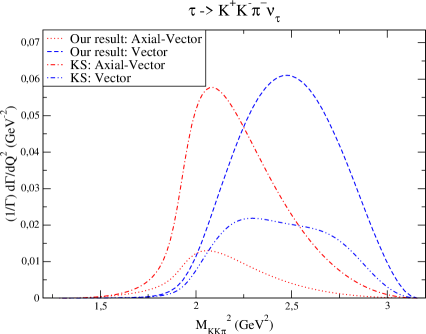
Figure 5: Comparison between the normalized $M_{KK\pi}^{2}$-spectra for the vector and axial-vector contributions to the $\tau^{-}\rightarrow K^{+}K^{-}\pi^{-}\nu_{\tau}$ channel in the KS model [46] and in our approach.

In Fig. 6 we compare the normalized full $M_{KK\pi}^{2}$ spectrum for the $\tau\rightarrow K\overline{K}\pi\nu_{\tau}$ channels in the KS model [46] and in our scheme. The most important feature is the large effect of the vector contribution in our case compared with the leading role of the axial-vector part in the KS model, as can be seen in Fig. 5. This is the main reason for the differences between the shapes of $M_{KK\pi}^{2}$ spectra observed in Fig. 6.

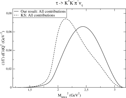
Figure 6: Comparison between the normalized $M_{KK\pi}^{2}$-spectra for $\tau^{-}\rightarrow K^{+}K^{-}\pi^{-}\nu_{\tau}$ in the KS model [46] and in our approach.

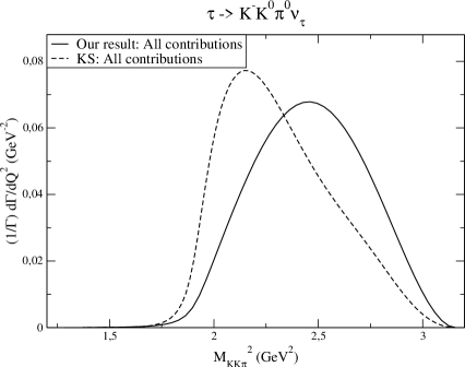
Figure 7: Comparison between the normalized $M_{KK\pi}^{2}$-spectra for $\tau^{-}\rightarrow K^{-}K^{0}\pi^{0}\nu_{\tau}$ in the KS model [46] and in our approach.

6 Conclusions

Hadron decays of the tau lepton are an all-important tool in the study of the hadronization process of QCD currents, in a setting where resonances play the leading role. In particular the final states of three mesons are the simplest ones where one can test the interplay between different resonance states. At present there are three parameterizations implemented in the TAUOLA library to describe the hadronization process in tau decays. Two are based on experimental data. The other alternative, namely the KS model, though successfull in the account of the $\pi\pi\pi$ final state, has proven to be unsuitable [7] when applied to the decays into $KK\pi$ hadron states. Our procedure, guided by large $N_{C}$, chiral symmetry and the asymptotic behaviour of the form factors driven by QCD, was already employed in the analysis of $\tau\rightarrow\pi\pi\pi\nu_{\tau}$ in Refs. [13] and [37], which only concern the axial-vector current. Here we have applied our methodology to the analysis of the $\tau\rightarrow KK\pi\nu_{\tau}$ channels where the vector current may also play a significant role.

We have constructed the relevant Lagrangian involving the lightest multiplets of vector and axial-vector resonances. Then we have proceeded to the evaluation of the vector and axial-vector currents in the large-$N_{C}$ limit of QCD, i.e. at tree level within our model. Though the widths of resonances are a next-to-leading effect in the $1/N_{C}$ counting, they have to be included into the scheme since the resonances do indeed resonate due to the high mass of the decaying tau lepton. We have been able to estimate the values of the relevant new parameters appearing in the Lagrangian with the exception of two, namely the couplings $c_{4}$ and $g_{4}$, which happen to be important in the description of $\tau\rightarrow KK\pi\nu_{\tau}$ decays. The range of values for these couplings has been determined from the measured widths $\Gamma(\tau^{-}\rightarrow K^{+}K^{-}\pi^{-}\nu_{\tau})$ and $\Gamma(\tau^{-}\rightarrow K^{-}K^{0}\pi^{0}\nu_{\tau})$.

In this way we provide a prediction for the —still unmeasured— spectra of both processes. We conclude that the vector current contribution dominates over the axial-vector current, in fair disagreement with the corresponding conclusions from the KS model [46] with which we have also compared our full spectra. On the other hand, our result is also at variance with the analysis in Ref. [42]. There are two all-important differences that come out from the comparison. First, while in the KS model the axial-vector contribution dominates the partial width and spectra, in our results the vector current is the one that rules both spectrum and width. Second, the KS model points out a strong interference between the $\rho(770)$, the $\rho(1450)$ and the $\rho(1700)$ resonances that modifies strongly the peak and shape of the $M_{KK\pi}$ distribution depending crucially on the included spectra. Not having a second multiplet of vector resonances in our approach, we cannot provide this feature. It seems strange to us the overwhelming role of the $\rho(1450)$ and $\rho(1700)$ states but it is up to the experimental measurements to settle this issue.

Even if our model provides a good deal of tools for the phenomenological analyses of observables in tau lepton decays, it may seem that our approach is not able to carry the large amount of input present in the KS model, as the later includes easily many multiplets of resonances. In fact, this is not the case, since the Lagrangian can be systematically extended to include whatever spectra of particles are needed. If such an extension is carried out the determination of couplings could be cumbersome or just not feasible, but, on the same footing as the KS model, our approach would provide a parameterization to be fitted by the experimental data. The present stage, however, has its advantages. By including only one multiplet of resonances we have a setting where the procedure of hadronization is controlled from the theory. This is very satisfactory if our intention is to use these processes to learn about QCD and not only to fit the data to parameters whose relation with the underlying theory is unclear when not directly missing.

We intend to follow our approach to analyse further relevant three pseudoscalar channels along the lines explained in this article.

Acknowledgements

 
 
      We wish to thank S. Eidelman, H. Hayashii, B. Malaescu, O. Shekhovtsova and Z. Was for their interest in this work and many useful discussions on the topic of this article. P. Roig has been partially supported by a FPU contract (MEC), the DFG cluster of excellence ’Origin and Structure of the Universe’ and a Marie Curie ESR Contract (FLAVIAnet). This work has been supported in part by the EU MRTN-CT-2006-035482 (FLAVIAnet), by MEC (Spain) under grant FPA2007-60323, by the Spanish Consolider-Ingenio 2010 Programme CPAN (CSD2007-00042) and by Generalitat Valenciana under grant PROMETEO/2008/069. This work has also been supported by CONICET and ANPCyT (Argentina), under grants PIP6009, PIP02495, PICT04-03-25374 and PICT07-03-00818.

Appendix A Definitions in the expressions of form factors

The results for the $F_{1}$, $F_{2}$ and $F_{3}$ form factors in $\tau\rightarrow KK\pi\nu_{\tau}$ decays given in Eqs. (3.1), (3.1), (3.1), (3.2), (3.2) and (3.2) are expressed in terms of the following functions :

$$A^{\mbox{\tiny R}}(Q^{2},x,y,m_{1}^{2},m_{2}^{2},m_{3}^{2}) = 3\,x\,+m_{1}^{2}-m_{3}^{2}+\left(1-\frac{2G_{V}}{F_{V}}\right)\left[2\,Q^{2}-2\,x-y+m_{3}^{2}-m_{2}^{2}\right]\,,$$

$$B^{\mbox{\tiny R}}(x,y,m_{1}^{2},m_{2}^{2}) = 2\,\left(m_{2}^{2}-m_{1}^{2}\right)\,+\,\left(1-\frac{2G_{V}}{F_{V}}\right)\left[y-x+m_{1}^{2}-m_{2}^{2}\right]\,,$$

$$A^{\mbox{\tiny RR}}(Q^{2},x,y,m_{1}^{2},m_{2}^{2},m_{3}^{2}) = \left(\lambda^{\prime}+\lambda^{\prime\prime}\right)\,(-3\,x+m_{3}^{2}-m_{1}^{2})\,$$

$$+\,\left(2\,Q^{2}+x-y+m_{1}^{2}-m_{2}^{2}\right)F\left(\frac{x}{Q^{2}}\,,\,\frac{m_{2}^{2}}{Q^{2}}\right)\,,$$

$$B^{\mbox{\tiny RR}}(Q^{2},x,y,z,m_{1}^{2},m_{2}^{2},m_{3}^{2}) = 2\left(\lambda^{\prime}+\lambda^{\prime\prime}\right)\left(m_{1}^{2}-m_{2}^{2}\right)+\left(y-x+m_{2}^{2}-m_{1}^{2}\right)F\left(\frac{z}{Q^{2}}\,,\,\frac{m_{3}^{2}}{Q^{2}}\right)\,,$$

$$C^{\mbox{\tiny R}}(Q^{2},x,m_{1}^{2},m_{2}^{2},m_{3}^{2}) = (c_{1}-c_{2}+c_{5})\,Q^{2}-(c_{1}-c_{2}-c_{5}+2c_{6})\,x$$

$$\,+(c_{1}+c_{2}+8c_{3}-c_{5})\,m_{3}^{2}+8\,c_{4}\,(m_{1}^{2}-m_{2}^{2})\,,$$

$$C^{\mbox{\tiny RR}}(Q^{2},x,m^{2}) = d_{3}\,(Q^{2}+x)+(d_{1}+8\,d_{2}-d_{3})\,m^{2}\,,$$

$$D^{\mbox{\tiny R}}(Q^{2},x,y) = (g_{1}+2\,g_{2}-g_{3})\,(x+y)-2\,g_{2}\,(Q^{2}+m_{K}^{2})$$

$$-(g_{1}-g_{3})\,(3\,m_{K}^{2}+m_{\pi}^{2})+2\,g_{4}\,(m_{K}^{2}+m_{\pi}^{2})+2\,g_{5}\,m_{K}^{2}\,,$$

$$E^{\mbox{\tiny R}}(x,y) = (g_{1}+2\,g_{2}-g_{3})\,(x-y)\,.$$ (A.1)

Here $u=Q^{2}-s-t+m_{1}^{2}+m_{2}^{2}+m_{3}^{2}$ and $F(x,y)=\lambda^{\prime\prime}+\lambda^{\prime}\,x-\lambda_{0}\,y$, where $\lambda_{0}$, $\lambda^{\prime}$ and $\lambda^{\prime\prime}$ are combinations of the $\lambda_{i}$ couplings defined in Eq. (15) :

$$-\sqrt{2}\,\lambda_{0} = 4\,\lambda_{1}+\lambda_{2}+\frac{\lambda_{4}}{2}+\lambda_{5}\,,$$

$$\sqrt{2}\,\lambda^{\prime} = \lambda_{2}-\lambda_{3}+\frac{\lambda_{4}}{2}+\lambda_{5}\,,$$ (A.2)

$$\sqrt{2}\,\lambda^{\prime\prime} = \lambda_{2}-\frac{\lambda_{4}}{2}-\lambda_{5}\,.$$

Appendix B $2\,g_{4}+g_{5}$ from $\omega\rightarrow\pi^{+}\pi^{-}\pi^{0}$

The process $\omega\rightarrow\pi^{+}(k_{1})\,\pi^{-}(k_{2})\,\pi^{0}(k_{3})$ provides us with an estimate for the combination of couplings $2\,g_{4}+g_{5}$. We will denote the polarization vector of the $\omega$ as $\varepsilon_{\omega}^{\sigma}$ and use the kinematic invariants $s_{ij}\,=\,(k_{i}\,+\,k_{j})^{2}$.

The amplitude for this process has two contributions. The first one, mediated by the $\rho(770)$ resonance was already studied in Ref. [24], where it was concluded that the contribution of a pure local amplitude was necessary to fulfill the phenomenological determinations. This piece can be obtained from our Lagrangian in Eq. (1/). The full result is given by :

$$i\,\mathcal{M}_{\omega\rightarrow\pi^{+}\pi^{-}\pi^{0}} = i\,\varepsilon_{\alpha\beta\rho\sigma}k_{1}^{\alpha}k_{2}^{\beta}k_{3}^{\rho}\varepsilon_{\omega}^{\sigma}\,\,\frac{8\,G_{V}}{M_{\omega}F^{3}}\,\times$$ (B.1)

$$\times\Bigg{\{}\frac{m_{\pi}^{2}(d_{1}\,+\,8\,d_{2}\,-\,d_{3})+(M_{\omega}^{2}\,+\,s_{12})d_{3}}{M_{\rho}^{2}\,-\,s_{12}}+\left\{s_{12}\to s_{13}\right\}+\left\{s_{12}\to s_{23}\right\}$$

$$\;\;\;\;\;\left.+\,\frac{\sqrt{2}}{G_{V}\,M_{V}}\left[(g_{1}\,-\,g_{2}\,-\,g_{3})(M_{\omega}^{2}\,-\,3\,m_{\pi}^{2})\,+\,3\,m_{\pi}^{2}(2\,g_{4}\,+\,g_{5})\right]\right\}\,,$$

where we have assumed ideal mixing between the states $|\,\omega_{8}\rangle$ and $|\,\omega_{1}\rangle$ :

$$|\,\omega\rangle\,=\,\sqrt{\frac{2}{3}}|\,\omega_{1}\rangle+\sqrt{\frac{1}{3}}|\,\omega_{8}\rangle\,.$$ (B.2)

Using the experimental figure for $\mbox{BR}(\omega\rightarrow\pi^{+}\pi^{-}\pi^{0})=0.892\pm 0.007$ [35], introducing the already known combinations of couplings as discussed in Sect. 4 and taking $G_{V}=F_{V}/F^{2}$ with $F_{V}$ given by Eq. (D) we find :

$$2\,g_{4}+g_{5}\,=\,-0.60\pm 0.02\,.$$ (B.3)

We will use this result to eliminate $g_{5}$ in terms of $g_{4}$, that remains unknown.

Appendix C Relation between $\sigma\left(e^{+}e^{-}\rightarrow KK\pi\right)$ and $\Gamma\left(\tau\rightarrow KK\pi\nu_{\tau}\right)$

Using $SU(2)_{I}$ symmetry, one can derive several relations between exclusive isovector hadron modes produced in $e^{+}e^{-}$ collisions and those related with the vector current ($F_{3}$ form factor) in $\tau$ decays. In particular we find :

$$\frac{\mathrm{d}}{\mathrm{d}Q^{2}}\,\Gamma\left(\tau^{-}\to K^{0}K^{-}\pi^{0}\nu_{\tau}\right)\Bigg{|}_{F_{3}}\,=\,f(Q^{2})\;\sigma_{I=1}\left(e^{+}e^{-}\to K^{-}K^{0}\pi^{+}\right)\,,$$ (C.1)

where

$$f(Q^{2})=\frac{G_{F}^{2}|V_{ud}|^{2}}{128(2\pi)^{5}M_{\tau}}\,\left(\frac{M_{\tau}^{2}}{Q^{2}}-1\right)^{2}\,\frac{1}{3}\,\left(1+\frac{2Q^{2}}{M_{\tau}^{2}}\right)\,\left(\frac{96\pi}{\alpha^{2}}\right)\,Q^{6}\,.$$ (C.2)

Analogously, one can also derive:

$$2\,\frac{\mathrm{d}}{\mathrm{d}Q^{2}}\,\Gamma\left(\tau\to K^{+}K^{-}\pi^{-}\nu_{\tau}\right)\Bigg{|}_{F_{3}} = f(Q^{2})\,\left[\sigma_{I=1}\left(e^{+}e^{-}\to K^{+}\overline{K}^{0}\pi^{-}\right)\,\right.$$

$$\;\;\;\;\;\;\;\;\;\;\;\;+\,2\,\sigma_{I=1}\left(e^{+}e^{-}\to K^{+}\,K^{-}\pi^{0}\right)\Big{]}\,.$$

Summing these equations one obtains :

$$\sum_{i=1}^{3}\frac{\mathrm{d}}{\mathrm{d}Q^{2}}\,\Gamma\left(\tau\to(KK\pi)_{i}\nu_{\tau}\right)\Bigg{|}_{F_{3}}\,=\,f(Q^{2})\,\sum_{i=1}^{4}\,\sigma_{I=1}\left(e^{+}e^{-}\to(KK\pi)_{i}\right)\,,$$ (C.4)

where the sums run over all possible charge channels in each case. If isovector and isoscalar components were splitted for all channels Eq. (C.4) would allow us to fit the data using our vector form factors for $\tau\to(KK\pi)_{i}\nu_{\tau}$.

BABAR has managed to split the isoscalar and isovector components in the cross sections $\sigma\left(e^{+}e^{-}\to K_{S}K^{\pm}\pi^{\mp}\right)$ [28]. The $I=1$ component of $\sigma\left(e^{+}e^{-}\to KK\,\pi\right)$ needs to be used, under the hypothesis of CVC, to obtain the spectral function of the processes $\tau\to KK\pi\nu_{\tau}$, and thus to help the extraction of $\alpha_{S}(M_{\tau})$ [42]. However, it is not straightforward to obtain the inclusive $I=1$ component of $\sigma\left(e^{+}e^{-}\to KK\pi\right)$ from the measured value of $\sigma\left(e^{+}e^{-}\to K_{S}^{0}K^{\pm}\pi^{\mp}\right)$. In fact, using only $SU(2)_{I}$ symmetry this is not possible. There are two further assumptions that need to be done in order to obtain the expression usually employed :

$$\sigma\left(e^{+}e^{-}\to KK\pi\right)\,=\,3\;\sigma\left(e^{+}e^{-}\to K_{S}K^{\pm}\pi^{\mp}\right)\,.$$ (C.5)

The first one is to assume that the processes $e^{+}e^{-}\to KK\pi$ are dominated by $K^{*}$-exchange. According to recent Dalitz plot analyses, [28] this is indeed a good approximation. However, $SU(2)_{I}$ symmetry and $K^{*}$ dominance do not allow to relate $\sigma\left(e^{+}e^{-}\to K_{S}K^{-}\pi^{+}\right)$ and $\sigma\left(e^{+}e^{-}\to K^{+}K^{-}\pi^{0}\right)$ as given by Eq. (C.5). Under $K^{*}$ dominance there are two intermediate chains that account for each final state :

$$A\left(K^{+}K^{-}\pi^{0}\right) = A\left(e^{+}e^{-}\to(K^{*-})\,K^{+}\to K^{-}\pi^{0}\,K^{+}\right)$$

$$+A\left(e^{+}e^{-}\to(K^{*+})\,K^{-}\to K^{+}\pi^{0}\,K^{-}\right)\;\equiv\,B\,+\,C\,,$$

$$A\left(K^{-}K^{0}\pi^{+}\right) = A\left(e^{+}e^{-}\to(K^{*+})\,K^{-}\to K^{0}\pi^{+}\,K^{-}\right)$$ (C.6)

$$+A\left(e^{+}e^{-}\to(\overline{K}^{*0})\,K^{0}\to\pi^{+}K^{-}\,K^{0}\right)\;\equiv\,\sqrt{2}\,\left(B\,-\,C\right)\,.$$

Accordingly we conclude that the relation $\sigma\left(e^{+}e^{-}\to K^{0}K^{-}\pi^{+}\right)=2\;\sigma\left(e^{+}e^{-}\to K^{+}K^{-}\pi^{0}\right)$, which is necessary to derive Eq. (C.5), can only be obtained by neglecting the interference terms arising from Eqs. (C).

We have checked the accuracy of this assumption using two different parameterizations for the involved hadronization amplitudes. First, we have employed a parameterization following the KS-like model used for tau decays into $KK\pi$ modes, using the values in Ref. [46]. Furthermore, we have used our expressions obtained within R$\chi$T in Sect. 3. In both cases, we have not set the contributions of other resonances than the $K^{*}$ to zero, although we have checked that they are of very little importance. With both kinds of parameterizations either at $\Gamma\left(\tau\to KK\pi\nu_{\tau}\right)$ or at $\sigma\left(e^{+}e^{-}\to KK\pi\right)$ the error of assuming that interference effects are negligible is at least of order 30 $\%$ in $e^{+}e^{-}$, being even larger in $\tau$ decays.

Parameterization	$\sigma\left(e^{+}e^{-}\to K^{0}K^{-}\pi^{+}\right)/2\,\sigma\left(e^{+}e^{-}\to K^{+}K^{-}\pi^{0}\right)$
[46]	$0.74$
R$\chi$T	$0.36$

Table C.1: Check of the validity of relation (C.5) -and thus of neglecting interference effects- for different hadronization parameterizations. The $Q^{2}$-endpoint in the cross-sections has been taken at $\sim 2$ GeV². We estimate the error of the R$\chi$T prediction to be around $30\,\%$.

In the same way, taking for granted the rightness of the very accurate assumptions of $SU(2)_{I}$ and $K^{*}$ dominance in $\tau\to KK\pi\nu_{\tau}$, it is still not possible to relate the widths to $K^{+}K^{-}\pi^{-}$ and $K^{-}K^{0}\pi^{0}$ in a model independent way. Under the hypothesis of negligible interference one would obtain

$$2\;\Gamma\left(\tau\to K^{+}K^{-}\pi^{-}\nu_{\tau}\right)=\Gamma\left(\tau\to K^{-}K^{0}\pi^{0}\nu_{\tau}\right)\,.$$ (C.7)

As can be observed in Table C.2, within the above considered models this relation does not hold.

Parameterization	$\Gamma\left(\tau\to K^{-}K^{0}\pi^{0}\right)/2\,\Gamma\left(\tau\to K^{+}K^{-}\pi^{-}\right)$
[46]	$0.62$
R$\chi$T	$0.36$

Table C.2: Check of the validity of relation (C.7) -and thus of neglecting interference effects- for different hadronization parameterizations. We estimate the error of the R$\chi$T prediction to be around $30\,\%$.

Appendix D Numerical input

For the numerics we use, if nothing is specified, the masses given in Ref. [35]. From the analyses of Refs. [37, 47] we use, as input, the following numerical values of the parameters that appear in our study :

$$F\,=\,0.0924\,\mbox{GeV}\; \;,\; \;F_{V}\,=\,0.180\,\mbox{GeV}\;\;\;\;\;\;\;,\;\;\;\;F_{A}\,=\,0.149\,\mbox{GeV}\;,$$

$$M_{V}\,=\,0.775\,\mbox{GeV}\; \;,\; \;M_{K^{*}}\,=\,0.8953\,\mbox{GeV}\;\;\;,\;\;\;\;M_{a_{1}}\,=\,1.120\,\mbox{GeV}\,.$$ (D.1)

Then we get $\lambda^{\prime}$, $\lambda^{\prime\prime}$ and $\lambda_{0}$ from the first equalities in Eq. (iii)). Incidentally we can also determine the value of $M_{A}\simeq 0.91\,\mbox{GeV}$. Notice that this value for $M_{A}$ is slightly lower than the result obtained in Ref. [26]. Our preferred set of values in Eq. (D) satisfies reasonably well all the short-distance constraints pointed out in Sect. 4, with a deviation from Weinberg sum rules of at most $10\%$, perfectly compatible with deviations due to the single resonance approximation.

References

• [1] A. Pich, Phys. Lett.  B 196 (1987) 561; A. Pich, Proceedings of the “Tau-charm factory workshop”, Ed. L.V. Beers, SLAC Rep.-343 (1989) 416; J. H. Kühn and A. Santamaría, Z. Phys.  C 48 (1990) 445.
• [2] R. Decker, E. Mirkes, R. Sauer and Z. Was, Z. Phys. C 58 (1993) 445; R. Decker and E. Mirkes, Phys. Rev. D 47 (1993) 4012; R. Decker, M. Finkemeier and E. Mirkes, Phys. Rev. D 50 (1994) 6863.
• [3] M. Finkemeier and E. Mirkes, Z. Phys.  C 69 (1996) 243 [arXiv:hep-ph/9503474].
• [4] C. Bruch, A. Khodjamirian and J. H. Kühn, Eur. Phys. J. C 39 (2005) 41 [arXiv:hep-ph/0409080].
• [5] J. J. Gómez-Cadenas, M. C. González-García and A. Pich, Phys. Rev. D 42 (1990) 3093.
• [6] G.J. Gounaris and J.J. Sakurai, Phys. Rev. Lett. 21 (1968) 244.
• [7] F. Liu [CLEO Collaboration], eConf C0209101 (2002) TU07 [Nucl. Phys. Proc. Suppl.  123 (2003) 66] [arXiv:hep-ex/0209025]; T. E. Coan et al. [CLEO Collaboration], Phys. Rev. Lett.  92 (2004) 232001 [arXiv:hep-ex/0401005].
• [8] J. Portolés, Nucl. Phys. Proc. Suppl.  144 (2005) 3 [arXiv:hep-ph/0411333]; P. Roig, AIP Conf. Proc.  964 (2007) 40 [arXiv:0709.3734 [hep-ph]].
• [9] R. Decker, S. Jadach, M. Jezabek, J.H. Kühn and Z. Was, Comput. Phys. Commun. 76 (1993) 361; ibid. 70 (1992) 69; ibid. 64 (1990) 275.
• [10] S. Weinberg, PhysicaA 96 (1979) 327; J. Gasser and H. Leutwyler, Annals Phys.  158 (1984) 142; J. Gasser and H. Leutwyler, Nucl. Phys. B 250 (1985) 465.
• [11] G. Colangelo, M. Finkemeier and R. Urech, Phys. Rev. D 54 (1996) 4403 [arXiv:hep-ph/9604279].
• [12] J. Portolés, Nucl. Phys. Proc. Suppl.  98 (2001) 210 [arXiv:hep-ph/0011303].
• [13] D. Gómez Dumm, A. Pich and J. Portolés, Phys. Rev. D 69 (2004) 073002 [arXiv:hep-ph/0312183].
• [14] G. ’t Hooft, Nucl. Phys. B 72 (1974) 461; G. ’t Hooft, Nucl. Phys. B 75 (1974) 461; E. Witten, Nucl. Phys. B 160 (1979) 57.
• [15] G. Ecker, J. Gasser, A. Pich and E. de Rafael, Nucl. Phys. B 321 (1989) 311.
• [16] J. F. Donoghue, C. Ramírez and G. Valencia, Phys. Rev. D 39 (1989) 1947.
• [17] S. Peris, M. Perrottet and E. de Rafael, JHEP 9805 (1998) 011 [arXiv:hep-ph/9805442];
M. Knecht, S. Peris, M. Perrottet and E. de Rafael, Phys. Rev. Lett.  83 (1999) 5230 [arXiv:hep-ph/9908283];
S. Peris, B. Phily and E. de Rafael, Phys. Rev. Lett.  86 (2001) 14 [arXiv:hep-ph/0007338].
• [18] A. Pich, in Phenomenology of Large-$N_{C}$ QCD edited by R.F. Lebed (World Scientific, Singapore, 2002), p. 239 [arXiv:hep-ph/0205030].
• [19] V. Cirigliano, G. Ecker, M. Eidemüller, R. Kaiser, A. Pich and J. Portolés, Nucl. Phys.  B 753 (2006) 139 [arXiv:hep-ph/0603205].
• [20] S.J. Brodsky and G.R. Farrar, Phys. Rev. Lett. 31 (1973) 1153; G.P. Lepage and S.J. Brodsky, Phys. Rev. D 22 (1980) 2157.
• [21] B. Moussallam, Nucl. Phys.  B 504 (1997) 381 [arXiv:hep-ph/9701400]; B. Moussallam, Phys. Rev.  D 51 (1995) 4939 [arXiv:hep-ph/9407402].
• [22] M. Knecht and A. Nyffeler, Eur. Phys. J. C 21 (2001) 659 [arXiv:hep-ph/0106034].
• [23] V. Cirigliano, G. Ecker, M. Eidemüller, A. Pich and J. Portolés, Phys. Lett. B 596 (2004) 96 [arXiv:hep-ph/0404004].
• [24] P. D. Ruiz-Femenía, A. Pich and J. Portolés, JHEP 0307 (2003) 003 [arXiv:hep-ph/0306157].
• [25] V. Cirigliano, G. Ecker, M. Eidemüller, R. Kaiser, A. Pich and J. Portolés, JHEP 0504 (2005) 006 [arXiv:hep-ph/0503108];
• [26] V. Mateu and J. Portolés, Eur. Phys. J.  C 52 (2007) 325 [arXiv:0706.1039 [hep-ph]].
• [27] G. Ecker, J. Gasser, H. Leutwyler, A. Pich and E. de Rafael, Phys. Lett. B 223 (1989) 425.
• [28] B. Aubert et al. [BaBar Collaboration], Phys. Rev.  D 77 (2008) 092002 [arXiv:0710.4451 [hep-ex]].
• [29] J. Wess and B. Zumino, Phys. Lett. B 37 (1971) 95; E. Witten, Nucl. Phys. B 223 (1983) 422.
• [30] G. Ecker, Prog. Part. Nucl. Phys.  35 (1995) 1 [arXiv:hep-ph/9501357]; A. Pich, Rept. Prog. Phys.  58 (1995) 563 [arXiv:hep-ph/9502366].
• [31] J. Bijnens, L. Girlanda and P. Talavera, Eur. Phys. J.  C 23 (2002) 539 [arXiv:hep-ph/0110400].
• [32] S. R. Coleman, J. Wess and B. Zumino, Phys. Rev.  177 (1969) 2239; C. G. Callan, S. R. Coleman, J. Wess and B. Zumino, Phys. Rev.  177 (1969) 2247.
• [33] M. Jamin, J. A. Oller and A. Pich, Nucl. Phys.  B 587 (2000) 331 [arXiv:hep-ph/0006045]; P. Buettiker, S. Descotes-Genon and B. Moussallam, Eur. Phys. J.  C 33 (2004) 409 [arXiv:hep-ph/0310283]; M. Jamin, J. A. Oller and A. Pich, Phys. Rev.  D 74 (2006) 074009 [arXiv:hep-ph/0605095]; S. Descotes-Genon and B. Moussallam, Eur. Phys. J.  C 48 (2006) 553 [arXiv:hep-ph/0607133].
• [34] B. Moussallam, Eur. Phys. J.  C 53 (2008) 401 [arXiv:0710.0548 [hep-ph]].
• [35] C. Amsler et al. [Particle Data Group], Phys. Lett.  B 667 (2008) 1.
• [36] J. H. Kühn and E. Mirkes, Z. Phys. C 56 (1992) 661 [Erratum-ibid. C 67 (1995) 364].
• [37] D. Gómez Dumm, P. Roig, A. Pich and J. Portolés, arXiv:0911.4436 [hep-ph].
• [38] D. Gómez Dumm, A. Pich and J. Portolés, Phys. Rev.  D 62 (2000) 054014 [arXiv:hep-ph/0003320].
• [39] H. Georgi, Nucl. Phys.  B 361 (1991) 339.
• [40] G. Amorós, S. Noguera and J. Portolés, Eur. Phys. J.  C 27 (2003) 243 [arXiv:hep-ph/0109169].
• [41] E. G. Floratos, S. Narison and E. de Rafael, Nucl. Phys. B 155 (1979) 115.
• [42] M. Davier, S. Descotes-Genon, A. Hocker, B. Malaescu and Z. Zhang, Eur. Phys. J.  C 56 (2008) 305 [arXiv:0803.0979 [hep-ph]].
• [43] S. Weinberg, Phys. Rev. Lett.  18 (1967) 507.
• [44] B. Aubert et al. [BABAR Collaboration], Phys. Rev. Lett.  100 (2008) 011801 [arXiv: 0707.2981 [hep-ex]].
• [45] I. Adachi et al. [Belle Collaboration], arXiv:0812.0480 [hep-ex].
• [46] M. Finkemeier, J. H. Kühn and E. Mirkes, Nucl. Phys. Proc. Suppl.  55C (1997) 169 [arXiv:hep-ph/9612255].
• [47] M. Jamin, A. Pich and J. Portolés, Phys. Lett.  B 664 (2008) 78 [arXiv:0803.1786 [hep-ph]].
• [48] R. Barate et al. [ALEPH Collaboration], Eur. Phys. J.  C 4 (1998) 409.