Near–IR integral field spectroscopy of ionizing stars and young stellar objects on the borders of H ii regions

Abstract

Aims. We study three Galactic H ii regions – RCW 79, RCW 82 and RCW 120 – where triggered star formation is taking place. Two stellar population are observed: the ionizing stars of each H ii region and young stellar objects on their borders. Our goal is to show that they represent two distinct populations, as expected from successive star forming events.

Methods. We use near–infrared integral field spectroscopy obtained with SINFONI on the VLT to make a spectral classification. We derive the stellar and wind properties of the ionizing stars using atmosphere models computed with the code CMFGEN. The young stellar objects are classified according to their $K$–band spectra. In combination with published near and mid infrared photometry, we constrain their nature. Linemaps are constructed to study the geometry of their close environment.

Results. We identify the ionizing stars of each region. RCW 79 is dominated by a cluster of a dozen O stars, identified for the first time by our observations. RCW 82 and RCW 120 are ionized by two and one O star, respectively. All ionizing stars are early to late O stars, close to the main sequence. The cluster ionizing RCW 79 formed 2.3$\pm$0.5 Myr ago. Similar ages are estimated, albeit with a larger uncertainty, for the ionizing stars of the other two regions. The total mass loss rate and ionizing flux is derived for each regions. In RCW 79, where the richest cluster of ionizing stars is found, the mechanical wind luminosity represents only 0.1% of the ionizing luminosity, questioning the influence of stellar winds on the dynamics of these three H ii regions. The young stellar objects show four main types of spectral features: H₂ emission, Br$\gamma$ emission, CO bandheads emission and CO bandheads absorption. These features are typical of young stellar objects surrounded by disks and/or envelopes, confirming that star formation is taking place on the borders of the three H ii regions. The radial velocities of most YSOs are consistent with that of the ionized gas, firmly establishing that their association with the H ii regions. Exceptions are found in RCW 120 where differences up to 50 km s^-1 are observed. Outflows are detected in a few YSOs. All YSOs have moderate to strong near–IR excess. In the [24] versus $K-$[24] diagram, the majority of the sources dominated by H₂ emission lines stand out as redder and brighter than the rest of the YSOs. The quantitative analysis of their spectra indicates that for most of them the H₂ emission is essentially thermal and likely produced by shocks. We tentatively propose that they represent an earlier phase of evolution compared to sources dominated by Br$\gamma$ and CO bandheads. We suggest that they still possess a dense envelope in which jets or winds create shocks. The other YSOs have partly lost their envelopes and show signatures of accretion disks. Overall, the YSOs show distinct spectroscopic signatures compared to the ionizing sources, confirming the presence of two stellar populations.

1 Introduction

Massive stars play a significant role in several fields of astrophysics. They produce the majority of heavy elements and spread them in the interstellar medium, taking an active part in the chemical evolution of galaxies. But they also end their life as supernovae and gamma–ray bursts. Through their strong winds and ionizing fluxes they power H ii regions and bubbles which are often used to trace metallicity gradients in galaxies. The energy they release in the interstellar medium is thought to trigger second–generation star formation events. Observations of young stellar objects (YSO) in molecular clouds surrounding (clusters of) massive stars lend support to this mechanism (e.g. Walborn et al. 2002; Hatano et al. 2006).

A particular case concerns star formation on the borders of H ii regions. According to the collect and collapse model (Elmegreen & Lada 1977), a dense shell of material is trapped between the shock and ionization front of an expanding H ii regions. When the amount of collected material is large enough, global shell fragmentation occurs and new stars are formed. The observation of molecular condensations on the borders of several H ii regions and the subsequent identification of YSOs within these clumps (Deharveng et al. 2003, 2005; Zavagno et al. 2006, 2007; Deharveng et al. 2008, 2009; Pomarès et al. 2009) confirms that this mechanism is at work at least in some H ii regions.

Other mechanisms leading to triggered star formation exist. Some work qualitatively as the collect and collapse model in the sense that the clumps are formed during the H ii region expansion. For instance, dynamical instabilities of the ionization front (Vishniac 1983; Garcia-Segura & Franco 1996) create molecular condensations separated by zones of lower densities. The newly formed clumps grow until they become Jeans unstable and collapse. Alternatively, second generation star formation can happen in pre-existing clumps. If the neutral gas in which the H ii region expands is not homogeneous, the outer layers of the molecular overdensities are ionized like the borders of a classical H ii region. A shock front precedes the ionization front inside these clumps, leading to their collapse (Duvert et al. 1990; Lefloch & Lazareff 1994).

A number of questions regarding triggered star formation remain unanswered. The properties of the observed YSOs are poorly known besides a crude classification in class I or class II objects by analogy with low–mass stars. YSOs usually display near–infrared spectra with CO, Br$\gamma$ and/or H₂ emission lines (Bik et al. 2006). The relation, if any, between objects with different spectroscopic appearance is not clear. Besides, in the regions where the collect and collapse process is at work, the quantitative properties of the ionizing sources of the H ii regions are not known. In particular, the relative role of ionizing radiation and stellar winds on the dynamics of such regions is debated. The timescales under which material accumulates and fragments, and the properties of the resulting clumps depend on the strength of those two factors (Whitworth et al. 1994). Hence, one might wonder whether the nature of the newly formed objects depends on the properties of the stars powering the H ii regions.

In the present study, we tackle these questions by investigating the properties of the ionizing stars and YSOs of three Galactic H ii regions: RCW 79, RCW 82 and RCW 120 (Rodgers et al. 1960). Those regions are known to be the sites of triggered star formation (Zavagno et al. 2006, 2007; Pomarès et al. 2009; Kang et al. 2009). We have used SINFONI on the VLT to obtain near–infrared spectra of both the ionizing stars and a selection of YSOs in each region. Our main goals were:

• Identify the ionizing stars of each region, and derive their stellar properties using atmosphere models. In particular, we want to determine their ionizing fluxes and mass loss rates in order to better understand the dynamics of the H ii regions. Equally important is the determination of the age of those stars, since it can be related to the presence of YSOs to quantitatively confirm the existence of triggered star formation.

• Constrain the nature of the YSOs on the borders of the H ii regions. In combination with infrared photometry, spectroscopy can reveal the presence of disks or envelopes. The evolutionary status of those objects can thus be better understood. In particular, it can be clearly shown whether they are stars still in their formation process or objects already on the main sequence.

The paper is organized as follows. In Sect. 2 we present the three H ii regions targeted in this study. Sect. 3 describes our observations. The analysis of the ionizing stars is presented in Sect. 4, while the YSOs are discussed in Sect. 5. We discuss our results in Sect. 6 and summarize our conclusions in Sect. 7.

2 Presentation of the observed H ii regions

2.1 RCW 79

RCW 79 is a Southern Galactic H ii region located at 4.2$\pm$1 kpc (Russeil et al. 1998). Its diameter is $\sim$6.4 pc. Zavagno et al. (2006) (hereafter ZA06) used Spitzer GLIMPSE and SEST-SIMBA 1.2-mm continuum data to study the star formation on the borders of this region. A layer of warm dust is clearly seen at 8 $\mu$m surrounding RCW 79 (Fig. 1). A compact H ii region is observed in this layer as well as five cold dust condensations (masses between 100 and 1000 M_⊙) detected by 1.2-mm continuum emission. YSOs have also been revealed by Spitzer-GLIMPSE observations, leading ZA06 to conclude that triggered massive star formation was at work possibly through the collect and collapse process (Elmegreen & Lada 1977). Eight YSOs detected in the near IR have been observed with SINFONI at the VLT. They are identified on Fig. 1. In several cases, multiple sources have been uncovered by the SINFONI observations reported in this paper. They are identified in Sect. 5 and Appendix B.

The ionizing stars of RCW 79 were unknown before the present study. Using photometry and choosing objects inside the H ii region contours, we have identified and observed a cluster of possible OB stars candidates (blue square in Fig. 1). They are described in Sect. 4.

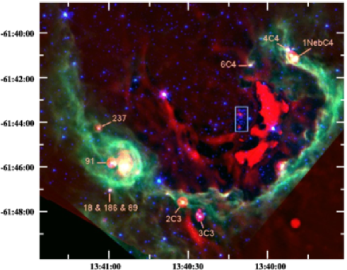
Figure 1: Identification of the RCW 79 YSOs targeted in the present study on a composite infrared color image. Blue and green are the Siptzer–GLIMPSE images at 3.6 and 8.0 $\mu$m respectively. Red is an unsharped masked image obtained from the Spitzer–MIPS frame at 24 $\mu$m (as explained in ZA07). The bright extended emission has been subtracted to emphasize the YSOs. The candidate ionizing sources are located inside the blue rectangle (see also Fig. 4).

2.2 RCW 82

RCW 82 is a Southern H ii region located at a distance of 3.4$\pm$1 kpc. Its radius is about 5 pc. Pomarès et al. (2009) (hereafter PO09) detected molecular material in ¹²CO(1-0) and ¹³CO(1-0) surrounding the H ii region. They showed that some of the structures correspond to dense material collected between the shock front and the ionization front during the expansion of the H ii region. Masses of these clumps range from 200 to 2500 M_⊙. Star formation is observed on the borders of RCW 82, with a total of 63 candidate YSOs. Among these, we have selected five YSO candidates visible in the $K$–band for our study. These objects are shown on Fig. 2.

PO09 identified four candidate ionizing sources, among which two are likely O stars (see their Fig. 5). These sources are located just south of the 24 $\mu$m emission ridge in Fig 2, and better displayed in the upper panel of Fig. 5.

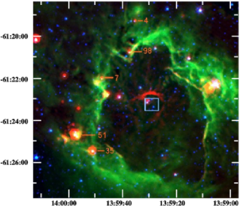
Figure 2: Same as Fig. 1 for RCW 82.

2.3 RCW 120

A detailed study of RCW 120 can be found in Zavagno et al. (2007) (hereafter ZA07), Deharveng & Zavagno (2008) (DE08) and Deharveng et al. (2009) (DE09). RCW 120 is the nearest of the three H ii regions observed in the present study. Its distance, D=1.35$\pm$0.3 kpc, is well determined since both the photometric and kinematic distances are in good agreement (DE09).

RCW 120 has a circular geometry (diameter $\sim$3.5 pc) and is surrounded by a shell of dense material collected during the expansion of the H ii region. The cold dust emission of this shell has been observed with the ESO SEST at 1.2-mm (ZA07) and with the APEX-LABOCA camera at 870 $\mu$m (DE09). Its mass is in the range 1100–1900 M_⊙; it is fragmented with massive fragments elongated along the ionization front. Star formation is at work in these condensations, as discussed by ZA07 and DE09. Twelve candidate YSOs have been observed with SINFONI and are identified in Fig. 3.

The central ionizing star of RCW 120 is CD$-$38^∘11636. Its spectral type (estimated from spectrograms) is O8 (Georgelin & Georgelin 1970) or O9 (Crampton 1971) - see also the discussion in DE08. Its extinction, determined by Avedisova & Kondratenko (1984) is A_V=4.65 mag. It is located just north of the bright 24 $\mu$m emission ridge in Fig. 3. Its characteristics are discussed in Sect. 4.

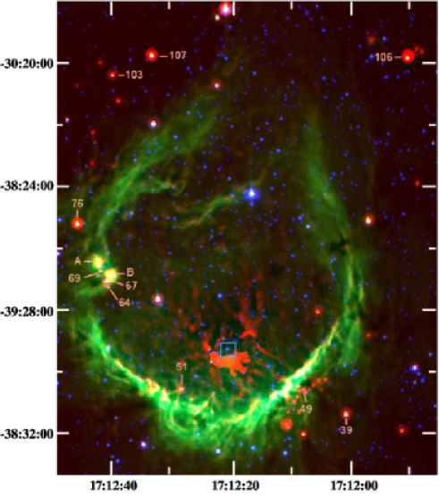
Figure 3: Same as Fig. 1 for RCW 120. On this image, the extended high brightness emission has been subtracted to enhance the small scale structures and the point sources.

3 Observations and data reduction

For the current project, we selected two types of sources: the candidate ionizing stars of the H ii regions and a few candidate YSOs. For the latter, we selected the brightest objects in the $K$–band.

Data have been collected at the ESO-VLT on April 25^th and 26^th 2008. The near infrared integral field spectrograph SINFONI (Eisenhauer et al. 2003) was used in seeing–limited mode to obtain medium resolution $K$–band spectra of our selected sources. We selected the 250 mas scale which provided a field of view of 8″$\times$8″. Sequences of source and sky exposures were conducted in order to ensure optimal sky subtraction. For the faintest sources, two exposures were made, with a 1″ offset between them to minimize pixels artifacts. The exposure times ranged from 1 minute for $K$=9 sources to 10 minutes for $K$=13 objects. Telluric stars were observed regularly during the night to allow proper atmospheric correction. Standard calibration data were obtained by the ESO staff. The observations were conducted under an optical seeing ranging from 0.6″ to 1.2″.

Data reduction was made with the SPRED software (Abuter et al. 2006). After bias subtraction, flat field and bad pixel corrections, wavelength calibration was done using a Ne-Ar spectrum. Fine tuning was subsequently performed using sky lines. Telluric correction was done using standard stars from which Br$\gamma$ and, when present, He i 2.112 $\mu$m were removed. The resulting spectra have a signal to noise of 10-100 depending on the source brightness and wavelength. Their resolution is $\sim$ 4000 (see also Sect. 5.4). They were extracted with the software QFitsView , carefully selecting individual “source” pixels one by one to avoid contamination by neighboring objects. Background pixels were selected close to the “source” pixels in order to correct for the underlying nebular emission. In practice, the average spectrum of these background pixels is subtracted to the each individual source pixels. Then all corrected source pixels are added together to ensure optimum extraction of the pure stellar sprectrum. This method is possible with integral field spectroscopy and was one of the main drivers for the choice of SINFONI for the present observations.

4 Ionizing stars

In this section we describe the spectral morphology of the ionizing sources of each region. We determine their stellar and wind properties using atmosphere models computed with the code CMFGEN (Hillier & Miller 1998). Fig. 4 shows the cluster of stars responsible for the ionization of RCW 79. The stars are labeled on the 2MASS $K$–band image presented on the left part of the figure. Numbers correspond to decreasing 2MASS $K$–band magnitudes. Note that star number 3 is not indicated: it corresponds to a source out of the field which turned out to be a foreground star (its spectrum displays CO bandheads in absorption typical of cool, evolved stars). The right panel of Fig. 4 shows a mosaic of the SINFONI fields observed. In many cases, the higher spatial resolution reveals several components for the same 2MASS source (e.g. source 9). Consequently, we have assigned new names to the resolved components. The identification is shown on the right side of Fig. 4. Similarly, the ionizing sources of RCW 82 and RCW 120 are displayed in Fig. 5.

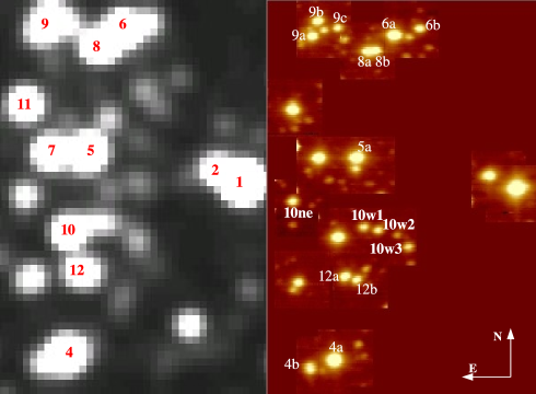
Figure 4: $K$–band images of the ionizing star cluster of RCW79 from 2MASS (left) and SINFONI (right). The intensity of the SINFONI image corresponds to the median of the spectral dimension of the datacube.

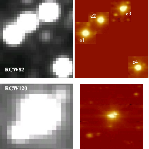
Figure 5: Same as Fig. 4 for RCW 82 (top) and RCW 120 (bottom). North is up and East is left.

4.1 Photometry and spectral classification

Table 1 summarizes the observational properties of the ionizing stars of the three regions. Photometry is from 2MASS. When a given 2MASS point source was resolved in several components by our observations, the relative SINFONI fluxes were used to recompute the individual magnitudes, using the 2MASS magnitude as a measure of the total flux from all components. In addition, the $K$–band magnitude of star 2 was revised because its magnitude is clearly different from that of star 1, in contradiction to the the 2MASS values (see right panel of Fig. 4). Inspection of the 2MASS catalog revealed that the aperture used to compute the $K$–band magnitude was wider than the separation of sources 1 and 2. Hence, the flux used to estimate the $K$–band magnitude of star 2 was contaminated by flux from star 1. We used the SINFONI flux and 2MASS magnitude of star 1 to calibrate the $K$–band magnitude of star 2 from the observed SINFONI flux. The $H$–band magnitudes are from 2MASS. Since there is no SINFONI $H$–band data, one cannot recalculate the magnitude of the components of unresolved 2MASS sources. In that case, we give the 2MASS $H$–band magnitude as a lower limit.

For each region, we calculated the absolute $K$–band magnitude using information on the distance and extinction:

• RCW 79: a distance of 4.2$\pm$1 kpc was derived by Russeil et al. (1998). We estimated the $K$–band extinction from the $H-K$ color of the early type stars of the region (see below for the spectral classification). Since ($H-K$)₀ is basically independent of the spectral type for O stars (see Martins & Plez 2006), one can use the 2MASS magnitudes even in the cases were SINFONI revealed several sub-components. In practice, we used stars 4, 5, 7, 8, 9 and 10 to obtain A_K = 0.7 $\pm$ 0.1.

• RCW 82: We proceeded as for RCW 79 to calculate MK assuming a distance of 3.4$\pm$1 kpc (Russeil et al. 1998). The extinction estimate was based on stars RCW82 e2 and RCW82 e3. Both of them are O stars. A mean value of A_K=0.36$\pm$0.2 was derived.

• RCW 120: With a distance of 1.35$\pm$0.3 kpc (ZA07), RCW 120 is the closest region of our sample. The region is ionized by a single O star. The estimated extinction is A_K=0.50 $\pm$ 0.1. This is in good agreement with previous estimates (see Sect. 2.3).

Figs 18 and 19 show the spectra of the candidate ionizing stars of RCW 79, RCW 82 and RCW 120. Most of the stars show Br$\gamma$ and He i 2.112 $\mu$m absorption and, depending on the sources, He ii 2.189 $\mu$m absorption, C iv 2.070–2.083 $\mu$m emission and the N iii/C iii/O iii emission complex at 2.115 $\mu$m. These features are typical of OB stars. We relied on the atlases of $K$–band spectra of Hanson et al. (1996, 2005) to assign spectral types to the ionizing stars of RCW 79, RCW 82 and RCW 120. In practice, we have used the following scheme:

• the presence of He ii 2.189 $\mu$m indicates a spectral type earlier than O8

• C iv 2.070–2.083 $\mu$m emission is observed in O4-6 stars and is the strongest at O5

• the N iii–C iii–O iii emission complex is observed in emission together with He i 2.112 $\mu$m in absorption in O4-O7 stars

• He i 2.112 $\mu$m disappears at spectral types later than B2.5

• O3–7 supergiants have Br$\gamma$ either in emission or in absorption weaker than He ii 2.189 $\mu$m. Later type supergiants have a narrow Br$\gamma$ absorption profile from which He i 2.164 $\mu$m is clearly separated. Dwarfs and giants have broader Br$\gamma$ absorption (He i 2.164 $\mu$m is blended with Br$\gamma$).

Based on these features, we classified the ionizing stars as OB dwarfs or giants. The results are listed in Table 1. The earliest spectral types are O4–6 and are observed only in the richest ionizing cluster (RCW 79). Most stars are late O – early B dwarfs/giants. We do not observe any supergiant. The distinction between dwarfs and giants is not easily feasible with our spectra. Hence we adopt the conservative approach to give the luminosity class V/III to most of our stars. Some of the stars did not show any of the above features. Instead, strong CO bandheads were clearly visible. Such spectra are typical of cool, evolved low mass stars . They do not contribute any ionizing flux and are most likely foreground or background stars. We classify them as “late” in Table 1. Three stars also show strong He i 2.056 $\mu$m and Br$\gamma$ emission, without He i 2.112 $\mu$m emission. In one case (RCW82 e1), the H i Pfund serie and Mg ii 2.138–2.144 $\mu$m were also detected in emission. According to Hanson et al. (1996) (see also Clark & Steele 2000), these features are seen in Oe–Be stars. Such objects are thought to host a circumstellar disk contributing a significant fraction of the near-IR emission (both line and continuum). Note that the ionizing source of RCW 120 seems to be double (Fig. 5). We tried to extract the spectra of both components, but found no difference between them. This indicates either that both components have the same spectral type, or that the spatial resolution of our observations is not sufficient to separate the spectra. Hence, we have treated the ionizing source of RCW 120 as a single source.

PO09 estimated a spectral type 06.5V and 07.5V for stars RCW82 e2 and RCW82 e3 respectively from $J$ vs $J-K$ and $J-H$ vs $H-K$ diagrams. Our spectroscopic classification indicates later types: O9-B2V/III for both stars. Given the difficulty to make a spectral classification from near-infrared color–color and color–magnitude diagrams, the difference is acceptable. Similarly, star RCW82 e4 is identified as a late–type giant which is confirmed by our spectroscopy. PO09 showed that star RCW82 e1 presented a near-IR excess, which is consistent with the presence of a disk in a star of spectral type Oe or Be. ZA07 reported a spectral type O8V for the ionizing star of RCW 120. We prefer a spectral type O6–8V/III, in rather good agreement. Finally, the ionizing sources of RCW 79 were not previously identified. ZA06 estimated that a single O4V star could power the H ii region. This is roughly consistent with our finding that a cluster of about ten O4 to O9 stars is responsible for the ionization.

Table 1: Position and photometry of ionizing stars.

Source	RA	DEC	$H$	$K$	MK	ST
	h m s	${}^{\circ}\arcmin\ \arcsec$
RCW79 1	13:40:09.11	-61:43:51.9	9.10$\pm$0.04	8.29$\pm$0.03	-5.53$\pm$0.53	OBe
RCW79 2	13:40:09.64	-61:43:50.1	$>$10.59	10.41$\pm$0.06	-3.46$\pm$0.53	O7.5–8V/III
RCW79 4a	13:40:12.63	-61:44:16.0	$>$9.41	9.23$\pm$0.02	-4.64$\pm$0.53	O4–6V/III
RCW79 4b	13:40:13.10	-61:44:17.1	$>$9.41	11.29$\pm$0.02	-2.54$\pm$0.53	?
RCW79 5a	13:40:12.19	-61:43:47.6	$>$9.40	9.24$\pm$0.05	-4.62$\pm$0.53	O4–6V/III
RCW79 6a	13:40:11.47	-61:43:30.6	$>$9.24	9.65$\pm$0.07	-4.22$\pm$0.53	O6–8V/III
RCW79 6b	13:40:10.98	-61:43:29.6	$>$9.24	11.65$\pm$0.07	-2.22$\pm$0.53	O9–B2V
RCW79 6c	13:40:11.17	-61:43:30.9	$>$9.24	12.97$\pm$0.07	-0.86$\pm$0.53	$>$B2.5V
RCW79 7	13:40:12.93	-61:43:47.8	9.93$\pm$0.04	9.64$\pm$0.03	-4.23$\pm$0.53	O6–8V/III
RCW79 8a	13:40:11.98	-61:43:32.9	$>$9.93	10.33$\pm$0.04	-3.54$\pm$0.53	O9–B2V/III
RCW79 8b	13:40:11.82	-61:43:32.7	$>$9.93	10.55$\pm$0.04	-3.32$\pm$0.53	O9–B2V/III
RCW79 9a	13:40:13.06	-61:43:30.6	$>$10.12	10.79$\pm$0.03	-3.07$\pm$0.53	O9–B2V/III
RCW79 9b	13:40:12.95	-61:43:28.6	$>$10.12	10.91$\pm$0.03	-2.96$\pm$0.53	O9–B2V/III
RCW79 9c	13:40:12.56	-61:43:29.5	$>$10.12	11.87$\pm$0.03	-1.95$\pm$0.53	B
RCW79 10	13:40:12.56	-61:43:58.9	10.09$\pm$0.07	9.84$\pm$0.05	-4.05$\pm$0.53	O6.5–8V/III
RCW79 10ne	13:40:13.44	-61:43:53.9	12.71$\pm$0.09	11.25$\pm$0.03	-2.57$\pm$0.53	Be
RCW79 10w1	13:40:12.06	-61:43:57.4	$>$11.69	12.11$\pm$0.05	-1.71$\pm$0.53	B0-2.5V
RCW79 10w2	13:40:11.79	-61:43:57.8	$>$11.69	12.04$\pm$0.05	-1.78$\pm$0.53	B0-2.5V
RCW79 10w3	13:40:11.19	-61:44:00.1	12.31$\pm$0.10	11.99$\pm$0.07	-1.83$\pm$0.53	B1-2
RCW79 11	13:40:13.44	-61:43:41.0	10.39$\pm$0.04	9.93$\pm$0.03	–	late
RCW79 12a	13:40:12.42	-61:44:04.2	$>$10.67	10.75$\pm$0.04	–	late
RCW79 12b	13:40:12.19	-61:44:04.9	$>$10.67	11.49$\pm$0.04	-2.38$\pm$0.53	O9–B2V/III
RCW79 CHII 6	13:40:53.71	-61:45:46.8	11.55$\pm$0.07	10.72$\pm$0.05	-4.03$\pm$0.53	O7.5–9.5V/III
RCW82 e1	13:59:29.86	-61:23:08.9	9.55$\pm$0.03	9.09$\pm$0.02	–	Be
RCW82 e2	13:59:29.13	-61:23:04.2	9.59$\pm$0.08	9.40$\pm$0.03	-3.62$\pm$0.67	O9–B2V/III
RCW82 e3	13:59:28.09	-61:23:00.4	9.41$\pm$0.03	9.19$\pm$0.03	-3.83$\pm$0.67	O9–B2V/III
RCW82 e4	13:59:27.37	-61:23:20.3	10.44$\pm$0.02	9.35$\pm$0.02	–	late
RCW120 e	17:12:20.82	-38:29:25.5	7.71$\pm$0.04	7.52$\pm$0.02	-3.62$\pm$0.49	O6–8V/III

4.2 Spectroscopic analysis

In this section we derive the stellar and wind properties of the ionizing stars of the H ii regions by means of spectroscopic analysis with atmosphere models. We subsequently use the derived properties to constrain the age of the ionizing populations.

4.2.1 Stellar and wind properties

The stellar and wind properties have been derived through spectroscopic analysis. Atmosphere models were computed with the code CMFGEN (Hillier & Miller 1998). This code solves the radiative transfer and statistical equations in the co-moving frame of the expanding atmosphere, for light elements as well as for metals. It thus produces non-LTE, line blanketed atmosphere models with winds. An exhaustive description of the code and its approximations is given in Hillier & Miller (1998). Summaries of the main characteristics can also be found in Hillier et al. (2003); Martins et al. (2008). The resulting synthetic spectra are compared to the SINFONI $K$–band spectra to constrain the main physical parameters. In practice, we have proceeded as follows:

• Effective temperature: the determination of T_eff usually relies on the ratio of He i to He ii lines. We have used the following lines: He i 2.112 $\mu$m and He ii 2.189 $\mu$m when present. C iv 2.07–2.08 $\mu$m lines are used as secondary indicators since they appear in emission in the hottest O stars (Hanson et al. 1996). An uncertainty of 2000 to 3000K is achieved depending on the star. For stars cooler than $\sim$32000 K He ii 2.189 $\mu$m vanishes. The uncertainty on T_eff is large (5000 K) and is set by the presence and strength of He i lines.

• Mass loss rate: The main indicator in the $K$–band spectrum of O stars is Br$\gamma$. It is filled by emission as the wind strength increases. We have used this line to constrain the mass loss rates of the ionizing stars. However, as demonstrated below, it becomes almost insensitive to $\dot{M}$ below $\sim 3\times 10^{-8}M_{\odot}yr^{-1}$ so that we could derive only upper limits on $\dot{M}$. We stress once more that our correction for nebular contamination ensures the best extraction possible of the stellar line profiles. Thus, our mass loss rate determination does not suffer from major uncertainties due to non stellar emission.

• Luminosity: $\log\frac{L}{L_{\odot}}$ was derived from the absolute magnitude and the $K$–band bolometric correction. The latter was computed from T_eff and the calibration of Martins & Plez (2006). The uncertainty on $\log\frac{L}{L_{\odot}}$ was calculated from a full error propagation and takes into account the uncertainties on the distance, T_eff and A_K. It is of the order 0.2 dex for stars in the three regions.

Several parameters could not be derived due to the lack of spectral diagnostics. In particular, the surface gravity was adopted. Since most of our stars are dwarfs/giants, we chose $\log g=4.0$ which is typical of O dwarfs (Martins et al. 2005a). In principle Br$\gamma$ can be used to constrain $\log g$ (e.g. Repolust et al. 2005). However, the S/N of a few tens combined to the medium resolution of our spectra prevents an accurate determination. Besides, since we use this line to determine mass loss rates and since the line core depends not only on $\dot{M}$ but also on $\log g$ (although in a less sensitive way), we decided to fix $\log g$.

Modern atmosphere models for massive stars also include clumping since evidence for wind inhomogeneities exist (e.g. Hillier 1991; Hillier et al. 2003; Lépine & Moffat 1999). Clumping is usually quantified by a volume filling factor $f$. Currently, no diagnostics of clumping have been identified in the K–band spectra of O stars with moderate winds. Such diagnostics are traditionally found in the UV, optical and submm range (Hillier 1991; Eversberg et al. 1998; Blomme et al. 2002). Hence, we have simply adopted the canonical value of 0.1 for $f$ (Hamann & Koesterke 1998; Hillier et al. 2001).

Another important parameter is the wind terminal velocity ($v_{\infty}$). It is determined from the blueward extension of UV P–Cygni profiles or from the width of strong emission lines. In our case, none of these diagnostics are available. Consequently, we decided to adopt $v_{\infty}$. We chose a value of 2000 km s^-1 as representative of early and mid O stars, and 1000 km s^-1 as typical of late O and B stars (e.g. Prinja et al. 1990). We also adopted the so-called $\beta$ parameter. Our model atmospheres require an input velocity structure which is constructed from a quasi-static photospheric structure to which a $\beta$ velocity law is connected. This law is of the form: $v=v_{\infty}(1-R/r)^{\beta}$ where $R$ is the stellar radius. The value of 0.8 we adopted for $\beta$ is typical of O dwarfs/giants (e.g. Repolust et al. 2004). For the input photospheric structure, we used the OSTAR2002 TLUSTY models (Lanz & Hubeny 2003). Finally, we used the solar abundances of Grevesse et al. (2007) for the elements included in our models, namely H, He, C, N, O, Ne, Mg, Si, S, Fe and Ni.

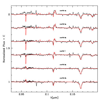
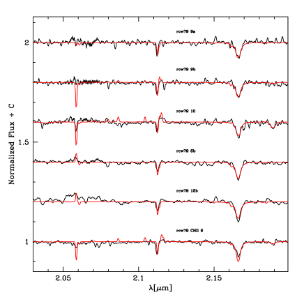
Figure 20: Best CMFGEN fits (red) of RCW 79 ionizing sources spectra (black).

Fig. 20 and 21 shows the best–fit we obtained for the brightest ionizing sources of the three H ii regions. In general, those fits are of good quality. The only important discrepancy in a few stars is the He i 2.056 $\mu$m line which is predicted too strong. However, this line has been shown to be extremely sensitive to line-blanketing (Najarro et al. 1994, 2006). Since our models include only a limited number of elements and since some atomic data for metals remain uncertain (see Najarro et al. 2006), the observed discrepancy is not surprising. The derived parameters for each star are gathered in Table 2.

Fig. 6 shows an example of mass–loss rate determination based on Br$\gamma$ in the case of star RCW79 5a. Reducing $\dot{M}$ produces a deeper absorption line. However, below a value of $3\times 10^{-8}$ M_⊙ yr^-1 the line becomes little sensitive to any change of mass–loss rate. In practice, it is the wind density which is derived in the fitting process. Since it is proportional to $\dot{M}$/$v_{\infty}$  an error on $v_{\infty}$ translates into an error on $\dot{M}$. However, it is very unlikely that our estimates of $v_{\infty}$ are off by more than a factor of 2 (which is already a rather extreme case). Hence, a rather conservative upper limit of $10^{-7}$ M_⊙ yr^-1 (including the uncertainty on $v_{\infty}$ and on the normalization and S/N of the observed spectrum) is determined. Since star RCW79 5a is one of the earliest of our sample, it is expected to show the strongest mass loss rate. Consequently, the upper limit on $\dot{M}$ derived for this star also applies to all other ionizing stars. The upper limits we derive are fully consistent with recent determination of mass loss rates of Galactic O5–9 dwarfs based on optical and UV diagnostics (Bouret et al. 2003; Repolust et al. 2004). Actually, mass loss rates up to two orders of magnitudes smaller are routinely found in late O dwarfs (Martins et al. 2004, 2005b; Marcolino et al. 2009).

We have fitted only the $K$–band part of the observed spectra, but our best fit models yield the complete spectral energy distribution from which one can compute the number of ionizing photons and the ionizing luminosity. The values we derived are listed in columns 10 and 11 of Table 2. Such quantities are important to understand the physics and dynamics of H ii regions (see Sect. 6.1).

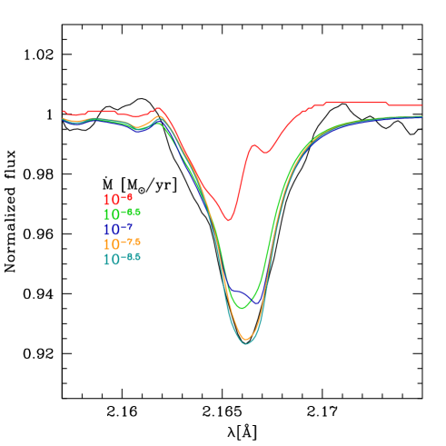
Figure 6: Mass loss estimate for star RCW79 5a. The black solid line is the observed spectrum. The colored lines refer to models with different mass loss rates. A conservative upper limit of $10^{-7}$ M_⊙ yr^-1 is derived.

4.2.2 Age determination

Fig. 7 (left) shows the HR diagram of the ionizing cluster of RCW 79. Evolutionary tracks are from Meynet & Maeder (2003) and include the effects of rotation. All stars lie rather close to the main sequence, on a relatively narrow band, indicating that they most likely formed in a single star formation event. By finding the theoretical isochrone best representing the distribution of stars, the age of the population can be derived. For this, we use the following function:

$$\chi_{iso}^{2}=\sum_{i=1}^{n}\frac{(log(T_{eff}^{i})-log(T_{eff}^{iso}))^{2}}{\sigma^{2}(log(T_{eff}^{i}))}+\frac{(log(L^{i})-log(L^{iso}))^{2}}{\sigma^{2}(log(L^{i}))}$$ (1)

where “iso” stands for “isochrone” and $n$ is the number of stars. $T_{eff}^{iso}$ and $L^{iso}$ are the coordinates of the point of the isochrone closest to the values (T_eff, $L$) representing a star’s position. Hence, $\chi_{iso}^{2}$ is an estimate of the sum over all stars of the distance of a star’s position to the selected isochrone. The isochrone for which this distance is minimized indicates the age of the population. In practice, $\chi_{iso}^{2}$ is evaluated for several isochrones corresponding to ages from 0 to 5 Myr. The results are displayed in Fig. 8. The minimum is found for an age of 2.0–2.5 Myr and a typical uncertainty of $\sim$0.5 Myr. Note that this estimate takes all stars into account. If we use only the five brightest stars, we find a very similar result. This is because the lower part of the HRD is almost insensitive to age due to larger error bars and small separation between isochrones.

The position of the brightest source of the compact H ii region (CHII) on the border of RCW 79 (see Figs. 4 of ZA06 and Fig. 27) is shown by the green triangle in Fig. 7 (left). It is essentially indistinguishable from the position of the ionizing sources. An age estimate for that star would give the same result as for the ionizing sources, within the error bars. The other stars of the CHII region do not help to refine this estimate since they are much fainter and cooler and fall in the region of the HR diagram where the isochrones are tightly packed. Given the errors on the effective temperature and luminosity of star number 6, one can exclude an age younger than 0.5 Myr. This means that if there is any age difference between the CHII region and the ionizing stars of RCW 79 (as would be expected in case of triggered star formation) it is not larger than 2 Myr (see also ZA06).

The right panel of Fig. 7 shows the position of the ionizing stars of RCW 82 and RCW 120. Only the two O stars (e2 and e3) are shown for RCW 82 since we have not analyzed the properties of the Be star e1 (our atmosphere code does not allow a treatment of circumstellar material). Unlike RCW 79, the small number of stars prevents an accurate age determination. Besides, the large uncertainty on T_eff and the relatively low luminosity of the objects (compared to the brightest stars in RCW 79) complicates any attempt to constrain the stars’ age. The only safe conclusion one can draw is that the ionizing stars are younger than 5 Myr. Other than that, any age smaller than 5 Myr is possible.

From interpolation between evolutionary tracks in Fig. 7, one can estimate the masses of the stars of RCW 79. They are summarized in Table 2. Five stars have masses larger than 30M_⊙. If we assume a Salpeter IMF between 0.8 and 100 M_⊙ for the entire population formed with the ionizing sources, one finds a total mass of about 2000M_⊙. Hence, if the star formation event which produced the ionizing stars of RCW 79 also gave birth to lower mass stars, a rather massive cluster was born 2.0–2.5 Myr ago. In that case, the faint sources seen in Fig. 4 are probably intermediate mass main sequence stars born at that time.

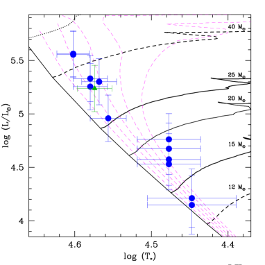
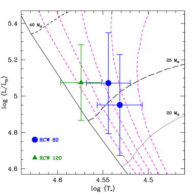
Figure 7: HR diagram of the ionizing sources of RCW 79 (left) and RCW 82 and RCW 120 (right). Evolutionary tracks are from Meynet & Maeder (2003). Isochrones corresponding to ages of 1, 2, 3, 4, 5 Myr are shown by magenta dashed lines. Left: Blue circles are the ionizing stars of RCW 79 and the green triangle is star number 6 in the compact H ii region on the border of RCW 79. Right: the ionizing source of RCW 120 is shown by the green triangle, while the two O stars ionizing RCW 82 (sources e2 and e3) are shown by the blue circles. The Be star (e1) is not shown because its properties have not been derived in our study.

Figure 8: Age estimate of the cluster of the ionizing sources of RCW 79. A value of 2.3$\pm$0.5 Myr is obtained. The solid line is a spline fit curve.

Table 2: Derived stellar properties of the ionizing stars of RCW 79, RCW 82 and RCW 120.

Source	ST	Teff	$\log\frac{L}{L_{\odot}}$	Mevol	log(Q0)	log(L0)
		[kK]		[M⊙]
RCW79 2	O7.5–8V/III	36$\pm$2	4.95$\pm$0.22	$26.2^{+6.1}_{-4.8}$	48.45$\pm$0.23	37.90$\pm$0.23
RCW79 4a	O4–6V/III	40$\pm$2	5.56$\pm$0.22	$46.1^{+13.3}_{-12.7}$	49.25$\pm$0.23	38.74$\pm$0.23
RCW79 5a	O4–6V/III	40$\pm$2	5.56$\pm$0.22	$46.1^{+13.3}_{-12.7}$	49.25$\pm$0.23	38.74$\pm$0.23
RCW79 6a	O6–8V/III	38$\pm$2	5.33$\pm$0.22	$36.2^{+7.2}_{-6.2}$	48.91$\pm$0.23	38.40$\pm$0.23
RCW79 6b	O9–B2V	28$\pm$4	4.15$\pm$0.27	$13.2^{+3.5}_{-3.8}$	47.00$\pm$0.31	36.42$\pm$0.31
RCW79 7	O6–8V/III	37$\pm$2	5.30$\pm$0.22	$35.1^{+6.4}_{-7.3}$	48.80$\pm$0.23	38.28$\pm$0.23
RCW79 8a	O9–B2V/III	30$\pm$3	4.76$\pm$0.24	$19.2^{+5.0}_{-3.7}$	47.33$\pm$0.26	36.75$\pm$0.26
RCW79 8b	O9–B2V/III	30$\pm$3	4.67$\pm$0.24	$18.6^{+4.6}_{-4.2}$	46.75$\pm$0.26	36.16$\pm$0.26
RCW79 9a	O9–B2V/III	30$\pm$3	4.57$\pm$0.24	$17.7^{+4.3}_{-4.4}$	47.95$\pm$0.26	37.38$\pm$0.26
RCW79 9b	O9–B2V/III	30$\pm$3	4.53$\pm$0.24	$17.3^{+4.1}_{-4.5}$	48.52$\pm$0.26	37.99$\pm$0.26
RCW79 10	O6.5–8V/III	38$\pm$2	5.26$\pm$0.21	$34.5^{+6.8}_{-5.9}$	48.96$\pm$0.22	38.45$\pm$0.22
RCW79 12b	O9–B2V/III	28$\pm$4	4.21$\pm$0.27	$13.6^{+3.7}_{-3.8}$	47.06$\pm$0.31	36.48$\pm$0.31
CHII #6	O7.5–9.5V/III	37.5$\pm$2	5.25$\pm$0.22	$34.1^{+6.6}_{-6.8}$	48.79$\pm$0.23	38.26$\pm$0.23
RCW82 e2	O9–B2V/III	34$\pm$2	4.95$\pm$0.27	$24.1^{+6.5}_{-5.0}$	48.37$\pm$0.28	37.81$\pm$0.28
RCW82 e3	O9–B2V/III	35$\pm$2	5.07$\pm$0.27	$27.5^{+8.5}_{-5.8}$	48.59$\pm$0.28	38.05$\pm$0.28
RCW120 e	O6–8V/III	37.5$\pm$2	5.07$\pm$0.21	$29.9^{+5.9}_{-6.8}$	48.58$\pm$0.22	38.05$\pm$0.22

Note 1: The columns are: target name, spectral type, effective temperature, luminosity, evolutionary mass, ionizing flux, ionizing luminosity.
Note 2: The errors on the last two parameters only take into account the uncertainties on T_eff and $\log\frac{L}{L_{\odot}}$.

5 YSOs on the borders of H ii regions

In this section we now focus on the second groups of objects: embedded sources on the borders of the H ii regions. They have been classified as candidate YSOs by ZA06, ZA07, DE09 and PO09. Our aims are the following: 1) confirm spectroscopically the YSO nature of these sources, 2) get more insight into their physical properties (presence of disks, envelopes, jets, outflows). For this, twenty-three YSOs have been observed: 8 around RCW 79, 5 around RCW 82, and 10 around RCW 120. They were selected mainly from their high $K$–band magnitude. Their position and photometry is given in Table 3. Appendix B gives further details on each individual objects. We first present a general description of their spectral properties (Sect. 5.1) before confronting them to near and mid infrared photometry (Sect. 5.2). We then focus on YSOs with strong H₂ emission lines in Sect. 5.3. The morphological and kinematic properties of a few objects are presented in Sect. 5.4 where we show that the YSOs are associated to the HII regions.

5.1 Spectroscopy of embedded sources

The 23 objects we have observed on the borders of the three H ii regions show four main type of spectral signatures: Br$\gamma$ emission, H₂ emission, CO bandheads emission and CO bandheads absorption. Some sources are entirely dominated by one type of spectroscopic signatures, but others can show several features, such as Br$\gamma$ and H₂ emission, or H₂, Br$\gamma$ and CO emission. Table LABEL:tab_specYSOs summarizes the main spectroscopic properties of each source. Their spectra are shown in Figs. 22 and 23. Below, we describe the various sources, grouping them according to the main feature they display.

• H₂ emission sources: ro–vibrational H₂ transitions are observed in these objects. The strongest one is H₂ 1–0S(1) at 2.122 $\mu$m and it is sometimes the only line observed. However, in the majority of “H₂ emission sources” a number of other lines are observed. They are identified on Fig. 22 (top right). Such lines are known to be formed either thermally in shocks (e.g. Burton et al. 1990), or by fluorescence after excitation of H₂ molecules by non ionizing FUV radiation in the Lyman-Werner band (e.g. Black & van Dishoeck 1987). In the latter case, the lines are formed under non LTE conditions. They can thus trace either outflows or photo-dissociation regions (PDRs) in young star forming regions. In Sect. 5.3, we will analyze quantitatively these sources to track the nature of the exciting mechanism.

• Br$\gamma$ emission sources: strong Br$\gamma$ emission is observed in several sources, sometimes in combination with H₂ emission. Br$\gamma$ may have various origins. According to Bik et al. (2006), the large line widths (100–200 km s^-1) could be explained by ionized gas flowing from the surface of a circumstellar rotating disk, rather than a pure nebular origin. Other mechanisms such as accretion flows or outflows are alternative possibilities. In the former case, magnetospheric accretion (van den Ancker 2005) or inner disk accretion (Muzerolle et al. 2004) theoretical models predict Br$\gamma$ emission. For outflows, classical stellar winds, X–winds (Shu et al. 1994) or disk winds (Blandford & Payne 1982, e.g.) lead to ionized hydrogen emission. Interferometric observations of Herbig Ae/Be stars by Kraus et al. (2008) favour Br$\gamma$ emission in extended stellar or disk winds.

• CO bandheads emission sources: CO first overtone emission at 2.2935 $\mu$m (CO(2-1)), 2.3227 $\mu$m (CO(3-1)), 2.3535 $\mu$m (CO(4-2)), 2.3829 $\mu$m (CO(5-3)) is observed in eight sources. This spectral signature has been observed in a number of low and high mass YSOs (Scoville et al. 1979; Chandler et al. 1993; Bik et al. 2006). It is commonly attributed to irradiation of an accretion disk by the central object (Chandler et al. 1995; Kraus et al. 2000). This interpretation is motivated by the temperature (2500 to 5000 K) and density ($n\sim 10^{10-11}$ cm^-3) conditions required to produce such an emission, placing the emitting zone close to the central star (within 0.5 AU for the Be star 51 Oph studied by Berthoud et al. 2007; Tatulli et al. 2008). The geometry of the bandheads depends on the Keplerian rotation and viewing angle. Bik & Thi (2004) used the formalism of Kraus et al. (2000) to show that CO emission in the massive YSOs observed by Bik et al. (2005) was produced in a keplerian disk. Our spectra do not have high enough resolution to detect line asymmetries. In the strongest CO emitters of our sample, Na i 2.206–2.209 $\mu$m and Ca i 2.261–2.264 $\mu$m emission is also detected (see Fig. 22).

• CO bandheads absorption sources: the CO first overtone lines are observed in absorption in a few sources (Fig. 22, bottom right). The line depth ranges from less than 10$\%$ to about 40$\%$ of the continuum.. Na i 2.206–2.209 $\mu$m, Ca i 2.261–2.264 $\mu$m and Mg i 2.281 $\mu$m lines are usually observed in absorption as well. In one object (RCW120 51b) a significant Br$\gamma$ emission is observed, while in another one (RCW82 98) H₂ emission lines are present. CO absorption in the $K$–band is typical of cool stars (red supergiants, AGBs, giants), but it is also detected in YSOs (Casali & Matthews 1992; Hoffmeister et al. 2006; Aspin et al. 2009a). In the latter case, it is thought that CO absorption is observed due to the absence of a strong disk and/or envelope emission which otherwise dominates the $K$–band spectrum and leads to either featureless or emission line spectra. This is consistent with the fact that CO absorption YSOs tend to be class II (and not class I) objects (Casali & Matthews 1992). CO absorption is also observed in the rare class of eruptive FU Orionis objects (FUOr, Reipurth & Aspin 1997). They are thought to be active T–Tauri stars experiencing an accretion burst. Aspin et al. (2009b) collected spectra of V1647 Orionis, the FUOr star responsible for the appearance of the McNeil nebula (McNeil et al. 2004), and show that its CO bandheads shift from absorption to emission when the star experiences a FUOr event. Calvet et al. (1991) explained theoretically this type of transition by an increase of the accretion rate. EXor variables which are pre main sequence objects similar to Fuor stars but with weaker outbursts also display CO absorption bandheads (Lorenzetti et al. 2009).

All these spectral signatures are typical of YSOs. In spite of this general grouping in four categories, we stress again that a few sources share several of these spectral characteristics, highlighting the complexity of the physical phenomena associated with YSOs. In the following, we attempt to better characterize the nature of the sources using infrared photometry.

5.2 Near and mid infrared photometry

All our sources have been observed by 2MASS. We have seen that in the case of the ionizing stars of RCW 79, some 2MASS sources were actually multiple. Similarly, some YSO candidates have been resolved into several sub–components by our SINFONI observations (see Figs. 24, 25 and 30). Hence, the 2MASS photometry is only indicative for those specific sources. Fig. 9 shows a $JHK$ color–color diagram based on 2MASS photometry. Star symbols refers to multiple sources. When available, we have used ESO/NTT/SofI photometry from ZA06, ZA07 and PO09 since it is more accurate and does not suffer from the same uncertainties. The main sequence is also plotted together with A_V=40 mag reddening vectors. The main conclusion is that most of the objects show near–IR excess. Eight objects lie close to the reddening vectors. Out of them, three are multiple sources. Among the five remaining objects, RCW120 C4-64 shows CO absorption bandheads and is most likely a foreground giant star. The near–IR excess observed in the objects far from the reddened main sequence is usually indicative of the presence of an envelope or a disk. It thus confirms that most of our sources are YSOs.

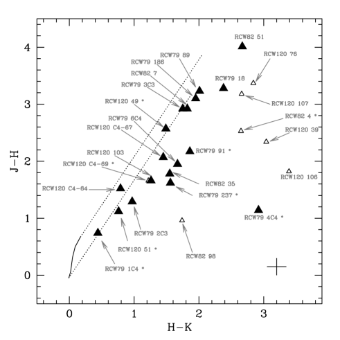
Figure 9: $JHK$ Color-color diagram (magnitudes from 2MASS and NTT-SofI) of the YSOs associated with RCW 79, RCW 82 and RCW 120. The location of main sequence stars is shown by the solid line. Reddening lines have a length corresponding to a visual extinction of 40 mag. Filled (open) triangles correspond to good (uncertain, from 2MASS catalog flag) magnitude measurements. Star symbols following the names indicate multiple sources. The typical error bar of good measurements is indicated.

To get more insight into the nature of the sources, we have retrieved Spitzer/IRAC photometry (when available) from the GLIMPSE survey (Benjamin et al. 2003) to build the color–color diagram shown in Fig. 10. The different symbols correspond to the four spectroscopic groups defined in Sect. 5.1. Class I and II objects gather within the dashed and solid lines respectively. Stars are shown by pentagons close to (0,0).

All our sources fall in the area corresponding to Class I and Class II YSOs. They gather around the color point (0.8, 0.8); some of them may be Class II sources displaced by extinction (see Fig. 10). As discussed by Robitaille et al. (2008) a few of these sources may be extreme AGB stars (see also Srinivasan et al. 2009). It is probably the case of the CO absorption sources RCW120 39 and 64. Four sources have different colors: two are pure H₂ sources (RCW79 237 and 3C3), the two others have colors typical of PDRs (RCW79 1C4, associated with extended 8 $\mu$m and 24 $\mu$m emission, and RCW79 2C3). The two sources with the largest [3.6]$-$[4.5] color are the ones with the strongest H₂ lines (Fig. 22, top right). Smith & Rosen (2005) showed that numerous H₂ lines contributed to the IRAC fluxes, but that the integrated line intensity was the largest in the 4.5 $\mu$m band. Hence, the presence of strong H₂ lines in the $K$–band of RCW79 3C3 and RCW79 237 is probably responsible for an intense emission in the 4.5 $\mu$m band, leading to an increased flux compared to the 3.6 $\mu$m channel. Consequently, the value of [3.6]$-$[4.5] is larger in those two objects, explaining their location in Fig. 10. The other H₂ dominated sources have weaker lines, and consequently their IRAC colors are not affected.

Except for the four cases discussed above, the general conclusion is that objects with similar IRAC colors can present different spectroscopic signatures. Said differently, there is no direct correlation between IRAC colors and a spectroscopic group. Once again, the multiplicity of a few sources complicates the interpretation.

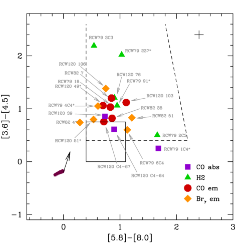
Figure 10: Color–color diagram with SPITZER/IRAC magnitudes of the YSOs associated with RCW 79, RCW 82 and RCW 120. Different symbols are used for the four spectroscopic groups defined in Sect. 5.1: triangles for H₂ sources, squares for CO absorption sources, circles for CO emission sources and diamonds for Br$\gamma$ dominated sources. Pentagons indicate main sequence massive stars (from Martins et al. 2005a). Colors of class II (respectively I) sources are delineated by solid (resp. dashed) lines according to Allen et al. (2004). The reddening vector shown by the black arrow is computed for a visual extinction of 40 magnitudes with the law of Indebetouw et al. (2005). Star symbols following source names indicate multiple sources.

Fig. 11 shows a color–magnitude diagram based on Spitzer/MIPS 24 $\mu$m photometry (Carey et al. 2009), complemented by AKARI observations (Zavagno et al. in prep). The magnitude in this band corrected for the distance modulus of each source (noted [24]_dc), is plotted as a function of $K-$[24]. For comparison, the theoretical SEDs of Martins et al. (2005a) have been used to calculate the positions of O stars in this diagram. They are shown by the pentagon symbols. A reddening vector corresponding to A_V=40 mag and to the extinction law of Lutz (1999) is indicated. All YSOs are brighter at 24 $\mu$m and much redder (in $K-$[24]) than O stars. This indicates once more that they have a strong infrared excess due to envelopes and/or disks which dominate the SED at those wavelengths. The H₂ sources seem to stand out in this diagram. While most sources are grouped in a region defined by -12 $<$ [24]_dc $<$ -6 and 7 $<$ $K-$[24] $<$ 10, four out of the five H₂ sources for which infrared photometry is available are much brighter and redder ([24]_dc $<$ -12 and $K-$[24] $>$ 10). This might be an indication that those objects have larger amount of circumstellar material tracing an earlier state of evolution, or that they have larger masses.

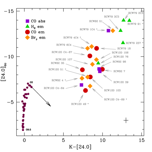
Figure 11: Color–magnitude diagram with SPITZER/MIPS 24 $\mu$m magnitudes of the YSOs associated with RCW 79, RCW 82 and RCW 120. On the Y axis, the magnitudes have been corrected for distance. The symbols have the same meaning as in Fig. 10. The arrow indicates an extinction of A_V=40 magnitudes (law of Lutz 1999). The pentagons are O stars from the theoretical SEDs of Martins et al. (2005a). Star symbols following source names indicate multiple sources.

This is confirmed by Fig. 12 showing the [3.6]$-$[5.8] vs [8.0]$-$[24] diagram. Here again, the H₂ objects are clearly located towards redder colors (with the exception of RCW120 76). The solid lines delineates the location of stage I and II objects of Robitaille et al. (2006). This classification is the theoretical analog of class I and II sources, meaning that stage I objects correspond to models with an envelope, while stage II sources have disks and possibly a tenuous envelope. H₂ sources are therefore consistent with being stage I objects as suspected previously. The bulk of the other objects are again located in the transition region between stage I and stage II sources. Only RCW120 51 and RCW82 51 might appear as stage I objects. We will discuss further these results in Sect. 6.2 using additional findings presented below.

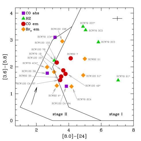
Figure 12: [3.6]$-$[5.8] vs [8.0]$-$[24] diagram. The symbols have the same meaning as in Fig. 10. The arrow indicates an extinction of A_V=40 magnitudes. The solid lines delineates the areas where stage I and II objects of Robitaille et al. (2006) are found (see their Fig. 23). Star symbols following source names indicate multiple sources.

The main conclusion of this analysis of color–color and color–magnitude diagrams is that the objects dominated by H₂ emission seem to be different from the remaining of the sources we observed. They probably have an optically thick envelope. The other objects are more consistent with YSO surrounded by disks. Another conclusion regarding these sources is that they can have different spectroscopic signatures but similar colors. This can be partly explained by geometrical effects. Indeed, depending on the inclination and size of the putative disks, different regions are visible, and thus different spectral lines are expected. The corresponding photometry is also modified. Whitney et al. (2003b, a) showed that in the [3.6]$-$[4.5] vs [5.8]$-$[8.0], a spread of about one magnitude can be expected due to inclination effects. This corresponds to what we observe. Hence, among the CO emitters, absorbers and Br$\gamma$ emitters, one probably sees a population of class II objects at different inclinations.

Table 3: 2MASS and NTT/SofI $JHK$, Spitzer-GLIMPSE, Spitzer-MIPS and AKARI magnitudes of YSOs.

Star	RA	DEC	$J$	$H$	$K_{\rm{S}}$	[3.6]	[4.5]	[5.8]	[8.0]	[24]	nature
	h m s	${}^{\circ}\arcmin\ \arcsec$
YSOs around RCW 79
237	13:41:02.3	-61:44:16	17.41	15.79	14.23	11.02	9.00	7.52	6.49	1.61a	Class I
91	13:40:57.6	-61:45:44	16.62	14.45	12.59	8.66b	7.60b	7.16	6.21	-0.84a	Class I
18	13:40:58.3	-61:46:50	17.11	13.83	11.45	8.57	7.54	6.70	5.87	2.21	Class I
89	13:40:59.0	-61:46:51	18.58	15.35	13.34	10.83	10.71	–	–	–	–
186	13:40:58.5	-61:46:48	18.96	15.86	13.91	–	–	–	–	–	–
2C3	13:40:32.7	-61:47:20	14.08	12.79	11.82	9.54	9.04	6.62	4.96	-0.87a	Class I
3C3	13:40:26.6	-61:47:56	17.24	14.32	12.57	9.21	7.02	5.84	5.30	0.26a	Class I
1C4	13:39:53.6	-61:41:21	12.19	11.45	11.01	8.19b	7.94b	5.09b	3.41b	0.26a	–
4C4	13:39:55.9	-61:40:58	14.68	13.54	10.62	7.27	6.22b	5.28	4.67	2.01b	Class I
6C4	13:40:08.9	-61:41:38	13.91	11.96	10.29	8.78	8.18	7.51	6.38	2.21a	Class I
YSOs around RCW 82
4	13:59:34.8	-61:19:22	17.59:	15.06	12.41	9.89	9.15	8.59	8.30	5.04	Class I
7	13:59:47.3	-61:22:02	18.77c	15.85c	14.03c	11.34	10.14	9.02	8.17	4.05	Class I
35	13:59:50.9	-61:25:22	14.29	12.51	10.96	8.61	7.79	6.97	6.11	2.58	Class I
51	13:59:57.6	-61:24:37	17.81c	13.80c	11.13c	8.31	7.48	6.01	4.80	-0.19	Class I
98	13:59:36.7	-61:20:48	16.27:	15.31:	13.57	10.09	9.24	8.47	–	4.01	–
YSOs around RCW 120
39	17:12:00.9	-38:31:40	17.29:	14.95:	11.91	7.43	6.57	5.66	4.93	2.26	Class II
49	17:12:08.0	-38:30:52	16.24	13.67	12.18	10.59	9.53	8.85	8.16	4.36	Class I/II
51	17:12:28.5	-38:30:49	12.85	11.73	10.97	10.00	9.20	8.31	7.78	2.88	Class I/II
C4-64	17:12:40.8	-38:27:29	13.37	11.85	11.06	9.78	9.17	8.50	7.60	3.75	Class I/II
C4-67	17:12:41.1	-38:27:17	13.03	10.96	9.51	7.78	7.03	6.27	5.56	2.09	Class I/II
C4-69	17:12:42.2	-38:26:58	15.16:	13.50	12.28	10.82	9.75	8.78	–	3.87	Class I/II
76	17:12:46.0	-38:25:25	17.03:	13.66	10.82	7.61	6.40	5.37	4.47	1.37	Class I/II
103	17:12:40.2	-38:20:31	14.23	12.57	11.31	9.40	8.29	7.24	6.13	2.87	Class I/II
106	17:11:50.7	-38:19:55	17.62:	15.80:	12.41	8.27	6.89	5.79	4.95	0.97	Class I
107	17:12:33.6	-38:19:52	16.03:	12.85	10.19	7.13	–	5.32	4.57	1.48	Class I/II

Note: Classification into class I/II objects is from ZA06, PO09, DE09. The notation “:” uncertain flux measurements due to the weakness of the source. The typical errors are 0.1 mag (respectively 0.3 mag) for IRAC (resp. MIPS) photometry.
^a AKARI magnitude
^b Magnitude obtained by aperture photometry (see ZAV05)
^c NTT magnitude

Table 4: Characteristics of the YSO spectra. When present, lines are in emission unless stated differently.

Source	Br$\gamma$	H2	CO	Notes
YSOs around RCW 79
237	no	2.0338, 2.1218, 2.2233, 2.2477	no
237-b	no	no	absorption	Na i, Ca i absorption
91	yes	2.0338, 2.1218, 2.2233	no
91-a	yes	2.033, 2.1509	emission
91-b	yes	1.9576, 2.0338, 2.1218, 2.2233	weak emission
18	yes	no	emission	Na i emission
186	yes	no	no	$+$3198
89	yes, weak	no	no
2C3	yes, on top of absorption	2.0338, 2.1218, 2.2233	no
3C3	yes, weak	2.0338, 2.1218, 2.2233, 2.2477	no
3C3-b,c,d	no	2.1218	no
1C4	yes, absorption	no	absorption	Na i, Ca i absorption. PDR associated with this objet
4C4	yes, weak	no	no	faint companions
6C4	yes	no	no
YSOs around RCW 82
4	yes	no	no
7	?	1.9576, 2.0338, 2.1218, 2.2233	emission
35	yes	2.0338, 2.1218, 2.2233	emission	Na i emission
51	yes	2.0338, 2.1218	emission (weak)
98	no	1.9576, 2.0338, 2.1218, 2.2233, 2.4066, 2.4134	absorption	H2 lines probably not related to YSO, see Fig. 24
YSOs around RCW 120
39	no	no	absorption	Na i, Ca i absorption
49	yes	2.0338, 2.1218, 2.2233, 2.2477	emission
49-a	no	2.0338, 2.1218, 2.2233	absorption
49-b	no	2.0338, 2.1218, 2.2233	absorption?
51-a	yes	no	no
51-b	no	no	absorption
51-c	no	no	absorption	Na i, Ca i absorption
C4-64	absorption	no	absorption	Na i, Ca i absorption
C4-67	yes	2.1218	emission
C4-69a	no	no	no	featureless
C4-69b	yes	no	absorption
C4-69c	no	no	absorption	Na i, Ca i absorption
C4 A	absorption	no	absorption	PDR associated with this object
C4 Ba	absorption	no	no	PDR associated with this objet
C4 Bb	no	no	absorption	Na i, Ca i absorption
76	no	2.0338, 2.1218, 2.2233	no
103	yes	1.9576, 2.0338, 2.1218, 2.2233, 2.4066, 2.4237	emission	Na i, Ca i emission
106	yes	no	no
107	yes, weak	2.0338, 2.1218, 2.2233	no

5.3 Nature of H₂ sources

Several sources observed on the border of the H ii regions show H₂–dominated spectra (see top right panel of Fig. 22 for line identification). As described in Sect. 5.1, H₂ emission is due either to thermal processes or to fluorescence. The relative intensity of individual lines is different in either cases. Comparing H₂ line strength can thus lead to the underlying excitation mechanism. For a thorough comparison, line fluxes must be dereddened, which requires the knowledge of extinction. This piece of information is difficult to obtain since the intrinsic SED of our sources is not known. From Fig. 9 one can see that most objects have a visual extinction in the range 10–40 mag. We have thus adopted a typical extinction A_K = 2.5$\pm$1.5 for the present study. We used the Galactic extinction law $\propto\lambda^{-1.7}$ similar to Moneti et al. (2001) to deredden the line fluxes.

Figure 13: H₂ excitation diagram of the sources showing H₂ emission spectra (either pure or mixed with other spectral features). All N/g numbers are relative to N/g for transition 1-0S(1). The solid line are fits to the $\nu=1$ level populations assuming LTE and A_K=2.5. The corresponding temperature is indicated for each YSO. The dotted lines are fits for the cases where A_K=1.0 and A_K=4.0. The error bars take into account measurement errors and an uncertainty of $\pm$1.5 in A_K.

We have computed the column densities $N_{i}$ of several excited levels and plotted them as a function of level energy $E_{i}$. This has been shown to be a powerful tool to distinguish between thermal and radiative emission (e.g. Hasegawa et al. 1987). If H₂ emission is thermal, the values of $N_{i}/g_{i}$ ($g_{i}$ being the statistical weight) follow a Boltzmann distribution and are thus aligned in a $log(N_{i}/g_{i})-E_{i}$ diagram. Alternatively, radiative pumping should increase the population of high energy levels and introduce a departure from linearity in the aforementioned diagram. We have computed the column densities of several levels using the same formalism and molecular data as Martín-Hernández et al. (2008). Our results are shown in Figs. 13. The solid and dotted lines correspond to a linear fit of the $\nu=1$ levels. The slope is directly related to the temperature of the Boltzmann distribution best representing these energy levels. Solid lines are for the case $A_{K}$=2.5, while the dotted lines are for $A_{K}$=1.0 and $A_{K}$=4.0. When extinction varies, line fluxes are affected, which explains the different slopes for different $A_{K}$. From Fig. 13 RCW79 3C3, RCW120 103 and RCW79 91b appear consistent with pure thermal emission. For RCW 79 2C3, RCW120 76, RCW120 49 and RCW120 107, a marginal deviation from pure thermal emission is found, although the bulk of the emission seems to be thermal. Source RCW82 7 shows too few lines to draw any final conclusion. Besides, we will see in Sect. 5.4 that H₂ emission is much extended and patchy. Finally, RCW79 237 clearly shows a significant non thermal contribution.

Two more sources (RCW79 89 and RCW79 91) display H₂ lines, but not enough to build excitation diagrams. For these sources, we calculated the ratios $\frac{I_{1-0s(1)}}{I_{2-1S(1)}}$ and $\phi_{1}$ (defined by Smith et al. 1997). Under LTE conditions, the first ratio should have values between 5 and 100 (for temperatures ranging between 3000 and 1000 K respectively, see Gustafsson et al. 2008), and the second ratio should be close to 3. When fluorescence dominates, lower values are expected. For RCW79 89, the observed values are 4.61$\pm$0.79 and 2.89$\pm$0.56 respectively, indicating that H₂ has probably multiple origins. For RCW79 91, FUV excitation is clearly favored since $\frac{I_{1-0s(1)}}{I_{2-1S(1)}}$ = 6.33$\pm$0.14 and $\phi_{1}$ = 0.99$\pm$0.14.

In conclusion, most sources show a thermal H₂ spectrum with, in some cases, a possible contribution from fluorescence. Three sources (RCW79 237, RCW79 89 and RCW79 91) are probably dominated by non thermal emission, most likely due to the presence of nearby PDRs. Thermal emission is usually attributed to shocks. Davies et al. (2000) summarized the various types of shocks encountered in the ISM using the models of Burton et al. (1990). They note in particular that fast J–shocks are usually dissociative. In that case, molecules are formed on grains in the post-shock region and are produced in excited states. Consequently, their emission spectrum is more typical of a non-thermal mechanism since the molecules will cascade down to lower energy levels. Hence, fast J–shocks seem to be excluded to explain the thermal emission of most of our H₂ sources. Similarly, slow C–shocks are not favored either since they are associated with rather low temperatures ($<$300 K). From Fig 13 we see that temperatures of 1000–2500 K are estimated, inconsistent with slow C–shocks. Hence, slow J–shocks or fast C–shocks, both heating the gas to 2000–3000 K, are preferred to account for the observed thermal H₂ emission in our sources.

5.4 Morphology and kinematics of selected YSOs

In this section we gather information on the morphology and kinematics of some YSOs in order to study their physical association with the H ii regions and to get more insight into the origin of the observed emission lines.

We first focus on the kinematics of the YSOs themselves. The emission lines of their spectra (Br$\gamma$ and/or H₂) have been fitted by 1D Gaussians using QFitsView. We have first measured the full width at half maximum (FWHM) of the sky lines to estimate the spectral resolution of the observations. We obtain FWHM$=84\pm 6$ km s^-1, thus a resolution R$=3575\pm 250$. Then we have measured the central positions and the widths of the H₂ and Br$\gamma$ lines (only for the lines presenting a good signal to noise ratio). These quantities are given in Table 5. The first and second columns identify the YSO; the indication “ext” means that we have measured the nebulous extended emission in the vicinity of the YSO. The following columns give, for a selection of lines, the LSR velocity ($V_{\rm LSR}$) and the intrinsic line width ($\Delta V$). The absence of measurement for some lines is due to the poor quality of the data at hand. We estimate that the uncertainty on $V_{\rm LSR}$ is $\sim 10$ km s^-1. The relative uncertainty on the measured line widths if of 10$\%$, but the uncertainty on $\Delta V$ is large. Its is about 20 (40) km s^-1 for wide (narrow) lines. This is mainly due to the large uncertainty on the instrumental width. Hence, values given in Table 5 are only indicative.

Table 5: Velocity measurements. For each line, the first value is the LSR radial velocity while the second value (in parenthesis) is the line width.

Region	source	Br$\gamma$	H2 1.9576	H2 2.0338	H2 2.1218	H2 2.2233	H2 2.4066	H2 2.4237
RCW 79	18	-58 (196)	– –	– –	– –	– –	– –	– –
	91	-75 (202)	– –	– –	-57 (60)	-56 (–)	– –	– –
	91a	-63 (152)	– –	– –	– –	– –	– –	– –
	91b	– –	– –	– –	-58 (72)	-56 (80)	– –	– –
	237 ext	-57 (–)	– –	– –	-53 (–)	– –	– –	– –
	237	– –	– –	-62 (83)	-60 (78)	-62 (–)	-59 (63)	-56 (75)
	1C4	-49 (–)	– –	– –	-46 (–)	– –	– –	– –
	2C3	– –	– –	-43 (–)	-45 (33)	-46 (nr)	-44 (nr)	-45 (nr)
	3C3	– –	-95 (95)	-80 (103)	-79 (88)	-76 (75)	-79 (84)	-77 (76)
	3C3 bow	– –	-88 (–)	-73 (–)	-72 (72)	-71 (70)	-67 (50)	-69 (49)
	CHII	-42 (–)	– –	– –	-49 (–)	– –	– –	– –
RCW 82	4	-52 (228)	– –	– –	– –	– –	– –	– –
	7 ext	– –	– –	– –	-56 (43)	– –	– –	– –
	35	-50 (209)	– –	– –	-100 (188)	– –	– –	– –
	51 ext	– –	– –	– –	-56 (nr)	– –	– –	– –
	51	-74 (181)	– –	– –	-59 (66)	– –	– –	– –
	98	– –	– –	-57 (–)	-55 (69)	-56 (–)	-47 (45)	-51 (nr)
RCW 120	49	-29 (162)	– –	– –	-30 (142)	– –	– –	– –
	51 ext	-10 (–)	– –	– –	– –	– –	– –	– –
	51	-5 (162)	– –	– –	– –	– –	– –	– –
	76	– –	– –	-30 (–)	-28 (78)	– –	– –	– –
	103	-12 (137)	-67 (–)	-74 (–)	-79 (111)	-76 (–)	– –	– –
	107	-30 (171)	– –	– –	– (103)	– –	– –	– –

Note: All velocities are in km s^-1. The notation “nr” stands for “not resolved” and “ext” refers to extended emission.

The $V_{\rm LSR}$ velocities can be compared to the $V_{\rm LSR}$ velocities of the ionized gas and associated molecular material. These velocities are in the ranges $-52$/$-46$ km s^-1 for RCW 79 (ZA06), $-52$/$-42$ km s^-1 for RCW 82 (PO09), and $-14$/$-8$ km s^-1 for RCW 120 (ZA07). The comparison shows that (and taking into account the uncertainty on the velocity):

• the YSOs velocities in RCW 79 are in rather good agreement with those of the H ii region, except for 3C3. In this YSO the H₂ gas approaches us with a velocity of the order of 30 km s^-1. 3C3 has a nearby extended structure (a bow-arc like structure, see Fig. 24) presenting the same velocity.

• the YSOs in RCW 82 have velocities comparable to those of the associated region; an exception is source 35 with very different velocities for the H₂ and Br$\gamma$ lines. The H₂ material approaches us with a velocity $\sim$50 km s^-1 with respect to the material emitting the Br$\gamma$ line and the RCW 82 region.

• in RCW 120, YSO #51 has a velocity comparable to that of the H ii region; it is the only one (see also below). YSOs #49, #76, and #107 are approaching us with a velocity of about 20 km s^-1. The situation is worse for YSO #103, and resembles very much that of source 35 in RCW 82: the Br$\gamma$ line has the same velocity as the RCW 120 region, whereas all the H₂ lines show an approach velocity of some 50–60 km s^-1. This may be indicative of flows (see below), but may also suggest that these YSOs are not associated with RCW 120. We do not favor this last solution as these three YSOs are observed in the direction of well defined condensations in the shell of dense neutral material interacting with the ionized region. Molecular observations of this shell (allowing velocity measurements) should help to clarify this point.

Table 5 shows another interesting feature: the Br$\gamma$ emission lines are wide (up to 200 km s^-1), and always wider than the H₂ lines. This again probably indicates that they do not originate from the same zones of the YSOs.

These results indicate that the geometry of the YSO is rather complex, at least in some cases. One can gain further insight into those properties by looking at emission maps and velocity maps. Fig. 14 to 16 show some illustrations. In those figures, the contours of the integrated $K$–band emission are shown on top of images centered on Br$\gamma$ and/or H₂ 2.12 $\mu$memission lines (and from which the continuum is subtracted). Velocity maps built from H₂ 2.12 $\mu$m are also shown when they could be extracted from the data. The main conclusion regarding morphology is twofold: 1) Br$\gamma$ emission is always centered on the emission peak of the integrated $K$–band image, i.e. it coincides with the position of the YSO; 2) H₂ 2.12 $\mu$m is emitted on a much wider scale, with emission peaks sometimes not corresponding to the position of the YSO. Three YSOs have been selected to illustrate these results, but they can be generalized to all YSOs (see appendix B).

The case of RCW120 51 is spectacular. The main $K$–band source in this region is 51a (see Fig. 14). Its spectrum is dominated by Br$\gamma$ (Fig. 22) and Fig. 14 confirms that is is the main emitter in this line. However, we note the presence of a Br$\gamma$ “cone” pointing towards 51a and, more generally, towards the center of the H ii region. This structure is very typical of the ionization front in the vicinity of RCW120 51. Measurements of the radial velocity along this cone ($\sim$ -6 km s^-1) indicates values similar to that of 51a and to that of the H ii region. Hence the YSO and the Br$\gamma$ cone are physically associated, and are also adjacent to the ionization front. The H₂ map of Fig. 14 shows the existence of another emission cone, the orientation of which is the same as that of the Br$\gamma$ emission cone. However its top is not located on source 51a, but rather on a faint $K$–band source located south and east of it (see Fig. 14). The H₂ velocities along this cone are also consistent with those of the H ii region. We are thus directly probing the structure of the ionization front: seen from the H ii region, the line of sight crosses first a Br$\gamma$ cone tracing the ionized gas behind which is located the H₂ cone located closer to the PDR and the molecular material. Along this H₂ cone structure, we measure a ratio $\frac{I_{1-0s(1)}}{I_{2-1S(1)}}$ (respectively $\frac{I_{1-0s(1)}}{I_{3-2S(3)}}$) of 6.2$\pm$0.1 (respectively 12.0$\pm$0.1) intermediate between pure thermal emission and radiative excitation. The presence of non-thermal emission is consistent with the proximity to the PDR. All in all, we have thus a direct proof that the YSO RCW120 51a is located on the ionization front.

For YSO RCW82 7, Fig. 15 shows again that H₂ is emitted over a wider region than the $K$–band continuum. The H₂ emission is not centered on the YSO, but is offset to the west. In addition, diffuse emission concentrations are clearly visible especially north-east of the YSO. The H₂ velocity map constructed by fitting a Gaussian to the 2.12 $\mu$m line reveals that this blob has a radial velocity of -10 km s^-1 compared to -60 km s^-1 for the YSO . This may very well be the signature of a jet centered on the YSO and interacting with molecular gas at the position of the blob. At the distance of RCW 82, such a jet would have a projected length (YSO–blob) of $\sim$0.06 pc. Besides this peculiar H₂ emission, there is an arc–like H₂ structure extending North and South of the YSO. Its velocity is comparable to that of the YSO and to that of the H ii region (see above). It may thus correspond to the PDR on top of which the YSO is located. A similar morphology is identified in RCW120 49 (Fig. 28) and RCW120 103 (Fig. 29), albeit with a lower significance (see Sect. B.3). Another convincing evidence for the presence of a jet comes from YSO RCW120 C4-67. It features a spectacular H₂ map with an arc structure a few arcseconds away from the YSO (see Fig. 16). Its radial velocity is comparable to that of the YSO, but the fact that the arc curvature is directed towards the YSO suggests that it might result from the interaction of a jet and molecular material. It may also be material ejected by the YSO in the past.

From the analysis of the morphology and kinematics of a few sources, we conclude that, in some cases, we have been able to firmly establish the association of the YSO with the ionization front, strengthening the case of triggered star formation. We have also discovered the presence of a possible outflow in RCW82 7 traced by a H₂ velocity gradient (and possibly also in RCW120 49 and RCW120 103). The geometry of the H₂ emission in RCW120 C4-67 is also suggestive of the presence of a jet.

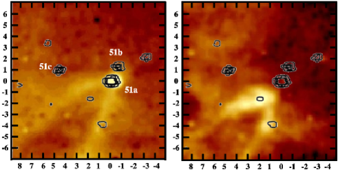
Figure 14: Morphology of RCW120 51. Left panel: Br$\gamma$ emission map. Right panel: H₂ emission map. The contours of the full K–band emission are overplotted. All images have been created from the initial datacubes smoothed with a spatial Gaussian (FWHM = 3 pixels). North is up, East is to the left. The axis indicate the offsets (in arscseconds) relative to the main YSO position (coordinates given in Table LABEL:tab_yso).

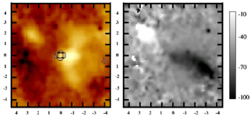
Figure 15: Morphology and dynamics of RCW82 7. Left panel: H₂ emission map together with contours of the full K–band emission. Right panel: H₂ 2.12 $\mu$m velocity map (scale in km s^-1). North is up, East is to the left. The axis indicate the offsets (in arscseconds) relative to the YSO position (coordinates given in Table LABEL:tab_yso).

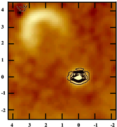
Figure 16: Morphology of RCW120 C4-67. The image shows the H₂ emission map (created from the initial datacubes smoothed with a spatial Gaussian – FWHM = 3 pixels). Contours of the full K–band emission are overplotted. North is up, East is to the left. The axis indicate the offsets (in arscseconds) relative to the YSO position (coordinates given in Table LABEL:tab_yso).

6 Discussion

6.1 Winds and bubbles

The evolution of an H ii region is governed by the ionizing radiation emitted by its ionizing stars – see for example the first order analysis of Dyson & Williams (1997) of the evolution of an H ii region in an homogeneous medium. But it may also be influenced and even dominated by the action of the wind emitted by the central massive star (Freyer et al. 2003). It is often claimed that the many bubbles observed at all scales in the Galactic plane result from the action of such powerful winds (Churchwell et al. 2006). While this is most likely the case when Wolf–Rayet stars are involved (Garcia-Segura & Mac Low 1995; Brighenti & D’Ercole 1997), the dominance of wind effects in the early evolution of interstellar bubbles remains to be established. This is even more true since the recent downward revision of the mass loss rates of O stars due to clumping (e.g. Bouret et al. 2005; Fullerton et al. 2006).

Capriotti & Kozminski (2001) and Freyer et al. (2003) have developed analytical models and hydrodynamical simulations of H ii regions with winds. At the beginning of its evolution, a young H ii region should not be too much affected by the wind emitted by its ionizing star, if any. With time, the stellar wind gets stronger and eventually leads to the formation of a central cavity filled with very hot (T$\sim 10^{6}$ K) low density, shocked gas. This gas emits at X–ray wavelengths. Such an extended X–ray emission is a strong indirect evidence for winds. It has been observed only in the direction of three H ii regions though: M17 (Townsley et al. 2003; Povich et al. 2007), the Rosette nebula (Townsley et al. 2003), and the Orion nebula (Güdel et al. 2008). All regions lie relatively nearby (0.5 to 2 kpc), which might explain that their X–ray emission is more easily detected than in distant regions. They are excited by a cluster of several O stars and have ages ranging from 1 (Orion) to about 3–4 Myr (M17 and Rosette). All three clusters contain early O stars (spectral types O4–O6) with moderately strong winds (compared to early O type supergiants which have larger mass loss rates). This is similar to the three H ii regions we have studied. We do not know if the extended X–ray emission is a common phenomena among bubbles or if it is due to the very massive stellar content of these regions. Unfortunately, RCW 79, RCW 82 and RCW 120 have not been observed at X–ray wavelengths so the effects of winds in the H ii regions cannot be quantified directly.

Dust emission at 24 $\mu$m may be another indicator of the effects of winds. Very small grains, heated by the stellar radiation and out of thermal equilibrium, radiate at 24 $\mu$m (Jones et al. 1999). As long as such emission is observed, it means that dust has not (yet) been swept-up by the stellar winds. The presence of a central hole in Spitzer–MIPS 24 $\mu$m emission maps of some H ii regions might be an indication that winds are at work (Watson et al. 2008). Such a cavity could also be attributed to the radiation pressure of the central exciting stars or to dust destruction by the stars’ ionizing radiation (Inoue 2002; Krumholz & Matzner 2009). However Krumholtz & Matzner show that radiation pressure is generally unimportant for H ii regions driven by a handful of massive stars (thus for our three regions). In any case if a shell is observed at 24 $\mu$m, it means that stellar winds have not removed all the dust from the H ii region. Fig. 17 shows a composite image for the three H ii regions studied here, with red, green and blue being respectively 24 $\mu$m, 3.6$\mu$m and H$\alpha$ emission. The 24 $\mu$m emission traces the hot dust. In all three regions, one clearly sees the presence of 24 $\mu$m emission bows surrounding the ionizing stars. The hot dust very close to those stars is thus either blown away or destroyed by the intense UV radiation. But 5″ to 30″ away, i.e. well within the borders of the H ii regions, dust is detected. Hence, stellar winds have not (yet) removed all dust from the cavities, indicating that their effect on the dynamics of the H ii regions is rather limited.

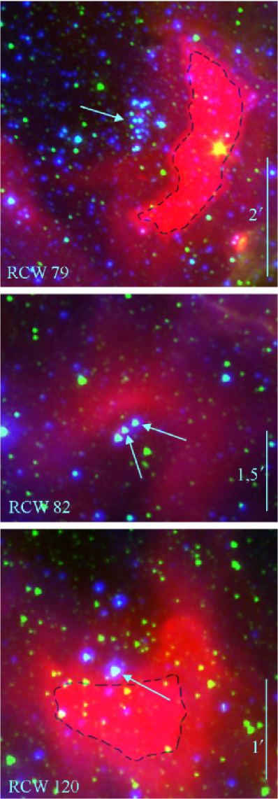
Figure 17: Composite color image around the ionizing stars or cluster in the three H ii regions: red is the Spitzer-MIPSGAL emission at 24 $\mu$m, green is the Spitzer-GLIMPSE emission at 3.6 $\mu$m, and blue is the H$\alpha$ emission. The black dashed line encloses the zones where the 24 $\mu$m emission is saturated. North is up and east is left. The ionizing star(s) or cluster lie in the centre of the H ii regions, in a zone void of dust emitting at 24 $\mu$m. They are indicated by blue arrows.

To better assert the role of stellar winds and radiation in our objects, we focus on RCW 79. Since it hosts the largest number of ionizing stars of the three regions, it is the most appropriate to analyze the influence of stellar winds.

The total number of ionizing photons emitted by the ionizing stars is $10^{49.82}$s^-1 (see Table 2). This corresponds to an ionizing luminosity of $10^{39.31}$ erg s^-1. For an age of the population of 2.3 Myr, the ionizing energy released in the H ii region is thus $10^{53.17}$ erg. In the previous estimate we have assumed that the ionizing luminosity was constant with time. Since the stars are rather young and close to the main sequence, this is a reasonable approximation. According to the Geneva tracks, a 40 M_⊙ star has T_eff = 42560 K and $\log\frac{L}{L_{\odot}}$ = 5.34 on the ZAMS, and T_eff = 39170 K and $\log\frac{L}{L_{\odot}}$ = 5.45 after 2.3 Myr. For the corresponding radius and using the number of ionizing photons per unit area ($q_{0}$) from Martins et al. (2005a), the values of $Q_{0}$ (total ionizing photon flux) are $10^{49.12}$ and $10^{49.16}$ at 0 and 2.3 Myr respectively. Hence our assumption is justified.

The total wind mechanical luminosity at 2.3 Myr is $10^{36.18}$ erg s^-1 (for 12 O stars with a mass loss rate of $10^{-7}$ M_⊙ yr^-1 and a terminal velocity of 2000 km s^-1). Assuming again that this value is constant between 0 and 2.3 Myr, one estimate a total wind mechanical energy release of $10^{50.04}$ erg. To check the validity of our assumption, one can use the scaling relations of Vink et al. (2001) (their Eq. 24). Using the properties of a 40 M_⊙ star on the ZAMS and after 2.3 Myr of evolution (using once more the tracks of Meynet & Maeder 2005), one finds a mass loss rate difference of 0.3 dex. Hence, our wind mechanical energy determination is at the very most overestimated by a factor 2.

The 2D simulations of Freyer et al. (2003, 2006) tackled the question of the effects of winds on the dynamics of H ii regions. They showed that the presence of the wind triggered the formation of structures (“fingers”) in the H ii regions, modifying the efficiencies of energy transfer (from stellar ionizing and wind mechanical energies to ionizing, kinetic and thermal energies in the H ii region). In their simulations, the ratio of ionizing to wind mechanical luminosities was of the order 100. They showed that in spite of this, winds could significantly affect the evolution of the H ii region. In our case, this ratio is at least 1000 (recall that our estimates of mass loss rates are upper limits). The main reason is that although the ionizing luminosities we find are similar to the ones used by Freyer et al., our mass loss rates are lower by nearly a factor of 10. The reason is the inclusion of clumping in our models. It is well known to lead to a downward revision of mass loss rates of O stars (e.g. Hillier 1991). The values of $\dot{M}$ used by Freyer et al. were derived with homogeneous models and are thus higher than our determinations. With this increase by at least a factor of 10 in the ratio of ionizing to wind mechanical luminosity, one might thus wonder whether winds still play a role. The evidence brought by the presence of 24 $\mu$m dust emission argues against a strong effect of stellar winds (at least in the first 2–3 Myrs). New dedicated simulations with reduced mass loss rates are encouraged to shed more light on this issue.

6.2 YSOs: a possible spectroscopic evolution

Among the YSOs observed on the borders of the three H ii regions, a few have a $K$–band spectrum entirely dominated by H₂ emission. We have seen in Sect. 5.3 that thermal emission due to shocks was favored to explain the different line ratios. Besides, most of these sources tend to be brighter and redder in the [24] vs $K$–[24] diagram, indicating a larger amount of circumstellar material (Sect. 5.2) than for the other observed YSOs. All in all, this tends to favour a picture according to which the H₂ sources are in a relatively early phase of evolution. The large 24 $\mu$m emission combined to the absence of direct indicator of the presence of a disk suggests that these sources still possess large envelopes. The H₂ emission probably comes from either a jet–like structure interacting with this circumstellar material, or from an expanding shock created by stellar/disk wind and/or radiation pressure inside the envelope. One can further speculate that objects showing both H₂ lines and other features (Br$\gamma$ or CO bandheads emission) represent later stages of evolution in which the envelope partially disappeared, revealing the disk features. Their somewhat lower reddening and brightness in the [24] vs $K$–[24] diagram lend support to this hypothesis. In that case, both Br$\gamma$ and CO emission could be produced in disks irradiated by the nascent star, Br$\gamma$ being emitted on the surface and CO close to the disk midplane, in zones shielded from UV flux. This could explain that the H₂ lines are usually narrower than Br$\gamma$ in YSOs when both types of lines are detected (Table 5). The latter being emitted on the disk’s surface, it would be rotationally broadened, while the former would reflect the shock conditions in the dissolving envelope. We noted in Sect. 5.4 that a couple of objects showed radial velocities different for Br$\gamma$ and H₂. In the suggested scenario, this could be explained if the H₂ emission was produced by interaction of a jet and the envelope. If this putative jet was directed towards us, one could see a blueshifted H₂ emission compared to the Br$\gamma$ line produced at the surface of the disk.

Another piece of information comes from the probable detection of jets in a few sources (Sect. 5.4). All of these sources (RCW82 7, RCW120 49, and RCW120 C4-67) have been classified as CO emitters. It means that they possess circumstellar disks. Since bipolar outflows are predicted to develop in accreting objects (e.g. Shu et al. 1994) the detection of jets in several of our YSO confirms that we are witnessing accretion phenomena. Hence, those objects fit in the scenario presented above and correspond to evolutionary stages where the envelope has disappeared. This is consistent with the fact that all these sources are at the limit between class I and class II sources (see Fig. 10 and Table 3).

Obviously, the scenario presented above remains highly speculative. Future high spectral resolution spectroscopy of objects showing CO, Br$\gamma$ and H₂ emission will certainly provide more constraints on the geometry and dynamics of the line emitting regions. Nonetheless, if YSOs evolve spectroscopically according to the previous path and if they were formed simultaneously, our observations indicate that in the three H ii regions studied here YSOs evolve at different speed (presumably due to their different masses) since several types of objects are detected. Alternatively, if one drops the assumption that all YSOs formed at the same time, it means that the second–generation star formation event lasted less than 2 Myr. Said differently, the typical timescale for the evolution of YSOs (class 0 to class II) should be $\lesssim$ 2 Myr.

7 Conclusion

We have obtained near–infrared integral field spectroscopy of three H ii regions (RCW 79, RCW 82, RCW 120) with SINFONI on the VLT. The main results of our study are:

• We have identified the ionizing sources of all three H ii regions. RCW 79 is powered by a cluster of O stars unraveled here for the first time. The most massive stars have a spectral type O4–6V/III. A number of later type OB stars are also detected. RCW 82 is ionized by two O9–B2V/III stars and a third star, probably of spectral type Be. Finally, a single O6–8V/III star ionizes the H ii region in RCW 120.

• The ionizing stars of each region have been analyzed with atmosphere models computed with the code CMFGEN. The derived stellar properties have been used to build the HR diagram. In the case of RCW 79, the large number of stars allowed a reliable age determination: the ionizing cluster formed 2.3$\pm$0.5 Myr ago. For the other two H ii regions, similar ages are suggested but are less well constrained due to the small number of sources. An upper limit of $10^{-7}$ M_⊙ yr^-1 was derived for the mass loss rate of the ionizing stars of all three regions.

• The cumulative mass loss rate due to the O stars at the center of RCW 79 is $<10^{-6}$ M_⊙ yr^-1. The resulting wind mechanical luminosity is about $10^{-3}$ the ionizing luminosity. This is ten times weaker than in the numerical simulations of Freyer et al. (2003), raising the question of the quantitative role of winds on the dynamics of the three H ii regions studied here. The presence of hot dust emission close to the ionizing stars argues against a strong influence of stellar winds.

• Spectroscopy of the infrared sources on the borders of the H ii regions revealed typical signatures of young stellar objects. Four main categories of YSOs have been identified: (1) sources dominated by H₂ emission lines, (2) sources showing mainly Br$\gamma$ emission, (3) sources with CO bandheads in emission and (4) sources with CO bandheads in absorption.

• Near and mid–infrared color–color and color–magnitude diagrams indicate that all YSOs have SEDs dominated by non stellar emission. In the Spitzer/IRAC [3.6]$-$[4.5] vs [5.8]$-$[8.0] diagram, essentially all YSOs are grouped at the position between class I and class II objects. Only a couple of H₂ sources seem to be redder. The trend is more clearly seen in the [24] vs $K$–[24] diagram where the H₂ sources form clearly a distinct group with larger 24 $\mu$m emission and redder $K$–[24] colors.

• The detailed analysis of the H₂ emitting sources through line ratios and excitation diagrams indicate that thermal emission is the dominant mechanism in the majority of sources. Slow J–shocks or fast C–shocks are the preferred explanation for this emission. Some sources show a possible weak contribution of fluorescence emission, and three are dominated by this mechanism.

• Measurement of radial velocities and line width was performed in a few sources. In general, the derived radial velocities are consistent with that of the ionized gas in the H ii region, confirming that the YSOs are well associated with the regions. The exception is RCW 120, for which most sources move 20 to 50 km s^-1 faster than the ionized gas. In sources showing both Br$\gamma$ and H₂ lines, the former are systematically wider (150/250 km s^-1vs non–resolved/100 km s^-1), possibly due to a different spatial origin.

• Morphological studies reveal that when both Br$\gamma$ and H₂ emission are present, Br$\gamma$ is centered on the position of the YSO while H₂ emission is more extended. In some cases, the H₂ emission peak is offset compared to that of the YSO. RCW120 51 presents a double H₂/Br$\gamma$ cone structure following the ionization front. RCW82 7 (and possibly RCW120 49 and RCW120 C4–67) has a H₂ velocity structure typical of an outflow.

• The spectrophotometric and kinematic properties of YSOs paint the following plausible picture: H₂ dominated sources are stellar objects surrounded by an envelope in which shocks (due to jets or stellar/disk winds) produce H₂ emission; other YSOs correspond to more evolved sources in which the envelope partially or totally disappeared, revealing a disk structure from which CO and/or Br$\gamma$ emission is produced.

Future tailored observations of a few key YSOs will provide more information on the dynamics of the circumstellar material. Additional UV and optical spectroscopy of the ionizing stars of RCW 79 will help to refine the age estimate and to reveal a possible age difference with the stars in the CHII region on the border of RCW 79. This would be a first direct proof of the existence of triggered massive star formation. Better estimates of the mass loss rates will also be possible, helping to quantify the role of stellar winds in the dynamics of H ii regions.

Appendix A Spectra

In this Section, we present the spectra of our sources and the best fit to the ionizing sources (Figs. 18 to 21).

Figure 18: SINFONI $K$–band spectra of the ionizing sources of RCW 79: O stars. The main stellar features are indicated.

Figure 19: SINFONI $K$–band spectra of central stars of H ii regions. Left: Be and late type stars in RCW 79. Right: ionizing stars of RCW 82 and RCW 120.

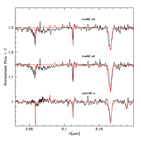
Figure 21: Best CMFGEN fits (red) of RCW 82 and RCW 120 ionizing sources spectra (black).

Figure 22: Normalized SINFONI YSO spectra. Panel a, b, c and d show respectively the Br$\gamma$, H₂, CO emission and CO absorption dominated spectra.

Figure 23: Spectra of YSOs with composite features.

Appendix B Notes on individual objects

Here, we briefly summarize the main characteristics of each region. Figs. 24 to 30 provide source identification as well as linemaps of a few YSOs.

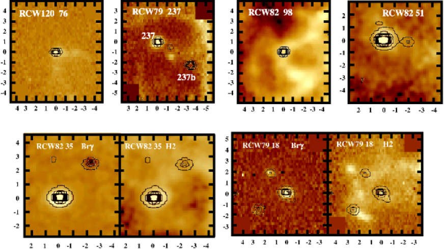
Figure 24: Top panels: H₂ maps of YSOs with contours of the full K-band images overplotted. The H₂ emission is more extended than the bulk of the K-band emission. Bottom panels: Br$\gamma$ and H₂ maps of RCW82 35 and RCW79 18 together with contours of the full K-band emission. In all panels, North is up and East is to the left. The axis indicates the RA and DEC offsets (in arcseconds) relative to the main YSO (see Table LABEL:tab_yso for coordinates).

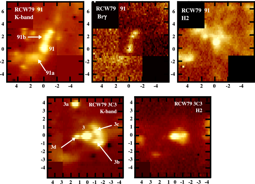
Figure 25: Identification of the sub-components of YSOs RCW79 91 (top panels) and RCW79 3C3 (bottom panels) together with Br$\gamma$ and H₂ maps. North is up and East is to the left. The axis indicates the RA and DEC offsets (in arcseconds) relative to the main YSO (see Table LABEL:tab_yso for coordinates).

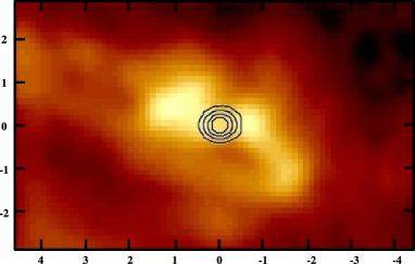
Figure 26: Morphology of RCW79 2C3. The image shows the H₂ emission (created from the initial datacubes smoothed with a spatial Gaussian – FWHM = 3 pixels). North is up, East is to the left. The axis indicate the offsets (in arscseconds) relative to the YSO position (coordinates given in Table LABEL:tab_yso).

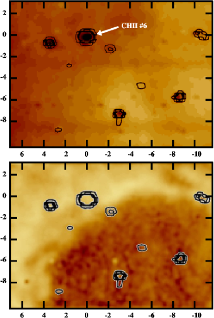
Figure 27: Br$\gamma$ (top) and H₂ maps of the the compact H ii region on the border of RCW 79. The contours of the full K-band emission are shown in black. North is up and East is to the left. The axis indicates the RA and DEC offsets (in arcseconds) relative to source CHII #6.

B.1 RCW 79

Eight sources were observed in this region. All present spectroscopic features typical of YSOs. Sources 237, 91 and 3C3 are resolved in multiple components (respectively Figs. 24 and 25) .

Sources 237-b and 1C4 show a decreasing continuum together with Na i, Ca i and CO absorptions. Source 1C4 also shows Br$\gamma$ in absorption.

Sources 2C3, 3C3 and 237 are dominated by H₂ emission. According to their GLIMPSE colors, they are Class I sources, 3C3 and 237 being the reddest (high $[3.6]-[4.5]$ color). This agrees with 3C3 and 237 having a rising continuum whereas 2C3 has a flat one. Fig. 26 shows the H₂ emission of RCW79 2C3. While the $K$–band features a point source, a more elongated structure is seen in the H₂ map. The emission peak in the latter does not coincide with the YSO in the $K$–band: a large amount of molecular material is still present around the YSO. We could not construct the H₂ velocity map due to the weakness of the signal in the emitting regions. The H₂ emission does not come directly from the YSO, and this should be kept in mind when interpreting the mixed results of Sect. 5.3 regarding the nature of the emission.

The spectrum of 237 is very similar to the one of source nr56c (Martín-Hernández et al. 2008). A bright $H_{2}$ emission filament is observed in the field of source #237 (Fig. 24). Its velocity is that of the H ii region, and this $H2$ emission filament corresponds to the 8 $\mu$m emission that originates from the nearby PDR.

Sources 18 (Fig. 24), 91 (Fig. 25), 186 and 4C4 show wide Br$\gamma$ emission. A maser was identified by Caswell (2004) in the region around source 91, but its association with any of the near-IR sources is not obvious (see ZA06). Sources 91, 18 and 4C4 are Class I sources, having similar colors in the GLIMPSE color-color diagram.

The field of the compact H ii region shows stellar sources and extended Br$\gamma$ and H₂ emission (Fig. 27). The Br$\gamma$ emission (ionized gas) is confined within a region bounded by a H₂ filament. OB stars are observed as dark spots in the Br$\gamma$ map. Surprisingly, the two brightest ionizing stars of the compact H ii region lie in the direction of the H₂ filament and not in the ionized cavity; this might be a projection effect. The extended Br$\gamma$ emission and H₂ filament have similar velocities, also similar to that of the large central RCW 79 region.

Extended Br$\gamma$ and H₂ emission are observed in the field of source 1C4 (not shown). The Br$\gamma$ emission is probably that of the ionized gas in RCW 79. The H₂ emission comes from the PDR. Both emission indicate velocities similar to that of the central H ii region.

Source 4C4 is a tight cluster composed of one bright objects and 6 much fainter components. They present an increasing spectrum and a faint Br$\gamma$ emission line. No extended emission is observed in this field.

B.2 RCW 82

Five candidates YSOs were observed in the direction of RCW 82, all situated on the border of this H ii region, except possibly 51. Sources 4, 7, 35, and 51 have been classified as Class I by PO09. Source 98 has not been classified, due to uncertain $J$ and $H$ measurements and to an absence of 8 $\mu$m measurement.

Source 4 is almost featureless, with a faint and wide Br$\gamma$ line, and a rising spectrum. This agrees with a Class I source. A fainter source is present in the field, situated south-west of 4; it shows no features, except an increasing continuum.

Source 7 has a rising spectrum with numerous $H_{2}$ lines and CO headbands in emission. A disk is probably present. An $H_{2}$ jet is observed (Fig. 15), confirming the youth of this object. Its evolutionary stage, I or II, is uncertain.

Source 35 shows all types of signatures (Br$\gamma$ and $H_{2}$ lines, CO emission, and an increasing spectrum). Its velocity field is unusual, with Br$\gamma$ emission at the velocity of the H ii region, but strongly approaching $H_{2}$ material. This source has probably a dominant disk and thus is probably a Class II object; ejection is possibly present, but needs confirmation. An extended $H_{2}$ emission is observed in the field (see Fig. 24), at the velocity of the H ii region. It probably comes from the nearby PDR.

Source 51 shows a strong Br$\gamma$ emission line, an increasing spectrum, and faint $H_{2}$ and CO emission. Its high emission in the 24 $\mu$m band indicates that it is probably a rather massive YSO. It lies at the center of a cluster (Fig. 24): several faint continuum sources are present in the field (see also Fig. 17 in PO09).

Source 98 (Fig. 24) shows faint CO features in absorption; however it is most probably a young source (and not an evolved star) as it presents an increasing spectra. A bright extended $H_{2}$ emission is present over the whole field (Fig. A.8), at the velocity of the H ii region. Most probably it is emitted in the vicinity of the PDR as confirmed by the line ratios indicative of a non-thermal process ($\frac{I_{1-0s(1)}}{I_{2-1S(1)}}\sim$ 3.5 and $\frac{I_{1-0s(1)}}{I_{3-2S(3)}}\sim$ 10).

B.3 RCW 120

Ten sources were observed in the direction of RCW 120. Eight of them present spectroscopic features characteristic of YSOs. Two of them are different. They are:

$\bullet$ RCW120 39 was classified as a Class II in DE09. The SINFONI spectrum shows that it is most probably an evolved star, as it presents strong CO absorption features and no other signature typical of YSOs.

$\bullet$ RCW120 C4–64 was also classified as an intermediate Class  I/II source in DE09. However its spectrum is slowly decreasing; there is no Br$\gamma$ nor H₂ emission lines; only the CO bands are observed in absorption. Thus it is probably also an evolved star, located by chance on the border of the C4 condensation.

Note that RCW 120 lies only $\sim$12° of the Galactic center, and thus evolved stars of the Galactic bulge may be present in the background.

RCW120 76 (Fig. 24), 106 and 107 are rather similar, almost featureless, with no or faint Br$\gamma$ line, no or faint H₂ lines and no CO emission bands, along with an increasing continuum. They are possibly the less evolved of the YSOs surrounding RCW 120, mostly dominated by their envelope. They were classified as respectively Class I-II, Class I, and Class I-II in DE09, in good agreement with the present results.

RCW120 49 and 103 are similar, with strong Br$\gamma$ emission, numerous H₂ lines and CO bands, superimposed on an increasing continuum. They are possibly more evolved than the preceding group, the presence of strong CO emission bands pointing to a dominant disk. They were classified as Class I-II and Class I in DE09.

Fig. 28 shows the H₂ emission and velocity maps of RCW120 49. The H₂ emission shows multiple peaks none of which is located at the $K$–band position of the YSO. The H₂ velocity map reveals that the two H₂ peaks on each side of the YSO have different radial velocities. We note however that the H₂ material at velocities of about -80 km s^-1 corresponds to a weak emission region (it is slightly offset compared to the emission peak seen in the H₂ map). The H₂ profile at this position is also peculiar in the sense that it probably results from multiple components, being rather broad and featuring a “shoulder” on the blue side of the main emission peak. On the other hand, the bright emission peak south-east of the YSO is significantly detected at a lower velocity than the YSO itself and do not show any peculiar line profile. The analysis of the H₂ emission lines in Sect. 5.3 indicated thermal emission with a possible small contribution from non thermal emission . The presence of a jet would explain both this emission and the velocity map.

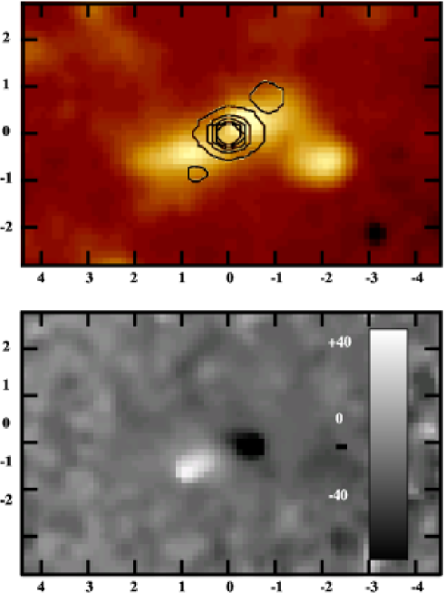
Figure 28: Morphology and dynamics of RCW120 49. Top: H₂ emission map with contours of the full K–band emission overplotted. Bottom: H₂ velocity map (scale is in km s^-1). North is up, East is to the left. The axis indicate the offsets (in arscseconds) relative to the YSO position (coordinates given in Table LABEL:tab_yso).

We have seen previously that YSO RCW120 103 had peculiar kinematical properties, with H₂ moving much faster than Br$\gamma$ (Sect. 5.4). Fig. 29 shed more light on this problem. The H₂ emission peaks at the same position as the $K$–band emission. But an arc/spiral is detected south of the YSO, showing that molecular gas is present on wide scales. The velocity map confirms that a minimum (around -90 km s^-1) is located on the YSO. But this map tend to show that a velocity gradient exists on a direction south-east/north-west across the position of the YSO. A similar map in Br$\gamma$ did not reveal any structure. We note however that the velocity difference between both sides of the H₂ structure is of the order of 20 km s^-1, just at the limit of the resolution of our velocity measurements. Hence, we refrain from interpreting too much this possible structure and simply conclude that the geometry and dynamics of RCW120 103 is probably rather complex. This is confirmed by the velocity of the extended H₂ emission south of the YSO, which is intermediate between the velocity of the H ii region and that of the YSO. We also note that RCW82 35 which showed the same velocity discrepancy as RCW120 103 (H₂ velocity much larger than Br$\gamma$ velocity) did not reveal any velocity structure.

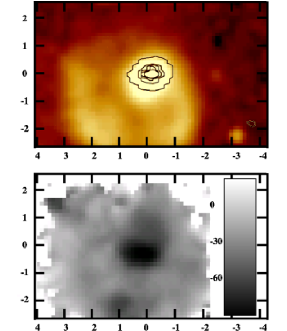
Figure 29: Same as Fig. 28 for YSO RCW120 103.

The field of RCW120 51 contains several sources (Fig. 14), all observed in the direction of the ionized gas. We see on the spectra the Br$\gamma$ emission of the ionized gas. The three brightest sources have a decreasing continuum; source 51b and 51c present CO absorption bands. These two sources are probably stars and not YSOs. Source 51a is probably an YSO, as its spectrum show Br$\gamma$ emission and no CO absorption. However we do not confirm the Class I classification of DE09. YSO 51a lies at the tip of a “finger”, a structure of the ionization front bright in the mid-IR. The proximity of this structure has probably hampered the photometric measurements of this object.

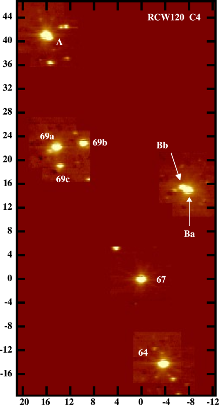
Figure 30: Identification of YSOs in condensation 4 of RCW 120. North is up and East is to the left. The axis indicates the RA and DEC offsets (in arcseconds) relative to source 67.

Condensation 4 contains several sources with different properties (Fig. 30). Sources A and Ba/Bb are respectively at the center of zones of extended 8 $\mu$m and 24 $\mu$m emission resembling small PDRs. The $JHK$ 2MASS photometry of the central objects point to late B stars (DE09). The SINFONI spectra of these 3 sources show decreasing continua. Source A shows both Br$\gamma$ and CO absorption. This might result from the blending of two sources, one with each type of features, or be indicative of a medium type star. Source Ba has Br$\gamma$ in absorption and is most likely a B star, while source Bb features CO absorption bands and is either a late type star or a YSO (see Sect. 5.1). Three sources are observed in the field of RCW120 69. They all have a flat continuum. RCW120 C4-69a is featureless. RCW120 C4-69c has CO absorption bands. RCW120 C4-69b show faint CO absorption bands but Br$\gamma$ in emission. Extended H₂ emission is observed south–east of the main source. These sources are probably evolved YSOs, RCW120 C4-69b being the youngest. RCW120 C4-69, considered as a single source, was classified Class I by DE09. However it is not a Class I, but more probably a Class II or III.