Solid-Liquid Interface Free Energy through Metadynamics simulations

Abstract

The solid-liquid interface free energy $\gamma_{sl}$ is a key parameter controlling nucleation and growth during solidification and other phenomena. There are intrinsic difficulties in obtaining accurate experimental values, and the previous approaches to compute $\gamma_{sl}$ with atomistic simulations are computationally demanding. We propose a new approach, which is to obtain $\gamma_{sl}$ from a free energy map of the phase transition reconstructed by metadynamics. We apply this to the benchmark case of a Lennard-Jones potential and the results confirm the most reliable data obtained previously. We demonstrate several advantages of our new approach: it is simple to implement, robust and free of hysteresis problems, it allows a rigorous and unbiased estimate of the statistical uncertainty and it returns a good estimate of of the thermodynamic limit with system sizes of a just a few hundred atoms. It is therefore attractive for using with more realistic and specific models of interatomic forces.

I Introduction

Many important phenomena occurring in first order phase transformations, such as nucleation and growth, are controlled by interfacial properties. In the theory of solidification, one such property is the solid-liquid interfacial free energy $\gamma_{sl}$. This parameter controls the barrier for nucleation of a solid in an undercooled liquid and the transitions between planar, cellular and dendritic growth regimes in metals, which in turn governs their final microstructure woodruff . Despite its importance for both theoretical models and practical applications, accurate data for the value of $\gamma_{sl}$ are not known even for the case of simple elements. There are indeed few experimental techniques aimed at measuring this quantity (for a comprehensive review see Ref.kelton ) and their application is complicated by the very strict control on all experimental parameters that must be achieved to obtain accurate data. One such method for example involves recovering $\gamma_{sl}$ indirectly from nucleation-rate measurements kelton . In this case, large uncertainties in the measured values arise from the possible occurrence of heterogeneous nucleation from very low-concentration impurities. Reliable theoretical values would therefore be very useful.

Several methods have been developed to calculate $\gamma_{sl}$ from in-silico experiments with molecular dynamics, where complete control of the “experimental” variables is achievable. These methods are the Capillary Fluctuation method (CFM) cfm , different sorts of so-called “cleaving” methods (CM) cleavage_gilmer ; cleavage and a Classical Nucleation Theory (CNT) approach cnt . In CFMs the fluctuation spectrum of the interface height is related to the interfacial stiffness $\gamma_{sl}\left(\theta\right)+\gamma_{sl}^{\prime\prime}\left(\theta\right)$ (where the second derivative is taken with respect to an angle $\theta$ defining the crystallographic orientation of the surface) through which $\gamma_{sl}$ can be recovered by calculating $\gamma_{sl}+\gamma_{sl}^{\prime\prime}$ for different interface orientations and fitting the results to an expansion of $\gamma_{sl}$ in kubic harmonics kubic . In CMs, as the name suggests, bulk solid and liquid phases are separately cleaved and the different phases are joined to form an interface. In this way, $\gamma_{sl}$ is recovered by measuring the work done during the process. Finally, in the CNT approach, crystalline nuclei of different sizes are inserted into a supercooled liquid and some orientational average of $\gamma_{sl}$ is recovered by measuring the radius of the critical nucleus $R^{*}$ and inserting its value in the classical nucleation theory equation relating $R^{*}$ and $\gamma_{sl}$ (see for example Ref. kaschiev , page 46). We refer the interested reader to the literature for details of these calculations. Successful applications of the aforementioned methods have been reported for model systems such as hard spheres cleavage_gilmer ; cleavage ; cfm_hard and Lennard-Jones potentials cfm_lj ; cleavage_lj ; cnt as well as more realistic semiempirical and quantum-mechanical cfm ; becker2 ; cfm_al ; cfm_mg ; cvm_apl based Embedded Atom eam and Stillinger-Weber stillinger potentials.

The CFM and CNT are derived with macroscale approximations and thus require large simulation supercells of about $10^{5}$ atoms to be applicable and give accurate results. Cleavage methods require somewhat smaller supercells ($\approx 10^{3}-10^{4}$ atoms) but are prone to the error introduced if the sequence of simulations is not completely reversible. A dramatic example would be the complete solidification of the liquid while joining it to the solid due to a large relative fluctuation in the position of the interface alfe . The simulation supercell must contain a relatively large area of interface in order to avoid the occurrence of these events. Moreover, to compute $\gamma_{sl}$ accurately and efficiently, one has to use a cleaving potential which mimics accurately the interactions between the system’s particles cleavage_lj . This must be built in an ad hoc way for every system and can become cumbersome when complex many-body interactions have to be taken into account such as for example in ab-initio-based calculations.

These shortcomings become particularly troublesome if one consider that interface free energies are very sensitive to the details of the empirical potential; for instance, different parameterizations of EAM potentials yield values of $\gamma_{sl}$ which vary by as much as 30% comparison_sl . In order to capture the complex bonding and the unusual local environments present at the solid-liquid interface, and to capture accurately the anisotropy of crystalline surface energies, one must consider more sophisticated models, which reproduce more closely the first-principles total energy.

In the present paper, we discuss a novel technique to compute $\gamma_{sl}$ which aims at being robust, efficient and transferable, and which is a promising candidate to extend the scope of interfacial energy calculations to more complex potentials than previously treated. Briefly, our method reconstructs a coarse-grained free energy surface (FES) using metadynamicsmetadyn ; parrinello-eppur . Such a FES maps out the transition from a single phase to the space of configurations where two phases coexist. The minimum difference in Gibbs free energy between these two regions at the solid-liquid equilibrium temperature is an excess free energy $G_{xs}$, which is equivalent to the interface free energy $\gamma_{sl}$ multiplied by the area $A$ of the interface.

The remainder of this paper is organized as follows. In Section II we present the thermodynamic basis and the details of the method. In Section III we describe the computational details of our simulations. In Section IV we show our results for a simple Lennard-Jones system and critically discuss them in comparison with other available methods. We also speculate on the possibility of implementing this approach together with ab-initio molecular dynamics. Finally, we summarize our main results.

II Methodological details

II.1 Thermodynamic basis

We consider a homogeneous solid or liquid system of $N$ atoms, located in a periodically repeated supercell within an infinite system, at a pressure $P$ and temperature $T$. Its Gibbs free energy $G$ can be written as

$$G_{s(l)}(P,T)=\mu_{s(l)}(P,T)N$$ (1)

where $\mu_{s(l)}$ is the chemical potential of atoms in the solid (liquid) phase. At the melting temperature $T_{m}$, the chemical potentials in the two phases are equal

$$\mu_{s}(P,T_{m})=\mu_{l}(P,T_{m})\equiv\mu(P,T_{m})\,.$$

There exists a second state of the same system at the melting temperature, in which solid and liquid phases coexist, separated by macroscopically planar interfaces that are naturally fluctuating on the atomic scale. Since the chemical potential in the solid and liquid bulk phases at $T_{m}$ is identical, one can write the overall Gibbs free energy as

$$G_{s|l}(P,T_{m})=\mu(P,T_{m})N+G_{xs},$$ (2)

where an excess energy term associated with the interface has been introduced. Such a term will be extensive with respect to the area of the interface, and we can write it as the product of the surface area $A$ and an interface free energy $\gamma_{sl}$, i.e. $G_{xs}=A\gamma_{sl}$.

The most direct approach to the computation of $\gamma_{sl}$ is clearly to calculate the free-energy difference between the bulk phases and the configurations in which planar interfaces are present, as described by Eqs. 1 and 2 respectively. We will obtain this free-energy difference by means of metadynamics simulations, as described in the next section.

II.2 Free energy differences from metadynamics

The use of metadynamics for reconstructing free-energy landscapes has been the subject of many papers and we refer the reader to the excellent review by Laio and Gervasio and references therein metadyn_review , while we only briefly sketch the main ideas here. Metadynamics is a simulation technique based on non-equilibrium molecular dynamics, which is designed to reconstruct a coarse-grained free energy surface (FES) in the space of one or more collective variables $\{s_{i}\}$ that describe the state of the system. Metadynamics reconstructs the FES by adding a bias potential in the form of a Gaussian centered at a specific point in the Collective Variable (CV) space each time that point is visited. The mathematical form of the bias potentials is given by

$$V(\mathbf{s}_{0},t)=\int_{0}^{t}we^{-\frac{(\mathbf{s}(t^{\prime})-\mathbf{s}_{0})^{2}}{2\sigma^{2}}}\mathrm{d}t^{\prime}$$ (3)

which in the discrete version needed to implement the algorithm for computations becomes

$$V(\mathbf{s}_{0},t)=\sum_{i=0}^{N}w\tau e^{-\frac{(\mathbf{s}(i\tau)-\mathbf{s}_{0})^{2}}{2\sigma^{2}}}.$$ (4)

Here $\tau$ is the inverse of the frequency of deposition of the Gaussians, and $N=t/\tau$ is the number of Gaussians accumulated up to time $t$ in the simulation. $w$ is the deposition rate of the Gaussian functions and $\sigma$ their width.

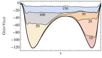
Figure 1: (color online) Schematic representation of the flattening of the effective FES by the repulsive bias of Eq. (4), during a metadynamics simulation in a one-dimensional collective variable space. We show the underlying FES $G(s)$ and the bias accumulated at chosen times (arbitrary units). For a sufficiently long simulation, $G(s)+V(s,t)\rightarrow constant$, so that one can obtain an accurate estimate of the free-energy surface simply by taking the negative of the bias.

The bias discourages the trajectory from remaining indefinitely in the same region of the CV space, effectively pushing the system towards the lowest-lying free-energy barrier. Once all the relevant free energy minima have been levelled by the bias (see Figure 1), the system becomes completely diffusive and wanders freely through all the possible states.

At this stage of the simulation the accumulated bias is equal to the negative of the free energy of the real system plus an additive constant (for a detailed analysis see Ref.metadyn_error1 ). However, there are two limitations in this original form of metadynamics. First of all it is not clear when a metadynamics simulation should be stopped, i.e. when the bias has effectively compensated the underlying free energy. Moreover, even at this point, the effective FES will have a residual roughness of the order of the height of each individual Gaussian ($w\tau$ in equation 4). In order to resolve these issues, the so-called “well-tempered” metadynamics method welltempered_recover has been proposed recently by Barducci et al., and we use this specific type of metadynamics in our simulations. The idea behind well-tempered metadynamics is to gradually reduce the height of the deposited Gaussians, at a rate determined by the magnitude of the bias already present. The expression analogous to (3) reads

$$V(\mathbf{s}_{0},t)=\int_{0}^{t}we^{-\frac{V(\mathbf{s}(t^{\prime}),t^{\prime})}{k\Delta T}}e^{-\frac{(\mathbf{s}(t^{\prime})-\mathbf{s}_{0})^{2}}{2\sigma^{2}}}\mathrm{d}t^{\prime}.$$ (5)

The parameter $\Delta T$ controls how quickly the deposition rate is reduced. Once the simulation approaches convergence, the collective variables space will be sampled with a probability distribution corresponding to an artificial temperature $T+\Delta T$welltempered_orig . Hence, the final bias accumulated during a single simulation converges to

$$V(\mathbf{s}_{0},t)\rightarrow-\frac{\Delta T}{\Delta T+T}G(\mathbf{s}_{0})$$ (6)

The true free energy can be recovered inverting equation (6).

As in any free-energy calculation based on the mapping of the configurations of the system to a coarse-grained collective-variable space, the definition of CVs that can effectively distinguish between relevant states, and describe reliably the natural transformation path is the first, and most important step. The primary requirement is to distinguish the solid phase from the liquid. With this aim, we define for every atom an order parameter $\phi$, which depends on the relative position of its neighbors. The definition of $\phi$

$$\phi(\mathbf{x}_{i})=\frac{\sum_{j\neq i}c_{r}\left(\left|\mathbf{x}_{j}-\mathbf{x}_{i}\right|\right)c_{\alpha}\left(\mathbf{x}_{j}-\mathbf{x}_{i}\right)}{\sum_{j\neq i}c_{r}\left(\left|\mathbf{x}_{j}-\mathbf{x}_{i}\right|\right)}.$$ (7)

contains an angular term $c_{\alpha}$ to distinguish the different environments, and some radial cutoff functions $c_{r}$ which are useful to guarantee that $\phi$ is a continuous function of all its arguments. Note that the weighted sum of $c_{\alpha}$ is normalized over the total coordination, so that $\phi$ is relatively insensitive to fluctuations of the density.

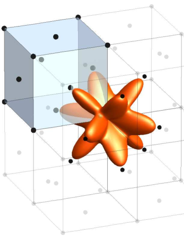
Figure 2: (color online) Angular function $c_{\alpha}(\hat{\mathbf{x}})$ as defined in equation 8. The function is shown as a polar plot, centered on an fcc lattice. $c_{\alpha}$ has well-defined peaks in the directions of the nearest neighbors.

We define the angular function $c_{\alpha}$ as a combination of polynomials in Cartesian coordinates, symmetry adapted to the cubic point group:

$$\begin{split}c_{\alpha}(\mathbf{x})=&\left[x^{4}y^{4}\left(1-z^{4}/\left|\mathbf{x}\right|^{4}\right)+y^{4}z^{4}\left(1-x^{4}/\left|\mathbf{x}\right|^{4}\right)\right.\\ &\left.+z^{4}x^{4}\left(1-y^{4}/\left|\mathbf{x}\right|^{4}\right)\right]\frac{1}{\left|\mathbf{x}\right|^{8}}\end{split}$$ (8)

We have chosen Eq. (8) rather than more traditional parameters such as the so-called $Q_{6}$ (see e.g. q61 ; q62 ; q63 ), for a number of reasons: $c_{\alpha}$ has well-defined peaks for an fcc environment (see Figure 2), it is not rotationally invariant (and will therefore enforce an orientation of the crystal consistent with the periodic boundaries) and it is relatively cheap to compute. It would possible to construct a different form of $c_{\alpha}$ if one wanted to deal with a different crystal structure, and one simply has to rotate the function in order to specify a different crystallographic orientation of the surface. The application of a specialised, orientation-dependent order parameter is a key ingredient of our approach.

The radial cutoff is defined as

$$c_{r}(r)=\begin{cases}1&\quad r\leq r_{1}\\ 0&\quad r\geq r_{0}\\ \left[\left(y-1\right)^{2}\left(1+2y\right)\right]&r_{1}<r<r_{0}\\ \end{cases}$$ (9)

where $y=(r-r_{1})/(r_{0}-r_{1})$. The polynomial part in Eq. (9) is simply a third order polynomial satisfying the constraints of continuity of $c_{r}(r)$ and its first derivative at $r_{1}$ and $r_{0}$.
In order to study the formation of a solid-liquid interface, one must then distinguish configurations where the supercell is completely solid, completely liquid, or partially solid and partially liquid: in the latter case, at least two parallel interfaces will be present. For this purpose we divide the supercell, centered at the origin, into two regions: we assign to region A those atoms having $|z|<\bar{z}$, and to region B all the others (see Figure 3). Note that we take $\bar{z}$ to be about one fourth of the supercell length along $z$, and we keep it constant irrespective of the fluctuations of the supercell’s size. This choice is not troublesome as long as the averages are properly normalized, so that the value of the CVs is independent of the number of atoms contained in each of the regions.

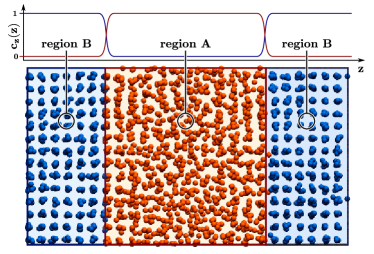
Figure 3: (color online) Cutoff function used to define the regions A and B for the calculation of the two collective variables. The function varies smoothly from 0 to 1 so as to avoid discontinuities when atoms transit between the two regions.

Again, in order to obtain smoothly-varying CVs, we introduce a weight function. We use the same functional form introduced for the radial cutoff; namely, $c_{z}(\mathbf{x})=c_{r}(|z|)$, setting $r_{1}=\bar{z}$, $r_{0}=\bar{z}+\Delta z$ in Eq. (9).

We finally define our CVs $s_{A}$ and $s_{B}$ by averaging the order parameters of the atoms located within region $A$ and $B$, respectively:

$$\begin{split}s_{A}=&\sum_{i}\bar{\phi}(\mathbf{x}_{i})c_{z}(\mathbf{x}_{i})/\sum_{i}c_{z}(\mathbf{x}_{i})\\ s_{B}=&\sum_{i}\bar{\phi}(\mathbf{x}_{i})\left[1-c_{z}(\mathbf{x}_{i})\right]/\sum_{i}\left[1-c_{z}(\mathbf{x}_{i})\right]\end{split}$$ (10)

where

$$\bar{\phi}=\frac{2288}{79}\phi-\frac{64}{79}.$$ (11)

This scaling has been chosen so that $\bar{\phi}=0$ in a homogeneous liquid and $\bar{\phi}=1$ in a perfect fcc solid.

III Computational details

In order to evaluate our method, we decided to perform the metadynamics calculations with a truncated Lennard-Jones potential, in the form used by Broughton and Gilmer gilmer . Such a simple potential is inexpensive and thoroughly studied, yet it can capture many of the relevant physical phenomena occurring in real systems. Its solid-liquid transition, an important ingredient of our approach, has been recently studied by Mastny and de Pablo pablo through a modified Wang-Landau sampling technique landau . Therefore, this system is ideal for a systematic study with our method, comparing it with other techniques and benchmarking its performance as a function of the parameters of the simulation.

We will use Lennard-Jones units throughout the paper. The zero pressure coexistence temperature for this system has been recently recalculated and we take it to be $T_{m}=0.6185$ cleavage_lj ; becker . Details of the phase diagram can be found in ref.becker . We performed our simulations with a range of supercell sizes from $4\times 4\times 6$ fcc unit cells (384 atoms) to $9\times 9\times 20$ (6480 atoms). The supercells were oriented with fcc $[001]$ cell vectors parallel to the axes, with the longest side parallel to $z$, and were rescaled to a volume consistent with the equilibrium density of the solid at the coexistence temperature. Atomic positions were then equilibrated at $T_{m}$ by performing a short molecular dynamics simulation in the canonical (NVT) ensemble. This procedure was adopted in order to generate the starting configurations for the subsequent metadynamics simulations, which we perform instead in the isothermal-isobaric (NPT) ensemble. The timestep for the integration of the equations of motion, performed with a velocity Verlet algorithm frenkel , was $0.004$. This choice gave negligible drift of the conserved quantity in all our simulations.

In order to perform constant pressure simulations, variable-cell dynamics is implemented using a Langevin-piston barostatpiston and a friction of $\gamma_{B}=2$ ps^-1.

The presence of an interface calls for particular attention when performing constant-pressure simulations. In particular, one has to deal with the change in density that occurs when a portion of the supercell melts, at the same time considering fluctuations in the $xy$-plane. If the $xy$-plane parameters of the supercell are fixed, the fluctuations in the solid will be frustrated; on the other hand, if those parameters are left free to vary, one will witness a spurious shrinking of the dimensions in the $xy$-plane due to surface tension whenever an interface is present. In both cases one can in principle observe a strain-related free energy contribution. However, this problem would disappear in the thermodynamic limit, hence one can just make the choice that is more computationally convenient, and consider the resulting error as another finite-size effect, which can be controlled by comparing the results with different supercell sizes. We decided to let only the $z$ component free to fluctuate. In this way, the change of volume occurring as the fraction of liquid and solid phases changes can be accommodated, and even in case of complete melting the $xy$ dimensions remain commensurate with a strain-free solid, which makes it simpler for the system to freeze again into a defect-free solid.

Temperature control is extremely important in metadynamics simulations, since the increase of the biasing potential creates a continuous supply of energy to the system, which must nevertheless be held close to equilibrium in order to sample the free energy correctly. A strong local thermostat is needed, but at the same time one must avoid overdamping, which drastically reduces the diffusion coefficient and hence the sampling of slow, collective modes. We therefore use a colored-noise thermostat ceriotti ; ceriotti2 ; gle4md fitted to provide efficient sampling over a broad range of frequencies, corresponding to vibrational periods between $0.1$ and $10^{3}$ Lennard-Jones time units.

The metadynamics we used for the different simulations are reported in Table 1. This Table also includes data for a number of tests using a single CV, which we describe later. We performed tests with other choices of these parameters spanning about an order of magnitude and no statistically significant changes were observed in the calculated value of $\gamma_{sl}$. The values reported, however, resulted in the best statistical uncertainty in the final free-energy estimate.The simulations were performed using the DL_POLY code (version 2.18, dlpoly ), patched to perform metadynamics using the PLUMEDplumed cross-platform plugin, which greatly reduces the implementation burden by providing a convenient framework for introducing new collective variables.

	# atoms (cell)	$\tau$	$1+\frac{\Delta T}{T}$	$w\tau$
S1 (2D)	2352 ($7\times 7\times 12$)	4	60	0.115
S2 (1D)	384 ($4\times 4\times 6$)	4	40	0.037
S3 (1D)	512 ($4\times 4\times 8$)	4	40	0.037
S4 (1D)	768 ($4\times 4\times 12$)	4	40	0.037
S5 (1D)	1024 ($4\times 4\times 16$)	4	40	0.037
S6 (1D)	1280 ($4\times 4\times 20$)	4	40	0.037
S7 (1D)	1200 ($5\times 5\times 12$)	4	60	0.058
S8 (1D)	2352 ($7\times 7\times 12$)	4	120	0.115
S9 (1D)	6480 ($9\times 9\times 20$)	4	205	0.191

Table 1: Metadynamics parameters for different simulations (1 and 2 dimensional) and different supercell sizes. $\Delta T$ has been chosen such that $k(\Delta T+T)\approx\gamma_{sl}A$ for every size. An order-of-magnitude estimate of $\gamma_{sl}$ suffices for this purpose. $\tau$ was chosen so as to observe the first solid-liquid transition at about half of the total simulation time, and $\sigma$ was set to $0.03$, which is of the order of the thermal fluctuations of the CVs in an unbiased simulation.

When performing simulations at $T>0K$, thermal fluctuations induce some disorder in the solid and the scaled order parameter $\bar{\phi}$ deviates from the value predicted for the ideal fcc crystal. In figure 4 we report the time-averaged order parameter $\left<\bar{\phi}\right>$ and its fluctuations for a single atom in the bulk phases. At the coexistence temperature, the average for the liquid oscillates around zero, while for the solid $\left<\bar{\phi}\right>\approx 0.83$. We note that even for an individual atom the order parameter can distinguish very clearly between the two phases at the melting temperature.

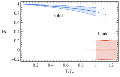
Figure 4: (color online) TIme-averaged value of the order parameter $\bar{\phi}$ for an individual atom in the bulk solid and liquid phases, as evaluated for the LJ system at different temperatures and across the solid-liquid transition. The bounding lines delimit the range one standard deviation above and below the mean value. Dashed lines correspond to the values of the order parameter for metastable solid and liquid. Note that the parameters $r_{1}$ and $r_{0}$ for the radial cutoff (9) are scaled from the values used at $T_{m}$ according to the changes of the equilibrium density.

The parameters entering the radial cutoff function $c_{r}$ have been chosen to be $r_{0}=1.5$ and $r_{1}=1.2$, so as to encompass the typical first-neighbour distances in both Lennard-Jones solid and liquid at $T=T_{m}$. In order to prevent $s_{A}$ and $s_{B}$ from visiting irrelevant configurations, corresponding to an order parameter far from its mean value in either liquid or solid, we have applied a lower and upper wall on both CVs metadyn_review in the form

$$V_{wall}(s)=k\left(\frac{s-s_{limit}}{\epsilon}\right)^{n}$$ (12)

with $k=50$, $\epsilon=0.01$, $n=4$ and $s_{limit}=-0.15$ and $0.95$ for the lower and upper wall respectively, which introduces a restraining potential for $s_{A},s_{B}<-0.15$ and $s_{A},s_{B}>0.9$. At the same time, $V_{wall}$ is set to be zero inside this interval and thus cannot interfere with the dynamics of the system in this region of CV space.

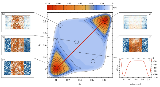
Figure 5: (color online) 2D FES reconstructed by well-tempered metadynamics, together with selected snapshots of configurations obtained during the simulation. Atoms participating in $s_{A}$ are colored in orange, those in $s_{B}$ in blue, and the region of CV space corresponding to each snapshot is marked. The negative peaks in the FES clearly correspond to the two single-phase regions. They are separated by a very wide plateau, corresponding to the presence of well-defined interfaces between solid and liquid phases at various different positions relative to the $A/B$ partition (insets (a), (b), (e)). In inset (f) we report the projection of the FES along the single CV $s=(s_{A}+s_{B})/2$.

IV Results and Discussion

IV.1 Qualitative analysis of the FES

Ideally the FES should be symmetric about the line $s_{A}=s_{B}$. Moreover, as calculations are performed at $T_{m}$, one should observe the occurrence of two minima with the same free energy, at the values of the CVs corresponding to the single bulk phases (either solid or liquid). The expected behavior is clearly exhibited by the calculated FES, reported in Figure 5 for a 7x7x12 supercell, where we show the free-energy landscape together with some snapshots corresponding to different values of the CVs. The combination of CVs $s=(s_{A}+s_{B})/2$ corresponds roughly to the average of $\bar{\phi}$ over the whole box, and distinguishes between configurations with different proportions of solid and liquid phases. It can be used as a convenient reaction coordinate (see Figure 5(f) for the FES projected on $s$). As expected, two wells occur with minima at the complete solid and liquid states, separated by a rather flat region, whose height above the two minima corresponds to the interfacial free energy.

The fact that the two wells should have the same depth can be used to check that the simulation temperature is indeed the melting temperature. This is a significant advantage of our method, since knowledge of the melting temperature is a prerequisite of all the different methods described in the literature to calculate $\gamma_{sl}$. Both the CFM and CM, being based on coexistence simulations, could suffer from major irreversible changes leading to complete solidification/melting of the simulation cell if not performed at the correct temperature, and the data gathered during the simulation would not serve its purpose. Also the CNT method needs the correct value for the melting temperature in order to calculate the nucleation barrier from which $\gamma_{sl}$ is recovered. Our method, by contrast, is still effective even if the simulation temperature is slightly off the actual $T_{m}$. Clearly, an error will be introduced, since $\gamma_{sl}$ is estimated from equation 2 which is satisfied exactly only at $T=T_{m}$. However, our method is very robust, in the sense that it tells us both whether such an error occurs and give us the sign and an estimate of the magnitude of the correction. We will discuss this issue further when addressing finite-size effects.

The two-dimensional FES is rather constant along the line of points equidistant between the two wells, in the direction of the orthogonal combination of CVs $\bar{s}=(s_{A}-s_{B})/2$, since this variable describes the position of the two phases with respect to the partitioning of the cell along $z$ (see snapshots a, b and e in Figure 5). As we will comment further below, our CVs are effective because there exist no metastable phases of the LJ potential correspond to values of the order parameter $\bar{\phi}$ between $\bar{\phi}_{l}$ and $\bar{\phi}_{s}$, and this is likely to be the case for any potentials describing a fcc crystal. Hence, when moving away from the perfect liquid(solid) bulk value, any homogeneous variation of the order parameter would be too energetically costly, and the system instead induces some order(disorder) in the form of small clusters, slowly increasing the free energy (region in orange in Figure 5). Because of the elongated aspect ratio of the supercell, as soon as enough liquid(solid) phase is present, the most favourable configuration corresponds to the presence of two interfaces perpendicular to the $z$ axis. The fact that we observe a solid$\leftrightarrow$liquid transition via the growth of an individual cluster suggests that a very similar approach can be used to study the nucleation process itself. This idea will be explored in future work.

As the time needed by metadynamics to reconstruct the FES is an exponential function of the dimensionality of the coarse grained space, one might wonder if it is possible to speed up calculations by using a single CV. We explored this possibility as follows. Rather than using $s=(s_{A}+s_{B})/2$, we kept a two-dimensional description, but performed metadynamics on $s_{A}$ alone, while atoms in region B are constrained in order to maintain this region of the supercell in a solid state (i.e we apply a restraining lower wall potential which is a function of $s_{B}$, and introduces a penalty in the enthalpy whenever $s_{B}$ deviates too much from $\bar{\phi}_{s}$. The values of the parameters entering in the restraining potential, whose form is described in Section III, are $k=50$, $\epsilon=0.01$, $n=4$ and $s_{limit}=0.7$. This forces region B to remain solid, while region A can sample both solid and liquid phases. In this case, the FES should show a minimum for $s_{A}\approx\bar{\phi}_{s}$ where the supercell is completely in a solid phase and a maximum where $s_{A}\approx\bar{\phi}_{l}$ i.e. when two interfaces are present. Again the difference between these two values is the interface excess energy. Figure 8 (inset (a)) shows the 1D FES reconstructed in this way at different simulation times. The use of a single CV does not have any adverse influence on the calculated value of $\gamma_{sl}$, as we will show in Section IV.2, and the use of this simpler form of metadynamics is fully justified for our purposes.

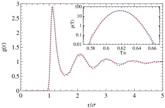
Figure 6: (color online) Radial pair correlation function $g(r)$ for the liquid in the presence of an interface during our metadynamics simulations (red, dashed) and for a normal molecular dynamics simulation of a bulk liquid (blue). It is clear that the two curves are very similar, thus ruling out quantitatively the presence of metastable structures during our simulation. In the inset, the kinetic energy distribution during our simulation is plotted in comparison to that expected for a canonical ensemble at $T=T_{m}$. Again the two are very close demonstrating that the metadynamic bias does not induce any systematic deviation from the correct ensemble, and that quasi-equilibrium conditions hold.

A necessary condition for metadynamics to reconstruct the coarse-grained free energy of the system in a meaningful way is that all the important states and the barriers between them are effectively reached many times during the simulation. Moreover, one has to make sure that quasi-equilibrium conditions hold, which can be monitored by checking temperature and structural relaxation of the system.

In order to check that the system effectively performs many transitions between the single-phase and the two-phase states, we verified that the CVs oscillate several time between their value in the liquid and solid phases. Moreover, we also visually check that the system actually performs these transitions by printing snapshots of the atomic positions and visualising them using the VMD softwarevmd . Quasi-equilibrium conditions hold very accurately, as demonstrated from the inset (b) of Figure 6 where we show the velocity distribution function compared to its analytical equilibrium value. The radial pair correlation function $g(r)$ of the liquid portion of interfacial configurations (Figure 6) agrees well with the one computed for the bulk liquid in an unbiased run, which is a further confirmation that our simulation strategy does not introduce spurious structural effects. The $g(r)$ distribution is a sensitive measure of the short-range order present in the liquid, and any extra structuring would have been clearly detected as a shift of the peak positions or shapes, which does not happen here. The absence of artefacts has also been checked by visual inspection of snapshots of the atomic configurations along the metadynamics trajectory.

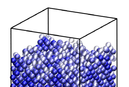
Figure 7: (colour online) A snapshot of the solid-liquid interface taken from the final part of a well-tempered metadynamics simulation. The scaled order parameter $\bar{\phi}$ has been used to colour atoms. The atoms with a liquid-like configuration, with $\bar{\phi}<0.45$ have been hidden, the atoms with $\bar{\phi}>0.65$ have been coloured in blue. Finally, atoms in intermediate configurations, with $0.45<\bar{\phi}<0.65$ have been made translucent. It is clear that - whatever threshold is used to ascertain the solid from the liquid state - the interface is not flat on the atomic scale.

A peculiar feature of our approach is that, at variance with cleavage methods, the solid-liquid interface is created and “annihilated” several times during each simulation, so that hysteresis should be much less of a concern. When the well-tempered bias is nearly converged, the systems diffuse on a flattened FES, and the morphology of the interface corresponds to the most favourable one from a free-energy point of view. As seen from Figure 7, such a morphology includes a significant amount of roughness at the atomic scale. This might be expected from the observation that for the system under consideration the melting temperature is higher than the roughening transition temperature for the $(100)$ surface.

IV.2 Analysis of accuracy and system-size effects

Several terms contribute to the error in calculating a complex thermodynamic property such as $\gamma_{sl}$. In actual applications of this method to a real substance one will be concerned with the accuracy of the total energy and force model, but this is not an issue in our present proof-of-principle case. However, there are still two major sources of error we must be concerned with here; namely, a statistical error stemming from insufficient ergodicity of the sampling (a finite sampling-time error) and the inaccuracies caused from insufficient size of the supercell. These finite-size errors introduce a lower bound on the acoustic vibrational frequencies, and most importantly might affect the structure of the liquid phase, introducing spurious correlation that change the liquid entropy thus changing the melting temperature of the system (although we have seen no evidence for this in the pair correlation function reported above). Moreover, they could in principle induce a strain field in the solid and introduce interactions between the two interfaces.

The finite-sampling error is readily gauged, by performing several independent runs and by checking how quickly the discrepancy between the reconstructed free-energies converges to zero. It is shown in Refs. welltempered_orig ; welltempered_recover that for simple models the error in the FES, after a short transient phase when the free-energy basins are being filled, is expected to decay as the inverse square root of simulation time.

It is reassuring to verify that this behaviour is also found in our system, as shown in Figure 8. This behaviour is to be expected, because for long simulation times well-tempered metadynamics corresponds to a histogram-reweighting with a nearly perfect biasing potential. It means also that rather than running a very long simulation, one can with equal machine efficiency perform several, shorter, independent runs, with great advantages from the point of view of parallelisation.

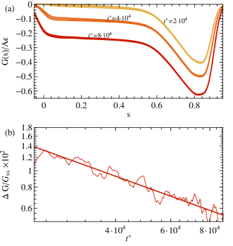
Figure 8: (colour online) Convergence of the FES (inset (a)) and its average error (inset (b)) with respect to time for our 1D simulations. Ten simulations have been performed on a $7\times 7\times 12$ supercell, with the single-CV setup described in the text. The FESs in inset (a) are constructed by averaging equal-times biases of the independent runs, and the error-bars correspond to the standard deviation. In inset (b) we plot such an error, averaged between $\bar{\phi}_{l}$ and $\bar{\phi}_{s}$, as a function of simulation time. The error is plotted on a log-log scale and the least-square linear fit shows that the angular coefficient is close to the theoretical value of $-1/2$ predicted for a simple Langevin model.

In order to calculate the value of $\gamma_{sl}$ from the reconstructed FES, we need to monitor in time the estimate of the excess free-energy due to the interface,

$$G_{xs}(t)=G_{s|l}(t)-G_{s(l)}(t)\rightarrow\gamma_{sl}A\,,$$ (13)

where we label as $G_{s|l}$ the estimate of the free energy for a configuration with a solid-liquid interface. As is routinely done in conventional metadynamics simulations, we take as our best estimate of $G_{xs}$ the incremental average over the final part of the trajectory, well after the initial transient:

$$G_{xs}\approx\frac{1}{t_{f}-t_{i}}\int_{t_{i}}^{t_{f}}G_{xs}(t)\mathrm{d}t\,.$$ (14)

We perform ten independent runs, and we can therefore compute an unbiased estimate of the overall statistical error.

As we previously discussed, in the case of our 2D metadynamics, there are many points on the FES corresponding to coexisting solid and liquid phases, which have the same free energy (see Figure 5); analogously, an extended plateau region is found in the 1D setup. Therefore, any point in these regions would be a valid choice for evaluating the interfacial free energy, provided that these regions are indeed flat. This brings us to the discussion of finite-size errors. In fact, at least for a simple, short-ranged potential such as Lennard-Jones, the greatest concern is the interaction of the two interfaces along $z$, mediated by the elastic strain field in the solid portion and by the altered structure of the liquid in close proximity to the solid/liquid boundary. Such effects are already clearly evident from the 1D FES reported in Figure 9. In the case of very small supercells ($4\times 4\times 6$ and $4\times 4\times 8$ fcc cells, containing 384 and 512 atoms respectively) finite size effects are quite severe and one can hardly see a plateau region. The free energy at these supercell sizes changes quite rapidly over the whole CV space, probably due to the strong interactions between the two interfaces formed during the solid-liquid transition, which are quite close in such short cells. As we increase the length of the supercell at constant $xy$ dimensions, from $4\times 4\times 12$ onwards, another feature of the free energy is observed: one can clearly distinguish a plateau with a linear residual slope. This can be explained by the reduction in the liquid entropy by the constraint of finite $xy$ dimensions of the supercell, which slightly raises the melting temperature. Since the solid is marginally more stable, once the interface is formed there will be a linear increase in free energy as the fraction of liquid phase grows. Indeed, simulations for supercells with larger $xy$ dimensions yield a flatter plateau (see Figure 9(b)). The small increase in melting temperature is expected to manifest itself when the width of the supercell is less than some correlation length $2\leavevmode\nobreak\ L_{corr}$. $L_{corr}$ can be estimated by looking at the distance at which the pair correlation function (see Figure 6) approaches $1$, which in our case is $5\sigma$, corresponding to $\approx 3$ cell parameters, suggesting we need at least $6\times 6$ unit cells in $xy$. Indeed the effect is seen to have vanished by $9\times 9$ unit cells (Figure 9b).

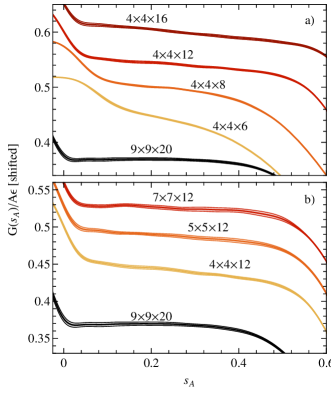
Figure 9: (colour online) (a) The plateau region corresponding to the presence of the solid/liquid interface, with different relative amounts of the two phases, is drawn for different supercell sizes in the $z$ direction. The curves are shifted for display purpose, and they are only meant to demonstrate how the flat portion of $G(s)$ becomes more extended as larger supercells are considered. Finite-size effects are present also in the region for $s<0.1$. In inset (b) we compare results for simulations with different in-plane sizes, showing a further finite-size effect which depends on the change in $T_{m}$ and causes a residual slope of $G(s_{A})/A$ even after the complete formation of an interface.

With these concerns about finite-size effects in mind, we can discuss a reasonable protocol to compute $G_{xs}$. For the 2D metadynamics, the region with $0.35<s_{A},s_{B}<0.55$ is sufficiently flat, and we estimate the free-energy of the two-phases configuration to be $G_{s|l}=G(s_{A}=s_{B}=0.45)$. Let us now consider the 1D case, where region $B$ is restrained to remain solid. In this case, due to the finite slope, the estimate of $\gamma_{sl}$ will depend on which point on the plateau we take to be corresponding to the value of $G_{s|l}$. Hence, we get our best estimate of $G_{s|l}$ as $G(s_{A}=0.2)$ (the point equidistant from the limits of the plateau region) and estimate roughly the systematic error due to the finite slope as $G(s_{A}=0.3)-G(s_{A}=0.1)$.

The results of calculations with different supercell sizes are reported in Table 2, where we report our best estimate of $\gamma_{sl}$ and of the statistical and finite-size errors($\Delta\gamma_{sl}^{stat}$ and $\Delta\gamma_{sl}^{fs}$ respectively). $\Delta\gamma_{sl}^{stat}$ is computed as the root mean square deviation between 10 independent simulations of $10^{7}$ timesteps each. The results of a run using two CVs is also reported for comparison.

	# atoms (cell)	$\gamma_{sl}$ ($\Delta\gamma_{sl}^{stat}$,$\Delta\gamma_{sl}^{fs}$)
S1 (2D)	2352 ($7\times 7\times 12$)	0.37(0.01)
S2 (1D)	384 ($4\times 4\times 6$)	0.39(0.0008,0.02 )
S3 (1D)	512 ($4\times 4\times 8$)	0.390(0.001,0.008)
S4 (1D)	768 ($4\times 4\times 12$)	0.390(0.003,0.005 )
S5 (1D)	1024 ($4\times 4\times 16$)	0.390(0.002,0.006)
S6 (1D)	1280 ($4\times 4\times 20$)	0.390(0.003,0.002)
S7 (1D)	1200 ($5\times 5\times 12$)	0.386(0.003,0.003 )
S8 (1D)	2352 ($7\times 7\times 12$)	0.369(0.002,0.0006)
S9 (1D)	6480 ($9\times 9\times 20$)	0.360(0.003,0.0004)

Table 2: Value of $\gamma_{sl}$ calculated for different supercell sizes with both 1D and 2D metadynamics. The error is reported as $(\Delta\gamma_{sl}^{stat}$,$\Delta\gamma_{sl}^{fs}$), where $\Delta\gamma_{sl}^{stat}$ and $\Delta\gamma_{sl}^{fs}$ are the statistical and systematic error respectively, as defined in the text. For all sets of parameters, ten independent runs have been performed, each $10^{7}$ steps long.

IV.3 Comparison with other methods

With the aid of Table 2 we can now discuss the relative merits of our technique. First of all it can be seen that our calculated value for the (100) surface is very close to the ones calculated by CFM($0.369\pm 0.008$) and CM ($(0.371\pm 0.003)$ in Ref.cleavage_lj and $(0.34\pm 0.02)$ in Ref.cleavage_gilmer ). Although we cannot make such a direct comparison with CNT (because only an averaged value for $\gamma_{sl}$, $\gamma_{sl}^{avg}$ for all possible orientations is given) we point out that their value of $\gamma_{sl}^{avg}=0.302\pm 0.002$ is much lower than ours. The anisotropy in $\gamma_{sl}$ accounts for part of the difference, as the (110) and (111) surfaces have a lower $\gamma_{sl}$ cfm_lj , but we suggest that the anisotropy is too small to account for all of it. The fact that the value calculated by CNT is much lower than both ours and that of the CFM and CM may also be due to the curvature and temperature dependence of $\gamma_{sl}$; CNT is the only method dealing with curved interfaces at temperature below the equilibrium $T_{m}$, as noted in cnt . We also point out here that we do not neglect the $pV$ term as done in the first version of the CM approachcleavage_gilmer , but we still recover a free energy higher than that calculated by CNT. This should rule out the possibility, as supposed in Ref. cnt , that relaxations in volume during the formation of the interface could be another explanation for the discrepancies in $\gamma_{sl}$.

In part, the existence of a small discrepancy between results of CM, CFM and the present work, which rely on similar thermodynamic assumptions, can be explained in terms of differences in the technical details of the calculations. For instance, in some of the CM calculations temperature-control has been implemented by a non-standard velocity-rescaling method, which might affect the accuracy of sampling of the canonical ensemble. In the present work we have tried to highlight all the possible sources of statistical and systematic error, to facilitate further comparison. In any case, the discrepancy between different numerical approaches is negligible when compared to the errors affecting experiments, which can give results differing by as much as 300% (see e.g. Ref dominique ). Hence, any of the aforementioned techniques can be extremely valuable in assisting the interpretation of experimental data and the development of new materials.

The small system size required for our simulations will be a particular advantage, since system size is by far the biggest limitation in applying more sophisticated potentials. We obtain reliable results with system sizes as small as about $1000$ atoms, more than two order of magnitude smaller than required by both CFMs and CNT. CMs require a few thousand atoms, so the advantage is less impressive. However, we remark that the lower bound attainable by CM is most likely set by the need to mitigate hysteresis effects, while with our metadynamics approach this is not an issue, and the limiting factor here will be the kind of interactions between interfaces that are inevitable in all total energy calculations based on periodic boundary conditions.

In view of the large experimental inaccuracies in the measure of $\gamma_{sl}$ (e.g. Ref. dominique ) even simple empirical potentials would already lead to a quantitative improvement of the knowledge of $\gamma_{sl}$. We are applying our method to some of these cases and the results will be published in a future paper. Nevertheless, it may be that the accuracy or information given by a self-consistent electronic structure method is desired for the interfacial free energy calculation, in which case our approach would still be a promising candidate. With high performance computers, simulating a few hundred atoms for several hundred picoseconds is within the reach of present, widely used molecular dynamics methods employing so-called ab initio (electronic density functional) techniques for the calculation of interatomic forces. This would probably result in better predictive power and smaller overall errors despite the possibility of mild finite-size effects.

With a view to performing calculations with more sophisticated potentials, metadynamics offers a further advantage over the other techniques. One could implement a process of iterative refining, whereby one performs a sequential set of calculations with potentials of increasing sophistication and computational cost, in order to reduce the burden of levelling the FES. In fact, the major features of the FES can be captured by the use of very simple potentials reproducing the nearest neighbour bonding in the real material. This first level FES, $G^{(0)}(s)$, could then be used as the initial bias for a second metadynamics run, to be performed with a more accurate (and expensive) potential. At this stage, one will have the much easier task of correcting the discrepancy between $G^{(0)}(s)$ and the FES of the new potential, $G^{(1)}(s)$. This scheme could be repeated with increasingly accurate potentials.

V Conclusions

In the present paper we have presented a novel approach to the calculation of the solid-liquid interface free energy $\gamma_{sl}$, and discussed its application to the calculation of $\gamma_{sl}$ for the $(100)$ surface of a Lennard-Jones solid in contact with its liquid. Our method is based on the definition of a new order parameter, which is designed to identify fcc-ordering of atoms in the orientation of choice, compatible with the periodic boundary conditions, and uses metadynamics simulations to estimate free-energy differences between the bulk phases and configurations where macroscopically flat interfaces are present. We obtain results for $\gamma_{sl}$ in good agreement with previously proposed methods. Moreover, our technique offers several advantages compared to previous approaches discussed in the literature. It requires fewer atoms than those methods based on macroscale approximations, such as measuring capillary fluctuations or the critical nucleation radius, while being less affected by hysteresis than cleavage methods, since the interface is created and destroyed several times during each simulation as equiprobable sampling of the free energy surface is approached. We discuss at length the different sources of error, and how they can be controlled. In particular, we show that our approach is effective even for supercells containing fewer than 1000 atoms, with finite-size errors whose importance can be gauged easily. For this reason, we speculate that it would be possible to perform an ab initio calculation of $\gamma_{sl}$, at the level of electronic density functional theory. To this end, we suggest that an iterative refinement scheme, which starts with a biased free-energy surface computed from a semi-empirical potential, could be a helpful starting point for obtaining converged results within reasonable computational time. We plan to attempt these calculations in the near future, after having further validated our method by comparison with experiments in the case of a simple metal for which we expect empirical potentials to be adequate.

VI Acknowledgments

The authors thank Alessandro Laio for very fruitful discussions about metadynamics and Mark Asta for an early reading of this manuscript and his valuable comments. We would also like to thank Alessandro Barducci, Max Bonomi and Paolo Raiteri for help with PLUMED and advice about the subtleties of metadynamics. Finally, we gratefully acknowledge the COST Action P19 (Multiscale Modeling of Materials) for travel funding that allowed the collaboration between the authors, and EPSRC for support under Grant No. EP/D04619X.

References

- (1) Woodruff, D. ”The Solid-Liquid Interface”; Cambridge University Press: London, 1st ed.; 1973.
- (2) Kelton, K. ”Solid State Physics”; volume 45 Academic Press: Dordrecht, 1st ed.; 1991.
- (3) Hoyt, J. J.; Asta, M.; Karma, A. Phys. Rev. Lett. 2001, 86, 5530–5533.
- (4) Broughton, J. Q.; Gilmer, G. H. The Journal of Chemical Physics 1986, 84, 5759-5768.
- (5) Davidchack, R. L.; Laird, B. B. Phys. Rev. Lett. 2000, 85, 4751–4754.
- (6) Bai, X.-M.; Li, M. J. Chem. Phys. 2006, 124, 124707.
- (7) Altmann, S. L.; Cracknell, A. P. Rev. Mod. Phys. 1965, 37, 19–32.
- (8) Kashchiev, D. Nucleation: Basic Theory with Applications; volume 1 Butterworth Heinemann: Oxford, 1st ed.; 2000.
- (9) Davidchack, R. L.; Morris, J. R.; Laird, B. B. J. Chem. Phys. 2006, 125, 094710.
- (10) Morris, J. R.; Song, X. J. Chem. Phys. 2003, 119, 3920-3925.
- (11) Davidchack, R. L.; Laird, B. B. J. Chem. Phys. 2003, 118, 7651-7657.
- (12) Becker, C. A.; Hoyt, J. J.; Buta, D.; Asta, M. Phys. Rev. E 2007, 75, 061610.
- (13) Morris, J. R. Phys. Rev. B 2002, 66, 144104.
- (14) Sun, D. Y.; Mendelev, M. I.; Becker, C. A.; Kudin, K.; Haxhimali, T.; Asta, M.; Hoyt, J. J.; Karma, A.; Srolovitz, D. J. Phys. Rev. B 2006, 73, 024116.
- (15) Apte, P. A.; Zeng, X. C. Applied Physics Letters 2008, 92, 221903.
- (16) Foiles, S. M.; Baskes, M. I.; Daw, M. S. Phys. Rev. B 1986, 33, 7983–7991.
- (17) Stillinger, F. H.; Weber, T. A. Phys. Rev. B 1985, 31, 5262–5271.
- (18) Alfè, D. Phys. Rev. B 2009, 79, 060101.
- (19) Morris, J. R.; Mendelev, M.; Srolovitz, D. J. Non-Crys. Sol. 2007, 353, 3565 - 3569 Liquid and Amorphous Metals XII - Proceedings of the 12th International Conference on Liquid and Amorphous Metals, 12th International Conference on Liquid and Amorphous Metals.
- (20) Laio, A.; Parrinello, M. Proc. Nat. Ac. Sci. 2002, 99, 12562-12566.
- (21) Parrinello, M. Physical Biology 247.
- (22) Laio, A.; Gervasio, F. L. Rep. Prog. Phys. 2008, 71, 126601 (22pp).
- (23) Bussi, G.; Laio, A.; Parrinello, M. Phys. Rev. Lett. 2006, 96, 090601.
- (24) Bonomi, M.; Barducci, A.; Parrinello, M. J. Comp. Chem. 2009, 30, 1615-1621.
- (25) Barducci, A.; Bussi, G.; Parrinello, M. Phys. Rev. Lett. 2008, 100, 020603.
- (26) Steinhardt, P. J.; Nelson, D. R.; Ronchetti, M. Phys. Rev. B 1983, 28, 784–805.
- (27) ten Wolde, P. R.; Ruiz-Montero, M. J.; Frenkel, D. Phys. Rev. Lett. 1995, 75, 2714–2717.
- (28) Auer, S.; Frenkel, D. Ann. Rev. Phys. Chem. 2004, 55, 333-361.
- (29) Broughton, J. Q.; Gilmer, G. H. J. Chem. Phys. 1983, 79, 5095-5104.
- (30) Mastny, E. A.; de Pablo, J. J. The Journal of Chemical Physics 2005, 122, 124109.
- (31) Wang, F.; Landau, D. P. Phys. Rev. Lett. 2001, 86, 2050–2053.
- (32) Becker, C. A.; Olmsted, D. L.; Asta, M.; Hoyt, J. J.; Foiles, S. M. Phys. Rev. B 2009, 79, 054109.
- (33) Frenkel, D.; Smith, B. Understanding Molecular Simulations; volume 1 of Computational Science Academic Press: San Diego, 2nd ed.; 1996.
- (34) Feller, S. E.; Zhang, Y.; Pastor, R. W.; Brooks, B. R. J. Chem. Phys. 1995, 103, 4613-4621.
- (35) Ceriotti, M.; Bussi, G.; Parrinello, M. Phys. Rev. Lett. 2009, 102, 020601.
- (36) Ceriotti, M.; Bussi, G.; Parrinello, M. J. Chem. Theory Comp. 2010, 6, 1170.
- (37) GLE4MD, http://gle4md.berlios.de/
- (38) Smith, W.; Yong, C.; Rodger, P. Mol. Sim. 2002, 28, 385-471.
- (39) Bonomi, M.; Branduardi, D.; Bussi, G.; Camilloni, C.; Provasi, D.; Raiteri, P.; Donadio, D.; Marinelli, F.; Pietrucci, F.; Broglia, R. A. Comp. Phys. Comm. 2009, .
- (40) Humphrey, W.; Dalke, A.; Schulten, K. J. Mol. Graph. 1996, 14, 33-38.
- (41) Chatain, D.; Metois, J. Surface Science 1993, 291, 1–13.