Soft dynamics in heavy-light mesons

Abstract:

We compute the radial distributions of the scalar, vector and axial charge density in the heavy-light mesons. We present the results obtained for both the lowest lying static heavy-light mesons as well as for their nearest excitations, with $N_{f}=2$ dynamical quarks of Wilson (Clover) type. We used various improvements of the static heavy-quark actions. From these distributions we were able to compute the corresponding charges and their radii $\left<r^{2}\right>$, the results of which are also presented.

1 Introduction

Lattice QCD is the only ab initio method to compute non-perturbative properties of the bound states of quarks and gluons. In this study, we focus on the dynamics of the light degrees of freedom inside a heavy-light meson. In the static limit ($m_{Q}\to\infty$), we can properly define and compute spatial distributions of matter, of the electric charge and of the axial charge. These can then be compared to various quark models which are still the main tool for describing the dynamics of excited states. The spatial distributions which we present here constitute a detailed testing ground for the quark models, for their choice of parameters, as well as for the basic assumptions, and therefore may be a precious means to select among them and/or to improve them.

2 Static heavy-quark propagator

The latticized version of the static heavy-quark effective theory Lagrangian (HQET), in the frame in which the heavy-quark is at rest, reads [3]

$${\cal L}_{\rm HQET}=\sum_{x}h^{\dagger}(x)\left[h(x)-\mathbf{V_{0}(x-\hat{0})}^{\dagger}h(x-\hat{0})\right]+\delta m(g^{2})h^{\dagger}(x)h(x)$$

• The power divergent term $\delta m(g^{2})h^{\dagger}(x)h(x)$ of the discretized HQET is a regularization artifact.

• $V_{0}(x)$ is either the lattice gauge link variable in time direction, or a combination of links in the neighbourhood of the said link. The former gives the Eichten-Hill action; with the latter, depending on the prescription, various actions are obtained, i.e. FAT6, HYP-1, HYP-2, ….

The static heavy-quark propagator is given by

$$S_{h}(\vec{x},0;\vec{y},t)={1+\gamma_{0}\over 2}\delta(\vec{x}-\vec{y})\ \theta(t)\prod_{n=0}^{t-1}V_{0}^{\dagger}(n)$$

. With the Eichten-Hill action, one immediately realizes that the signal of the two point static-light function deteriorates beyond use long before the ground state of the heavy-light meson can be reliably extracted.

FAT6 action was the first proposed to ameriolate the situation. The more recent HYP-1 [4] and HYP-2 [6] actions further reduce the noise to signal ratio (figure 1). In this study, we show that HYP-1/2 can be improved by simply iterating the HYP procedure.

In short, the HYP procedure consists in decorating a given temporal link by the links situated in its neighboring hyper-cube. We refer the reader to the references to HYP-1/2 above and our paper [12] for details. For earlier computations of these distributions see refs. [10].

Choice of the static action

For the spatial distributions we consider, the heavy quark is only a spectator. It stands still at a point in space, while we measure the values of our desired local operators at the light-light vertex as the light quark is pulled away from the fixed center. This leaves us freedom in the choice of static quark action. Judging from figure 1, HYP-2² action (HYP-2 iterated twice) is the best. Henceforth, results presented are obtained using the that heavy quark action.

\psfrag{psfragTitle}{\Huge${\cal E}_{eff}$}\psfrag{psfragTAGA}{\Large\hskip 18.0pt $\mathbf{FAT6}$}\psfrag{psfragTAGB}{\Large\hskip 18.0pt $\mathbf{HYP1^{\phantom{2}}}$}\psfrag{psfragTAGC}{\Large\hskip 18.0pt $\mathbf{HYP1^{2}}$}\psfrag{psfragTAGD}{\Large\hskip 18.0pt $\mathbf{HYP2^{\phantom{2}}}$}\psfrag{psfragTAGE}{\Large\hskip 18.0pt $\mathbf{HYP2^{2}}$}\psfrag{psfragTAGF}{\Large $\mathbf{Eichten\ Hill}$}\includegraphics{Figues/effmassplain.eps}

\psfrag{psfragTitle}{\Huge$\frac{\mathbf{Error}}{\mathbf{Mean}}$}\psfrag{psfragTAGA}{\Large\hskip 18.0pt $\mathbf{FAT6}$}\psfrag{psfragTAGB}{\Large\hskip 18.0pt $\mathbf{HYP1}$}\psfrag{psfragTAGC}{\Large\hskip 18.0pt $\mathbf{HYP1^{2}}$}\psfrag{psfragTAGD}{\Large\hskip 18.0pt $\mathbf{HYP2}$}\psfrag{psfragTAGE}{\Large\hskip 18.0pt $\mathbf{HYP2^{2}}$}\psfrag{psfragTAGF}{\Large $\mathbf{Eichten\ Hill}$}\includegraphics{Figues/meanerror.eps}

Figure 1: Plot on the left shows the effective mass obtained using six heavy-quark actions (light quark at $\kappa=0.1374$, which is somewhat lighter but close to the physical strange quark mass). The right plot shows the (exponential) growth of the statistical error of the two-point function as the time separation between the sources is increased[5]. Notice that the error on the correlation function with HYP-2 heavy-quarks grows in the same way as with the HYP-1² one. Both sink and source are smeared à la Boyle.

Note also that smearing is highly important for the isolation of ground states in both two/three point function calculations. In our study, we adopt the gauge invariant smearing of Boyle[7]. For the parameters used, we refer the reader to our paper[12]. A more detailed study on the effect of smearing will appear in another paper (work in progress).

3 Distributions

To extract the desired distributions we computed the following three point correlation functions:

$$\begin{array}[]{rrrcll}\lx@intercol j^{P}=(1/2)^{-}\mbox{doublet, i.e. ground states\, }J^{P}=[0^{-},1^{-}],e.g.(B,B^{\ast})\hfil\lx@intercol\\[4.30554pt] C^{(3)}_{\Gamma}(-t_{s1},t_{s2};\vec{r})&={\displaystyle\sum_{\vec{x},\vec{y}}}\left<\rule{0.0pt}{12.0pt}\right.&\bar{h}(x)\gamma_{5}q(x)\ \bar{q}(z+\vec{r})&\Gamma&q(z+\vec{r})\ \left(\bar{h}(y)\gamma_{5}q(y)\right)^{\dagger}&\left.\rule{0.0pt}{12.0pt}\right>_{z-{\rm fixed}},\ \mbox{$\Gamma=\mathbbmss{1},\gamma_{0}$}\\ C^{(3)}_{\gamma_{i}\gamma_{5}}(-t_{s1},t_{s2};\vec{r})&={\displaystyle\sum_{\vec{x},\vec{y}}}\left<\rule{0.0pt}{12.0pt}\right.&\bar{h}(x)\gamma_{5}q(x)\ \bar{q}(z+\vec{r})&\gamma_{i}\gamma_{5}&q(z+\vec{r})\ \left(\bar{h}(y)\gamma_{i}q(y)\right)^{\dagger}&\left.\rule{0.0pt}{12.0pt}\right>_{z-{\rm fixed}}\\[4.30554pt] \lx@intercol j^{P}=(1/2)^{+}\mbox{doublet, i.e. first excited states\, }J^{P}=[0^{+},1^{+}],e.g.(B_{0}^{\ast},B_{1})\hfil\lx@intercol\\[4.30554pt] \widetilde{C}^{(3)}_{\Gamma}(-t_{s1},t_{s2};\vec{r})&={\displaystyle\sum_{\vec{x},\vec{y}}}\left<\rule{0.0pt}{12.0pt}\right.&\bar{h}(x)\mathbbmss{1}q(x)\ \bar{q}(z+\vec{r})&\Gamma&q(z+\vec{r})\ \left(\bar{h}(y)\mathbbmss{1}q(y)\right)^{\dagger}&\left.\rule{0.0pt}{12.0pt}\right>_{z-{\rm fixed}},\ \mbox{$\Gamma=\mathbbmss{1},\gamma_{0}$}\\ \widetilde{C}^{(3)}_{\gamma_{i}\gamma_{5}}(-t_{s1},t_{s2};r)&={\displaystyle\sum_{\vec{x},\vec{y}}}\left<\rule{0.0pt}{12.0pt}\right.&\bar{h}(x)\mathbbmss{1}q(x)\ \bar{q}(z+\vec{r})&\gamma_{i}\gamma_{5}&q(z+\vec{r})\ \left(\bar{h}(y)\gamma_{i}\gamma_{5}q(y)\right)^{\dagger}&\left.\rule{0.0pt}{12.0pt}\right>_{z-{\rm fixed}}\end{array}$$

The matrix elements are extracted after dividing $C^{(3)}$ by the appropriate two point functions

$$\begin{array}[]{rclcccccl}R_{\Gamma}(\vec{r})&=&{\displaystyle C_{\Gamma}(-t_{s1},t_{s2};\vec{r})\over\displaystyle\left({\cal Z}^{S}\right)^{2}\times\exp[-{\cal E}\left(t_{s2}-t_{s1}\right)]}&\stackrel{{\scriptstyle|t_{s1}|,t_{s2}\gg 0}}{{\xrightarrow{\hskip 45.5244pt}}}&\langle B|\bar{q}\Gamma q(\vec{r})|B\rangle&\equiv&f_{\mathbbmss{1}}(r),f_{\gamma_{0}}(r)&\mbox{, $\Gamma=\mathbbmss{1},\gamma_{0}$}\\[-12.0pt] &&\lx@intercol\phantom{{\displaystyle C_{\Gamma}(-t_{s1},t_{s2};\vec{r})\over\displaystyle\left({\cal Z}^{S}\right)^{2}\times\exp[-{\cal E}\left(t_{s2}-t_{s1}\right)]}\;\stackrel{{\scriptstyle|t_{s1}|,t_{s2}\gg 0}}{{\xrightarrow{\hskip 45.5244pt}}}\;}\hfil\lx@intercol&\langle B|\bar{q}\Gamma q(\vec{r})|B^{*}\rangle&\equiv&f_{\gamma_{i}\gamma_{5}}(r)&\mbox{, $\Gamma=\gamma_{i}\gamma_{5}$}\\[-10.0pt] \widetilde{R}_{\Gamma}(\vec{r})&=&{\displaystyle\widetilde{C}_{\Gamma}(-t_{s1},t_{s2};\vec{r})\over\displaystyle\left(\widetilde{\cal Z}^{S}\right)^{2}\times\exp[-\widetilde{\cal E}\left(t_{s2}-t_{s1}\right)]}&\stackrel{{\scriptstyle|t_{s1}|,t_{s2}\gg 0}}{{\xrightarrow{\hskip 45.5244pt}}}&\langle B_{0}^{\ast}|\bar{q}\Gamma q(\vec{r})|B_{1}\rangle&\equiv&\widetilde{f}_{\mathbbmss{1}}(r),\widetilde{f}_{\gamma_{0}}(r)&\mbox{, $\Gamma=\mathbbmss{1},\gamma_{0}$}\\[-17.0pt] &&\lx@intercol\phantom{{\displaystyle\widetilde{C}_{\Gamma}(-t_{s1},t_{s2};\vec{r})\over\displaystyle\left(\widetilde{\cal Z}^{S}\right)^{2}\times\exp[-\widetilde{\cal E}\left(t_{s2}-t_{s1}\right)]}\;\stackrel{{\scriptstyle|t_{s1}|,t_{s2}\gg 0}}{{\xrightarrow{\hskip 45.5244pt}}}\;}\hfil\lx@intercol&\langle B_{0}^{\ast}|\bar{q}\Gamma q(\vec{r})|B_{1}\rangle&\equiv&\widetilde{f}_{\gamma_{i}\gamma_{5}}(r)&\mbox{, $\Gamma=\gamma_{i}\gamma_{5}$}\end{array}$$

$f_{\mathbbmss{1}}$, $f_{\gamma_{0}}$, and $f_{\gamma_{i}\gamma_{5}}$ are repectively the matter, electric and axial charge distributions for the $(1/2)^{-}$-states. The tilde symbol is added to distinguish the distributions for the $(1/2)^{+}$- states ($L=1$). The results are presented in figure 2 for the case of the light quark being of the mass close to that of the physical strange quark. The lattice spacing is about $0.1\ {\rm fm}$.

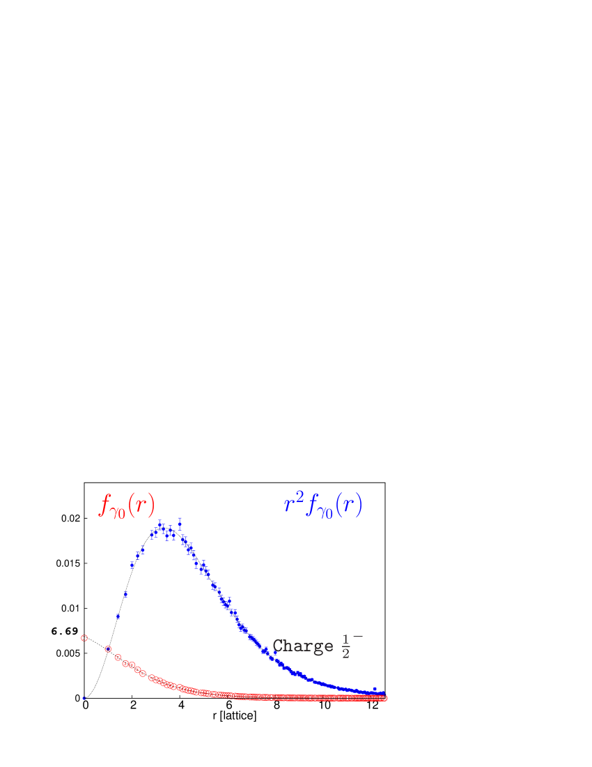
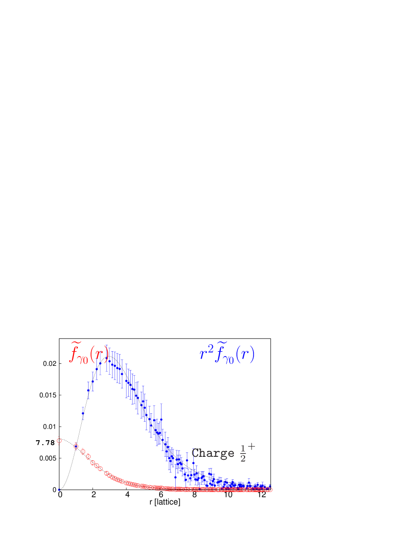
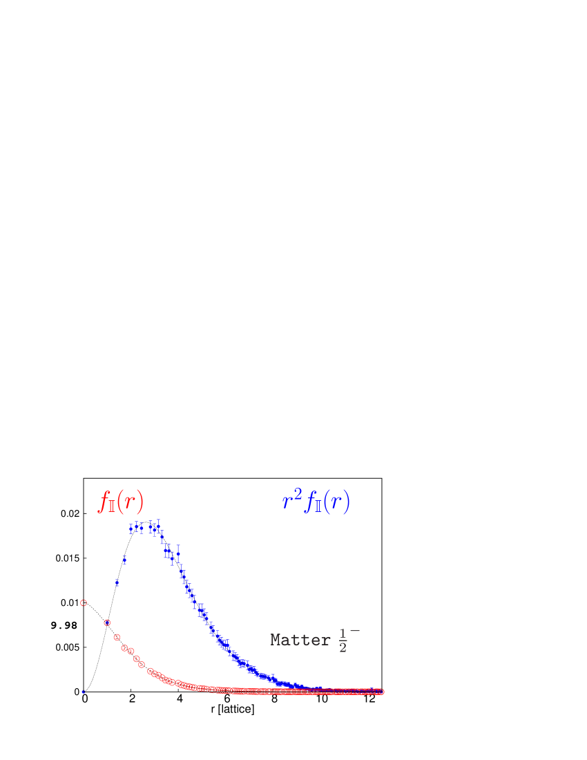
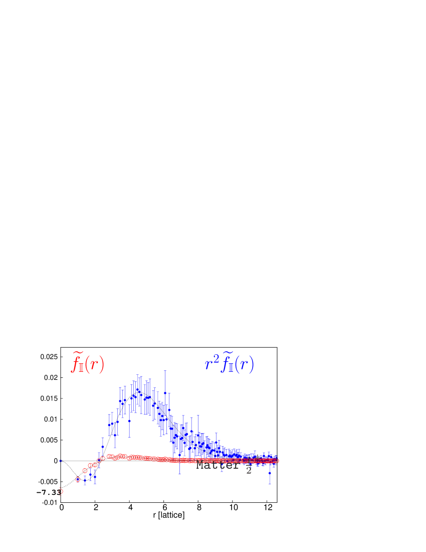
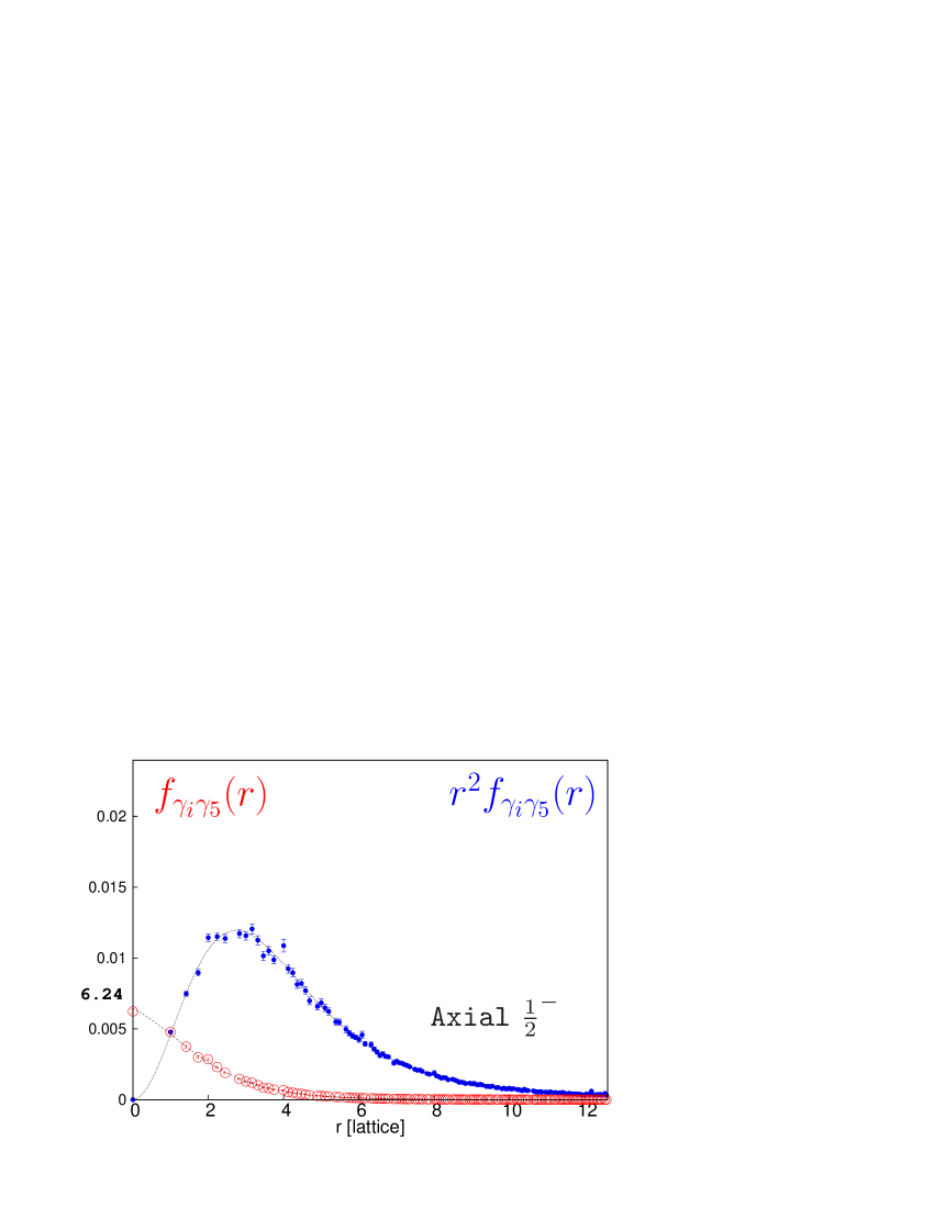
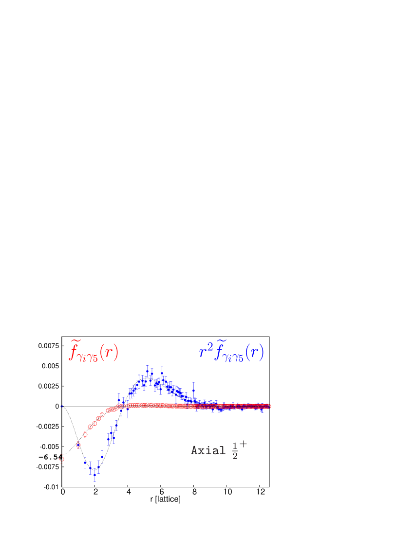
Figure 2: Radial distribution of the vector, axial and the scalar density within the static-light meson. On the left side the distributions are obtained with the external $(1/2)^{-}$ mesons, and those on the right with the $(1/2)^{+}$ ones. light-quark is $\kappa_{q}=0.1374$, which is around the physical strange quark mass. All results are displayed in lattice units.

For more details please see ref. [12]. Here we decide to emphasize the following observations:

• The distributions indeed decrease exponentially when the distance from the static source of color grows. By integrating the distributions over spherical volumes, we see that the cooresponding charges, as a function of radius, already saturate at around $1\ {\rm fm}$.

• We checked that the discrete sum ${\displaystyle\sum_{x,y,z}f_{\Gamma}(x,y,z)}$  and the integral  ${\displaystyle 4\pi\int_{0}^{\infty}f^{fitted}_{\Gamma}(r)\ r^{2}dr}$  are in excellent agreement. This implies that spherical symmetry is well observed. The vanishing of the distribution at the boundaries is a necessary condition.

• Axial and scalar charge distrbutions of the $(1/2)^{+}$-doublet change sign between $0.2$ and $0.4\ {\rm fm}$. The other distributions are monotonically decreasing.

• The vector charge distribution remains of the same form when switching the ground state to the excited ones, which is of course consistent with Ward identity. As for the axial and scalar charge they are completely different (c.f. fig. 2).

4 $\hat{g}$ and $\widetilde{g}$

$g$ and $\widetilde{g}$ are the couplings of the soft pion to the mesons within the same doublet $(1/2)^{-}$ and $(1/2)^{+}$, respectively. Those couplings are related to the emission/absorption of the $P$-wave soft pion, e.g. $B^{\ast}\to B\pi$, and $B_{1}^{\prime}\to B^{0\ast}\pi$. These two axial charges are obtained after integrating the distributions presented in the previous section. In particular, $g$ is given by ${\displaystyle\int_{0}^{\infty}f_{\gamma_{i}\gamma_{5}}(r)\ r^{2}dr}$ (one can use the discrete sum as definition as discussed above.) By using the perturbatively determined matching to continuum, our final values are:

$$\hat{g}=0.526(22)\,,\hskip 54.06023pt\widetilde{g}=-0.157(48)\,,\hskip 54.06023pt\textrm{linear chiral extrapolation}$$ (1)

$$\hat{g}_{\rm HMChPT}=0.444(18)\,,\hskip 22.76219pt\widetilde{g}_{\rm HMChPT}=-0.14(6)\,,\hskip 31.29802pt\textrm{chiral perturbation theory}~{}\cite[cite]{[\@@bibref{}{jernej}{}{}]}$$ (2)

where we indicate the two chiral extrapolation procedures. An important remark is that our result clearly shows that the axial charges $\widetilde{g}\ll\hat{g}$. This is in contradiction with the claims made on the basis of the chiral quark models of refs. [9] that the dynamics within $(1/2)^{-}$ and $(1/2)^{+}$ doublets are very similar [9]. This indeed can be inferred from HMChPT too. However, for that to be the case the charges $g$ and $\widetilde{g}$ should be equal, or at least close to one another, which is clearly not the case.

Notice that $\hat{g}$ reported here is in excellent agreement with the recent results presented in [11] (see also references therein). The pionic transition between the heavy-light mesons belonging to different doublets is more complicated a problem, which will be addressed elsewhere.

5 Charge radius of (Pseudo-)scalar mesons

Electric charge radius is defined by $\sqrt{<r^{2}>}$ where, for the ground state meson,

$$\left<r^{2}\right>_{{\frac{1}{2}}^{-}}=\left.\int_{0}^{\infty}r^{2}f_{\gamma_{0}}(r)\ r^{2}dr\middle/\int_{0}^{\infty}f_{\gamma_{0}}(r)\ r^{2}dr\right.\,,$$

${(\int f_{\gamma_{0}}(r)\ r^{2}dr)^{-1}}$ is simply the Vector Current renormalization constant $Z_{V}$ obtained non-perturbatively. The charge radius for excited state is calculated by substituting $f_{\gamma_{0}}$ by $\widetilde{f}_{\gamma_{0}}$.

In the chiral limit, we obtain $\left<r^{2}\right>_{{\frac{1}{2}}^{-}}=(31.6\pm 0.3)\times a^{2}\;\Longrightarrow\left<r^{2}\right>^{\rm lin.}_{{\frac{1}{2}}^{-}}={\large\mathbf{0.334(3)}}~{}{\rm fm}^{2}$.
For comparison, the vector meson dominance of the electromagnetic form factor

$$\langle B(p^{\prime})|J_{\mu}^{\rm em}|B(p)\rangle=F(q^{2})\left(p+p^{\prime}\right)\,,\quad\left<r^{2}\right>=6\left.{dF(q^{2})\over dq^{2}}\right|_{q^{2}=0}\,,$$ (3)

with $q=p-p^{\prime}$, $J_{\mu}^{\rm em}=e_{Q}\bar{Q}\gamma_{\mu}Q+e_{q}\bar{q}\gamma_{\mu}q$, and $e_{Q(q)}$ being the electric charge of the heavy(light) quark, one obtains that $\left<r^{2}\right>_{\rm VMD}=6/m_{\rho}^{2}={\large\mathbf{0.393}}\ {\rm fm}^{2}$. This result is in good agreement with our result.

References

- [1] A. Ali Khan et al. [CP-PACS Collaboration], Phys. Rev. D 65 (2002) 054505 [Erratum-ibid. D 67 (2003) 059901] [arXiv:hep-lat/0105015].
- [2] M. Albanese et al. [APE Collaboration], Phys. Lett. B 192 (1987) 163.
- [3] E. Eichten and B. R. Hill, Phys. Lett. B 234 (1990) 511.
- [4] A. Hasenfratz and F. Knechtli, Phys. Rev. D 64 (2001) 034504 [arXiv:hep-lat/0103029].
- [5] M. Della Morte et al. [ALPHA Collaboration], Phys. Lett. B 581 (2004) 93 [Erratum-ibid. B 612 (2005) 313] [arXiv:hep-lat/0307021].
- [6] M. Della Morte, A. Shindler and R. Sommer, JHEP 0508 (2005) 051 [arXiv:hep-lat/0506008].
- [7] P. Boyle [UKQCD Collaboration], J. Comput. Phys. 179 (2002) 349 [hep-lat/9903033].
- [8] S. Fajfer and J. F. Kamenik, Phys. Rev. D 74 (2006) 074023 [arXiv:hep-ph/0606278].
- [9] W. A. Bardeen, E. J. Eichten and C. T. Hill, Phys. Rev. D 68 (2003) 054024 [arXiv:hep-ph/0305049]; M. A. Nowak, M. Rho and I. Zahed, Acta Phys. Polon. B 35 (2004) 2377 [arXiv:hep-ph/0307102].
- [10] A. M. Green, J. Koponen, P. Pennanen and C. Michael, Phys. Rev. D 65, 014512 (2001), Eur. Phy. J. C 28, 79-95 (2003)
- [11] D. Becirevic, B. Blossier, E. Chang and B. Haas, Phys. Lett. B 679 (2009) 231 [arXiv:hep-lat/0905.3355].
- [12] D. Becirevic, E. Chang and A. Le Yaouanc, Phys. Rev. D 80 (2009) 034504 [arXiv:hep-lat/0905.3352].