Numerical Results for Spin Glass Ground States on Bethe Lattices: Gaussian Bonds

Abstract

The average ground state energies for spin glasses on Bethe lattices of connectivities $r=3,\ldots,15$ are studied numerically for a Gaussian bond distribution. The Extremal Optimization heuristic is employed which provides high-quality approximations to ground states. The energies obtained from extrapolation to the thermodynamic limit smoothly approach the ground-state energy of the Sherrington-Kirkpatrick model for $r\to\infty$. Consistently for all values of $r$ in this study, finite-size corrections are found to decay approximately with $\sim N^{-4/5}$. The possibility of $\sim N^{-2/3}$ corrections, found previously for Bethe lattices with a bimodal $\pm J$ bond distribution and also for the Sherrington-Kirkpatrick model, are constrained to the additional assumption of very specific higher-order terms. Instance-to-instance fluctuations in the ground state energy appear to be asymmetric up to the limit of the accuracy of our heuristic. The data analysis provides insights into the origin of trivial fluctuations when using continuous bonds and/or sparse networks.

I Introduction

We study the ground state ($T=0$) properties of spin glasses on Bethe lattices with Gaussian bond distribution, which are also considered at low but finite temperatures in Ref. Parisi and Rizzo (2010). In many ways, this study resembles that for the bimodal $\pm J$ bond distribution in Refs. Boettcher (2003a, b). Yet, surprisingly, the behavior for finite-size corrections differ significantly between both distributions.

Bethe lattices are $r$-regular graphs Bollobas (1985), i. e. randomly connected graphs consisting of $N$ vertices, each having a fixed number, $r$, of neighbors Mezard and Parisi (2003). We explore the large-$N$ regime of low-connectivity graphs, $r=3,\ldots,15$, which are of great theoretical interest as finite-connected, mean-field models for low-dimensional lattice spin glasses Mézard et al. (1987); Viana and Bray (1985). A great number of studies have focused on various aspects of this conceptually simple model to hone the complex mathematical techniques required to treat disordered systems Mezard and Parisi (1987); Mézard and Parisi (2001); Mezard and Parisi (2003); Parisi and Tria (2002); de Dominicis and Goldschmidt (1989); Mottishaw (1987); Lai and Goldschmidt (1990) or optimization problems Monasson et al. (1999); Mezard et al. (2002); Franz et al. (2001); Wong and Sherrington (1987); Banavar et al. (1987); Zdeborova and Boettcher (2010).

As before in Refs. Boettcher (2003a, b), we use the Extremal Optimization (EO) heuristic Boettcher and Percus (2000); Boettcher and Percus (2001a); Hartmann and Rieger (2004) to find approximations to spin glass ground states. In previous papers, we have demonstrated the capabilities of EO in determining near-optimal solutions for spin glasses, the coloring problem Boettcher and Percus (2001a); Boettcher and Percus (2004) and the graph partitioning problem Boettcher (1999); Boettcher and Percus (2000); Boettcher and Percus (2001b); Percus et al. (2008); Zdeborova and Boettcher (2010). It is generally harder to find good approximations in complex energy landscapes with a local search heuristic, such as EO, for a problem with continuous weights Bauke and Mertens (2004), but some encouraging results exist Middleton (2004). While our results appear to be sufficiently accurate for the prediction of energy averages for systems up to size $N=2048$, more detailed features, such as their fluctuations over the ensemble of instances (requiring higher moments of the energy), are less reliable for system sizes $N>256$ and larger degree $r$. Hence, for Ising spin glass simulations with EO, discrete $\pm J$ bond weights are usually preferable. Based on the experience with the Sherrington-Kirkpatrick (SK) model, scaling properties of thermodynamic observables are generally believed to be universal, independent of the details of the bond distribution used. There, for instance, finite-size corrections are found to scale approximately with $\sim N^{-2/3}$ Boettcher (2005); Bouchaud et al. (2003); Katzgraber et al. (2005); Palassini (2008); Aspelmeier et al. (2008) (just as for the Bethe lattices with bimodal bonds) and even the average ground-state energy density $\left\langle e_{SK}\right\rangle\approx-0.76317\ldots$ is universal for any symmetric bond distribution Mézard et al. (1987). It would be therefore remarkable to find such distinct scaling behavior between distributions at the level of finite-size corrections, as this investigation suggest. Some previous investigations of Bethe lattices with Gaussian bonds Bouchaud et al. (2003); Liers et al. (2003) have been consistent with $N^{-2/3}$-corrections but were based on smaller sizes and significantly less statistics as in our study here. As a possible resolution, we would have to appeal to ad-hoc assumptions about higher-order corrections. (The distinct effects of discrete versus continuous bonds on defect energies in finite-dimensional lattice spin glasses have been studied numerically in Ref. Hartmann and Young (2001), and also with the renomalization group in Ref. Amoruso et al. (2003).) In turn, the variation of corrections with the details of the bond distribution may provide important clues towards extending replica theory to include finite-size effects.

While the value of this work lies in exploring the range of finite-size scaling on sparse random graphs for spin glasses with differing distributions, it also provides a cautionary note about the analysis of data obtained from such systems. In a sparse system, such as a random graph or a randomly diluted lattice, (trivial) normal fluctuations in geometry or in the bond distribution can obscure the physical essence of the problem at hand. We will argue that in such a system we need to focus attention to the actual “cost” $C$ of disorder in terms of the frustration, instead of the energy $E$ itself. Just consider a simple ferromagnet with fixed bonds $J$ on an ordinary random graph $G_{N,p}$ Bollobas (1985), or alternatively, with continuously distributed bonds $J>0$ on a fixed-degree Bethe lattice of size $N$. In either case, the ground state energy has all bonds satisfied, i. e. no cost in the number of frustrated bonds ($C=0$), and ground state cost fluctuations exhibit a $\delta$-peak, correspondingly. But by the central limit theorem, the absolute sum of all bonds

$$B=\sum_{i=1}^{rN/2}\left|J_{i}\right|$$ (1)

has a normal distribution, inherited by the ground state energy fluctuations via $E=2C-B$. We would claim that the relevant fluctuations at finite $N$ are captured by $C$, not $E$, although the thermodynamic averages $\langle E\rangle$ and $\langle C\rangle$ are completely equivalent, of course. In any case, careful distinction is advisable in an environment of competing finite-size corrections, especially when averaging inherently finite samples in simulations.

The effect of these trivial fluctuations is most pronounced in the study of fluctuations in the ground states of the systems, which have been intensely studied in recent years Bouchaud et al. (2003); Andreanov et al. (2004); Boettcher (2005); Boettcher and Kott (2005); Katzgraber et al. (2005); Aspelmeier et al. (2008); Palassini (2008); Parisi and Rizzo (2008, 2009, arxiv.org:0901.1100, 2010). Our numerical data here shows that those fluctuations in the energy density would predict a seemingly interesting cross-over between non-trivial to trivial scaling between system size and degree. In contrast, the cost density fluctuations would predict a slow drift towards triviality at larger system sizes that is setting in earlier for larger system sizes and might be attributable to a decay in accuracy. As these results are somewhat inconclusive, in a related publication Boettcher we will show that these fluctuations on Bethe lattices with a bimodal distribution of bonds behave, again, similar to those of the SK model.

In the following Sec. II, we introduce first the Bethe lattices we used in the numerical calculations. Then, we address the relation between energies and costs in Sec. III. In Sec. IV, we briefly describe the EO algorithm, which is amply discussed elsewhere Boettcher and Percus (2000); Boettcher and Percus (2001a); Hartmann and Rieger (2004). In Sec. V, we finally present our numerical results. Some conclusions are presented in Sec. VI.

II Spin Glasses on Bethe Lattices

Disordered spin systems on random graphs have been investigated as mean-field models for low-dimensional spin glasses or optimization problems, since variables are long-range connected yet have a small number of neighbors. Particularly simple are Bethe lattices of fixed vertex degree $r=k+1$ Mezard and Parisi (1987); Mézard and Parisi (2001); Mezard and Parisi (2003), which are locally tree-like with vertices imagined as possessing one up-direction and $k$ downward branches. Yet, all $r$ directions are fully equivalent in Bethe lattices, and there is no root vertex or any boundary. In comparison to the otherwise more familiar random graphs studied by Erdös and Rény Bollobas (1985), Bethe lattices at a given $N$ and $r$ avoid fluctuations in the vertex degree and in the total number of bonds.

There are slight variations in the generation of Bethe lattices. For instance, to add a bond one could choose at random two vertices of connectivities $<r$ to link until all vertices are $r$-connected. Instead, we have used the method described in Ref. Bollobas (1985) to generate these graphs. Here, all the terminals on the vertices form a list of $rN$ independent variables. For each added bond, two available terminals are chosen at random to be linked and removed from the list. Furthermore, for algorithmic convenience, we reject graphs which possess self-loops, i. e. bonds that connect two terminals of the same vertex. Multiple bonds between any pair of vertices are allowed; otherwise it is too hard to generate feasible graphs for small $N$, especially at larger $r$. Since $r$ remains finite for $N\to\infty$, the energy and entropy per spin would only be effected to $O(1/N)$ by differences between these choices.

III Sampling Ground States on a sparse Graph

Once a graphical instance is generated, be it a Bethe lattice or any other sparse graph, we assign bonds $J_{i,j}$, here randomly chosen from a Gaussian distribution of zero mean and unit variance, to existing links between neighboring vertices $i$ and $j$. Each vertex $i$ is occupied by an Ising spin variable $x_{i}\in\{-1,+1\}$. The Hamiltonian

$$H=-\sum_{\{bonds\}}J_{i,j}x_{i}x_{j}.$$ (2)

provides the energy of the system. For each instance $I$, the energy $E^{(I)}$ is defined as the difference in the absolute weight of all violated bonds, $C^{(I)}$ (the “cost”), and satisfied bonds, $S^{(I)}$, i. e.

$$E^{(I)}=C^{(I)}-S^{(I)};$$ (3)

the larger the satisfied bond-weight $S^{(I)}$ in the instance, the lower its energy $E^{(I)}$. While $C^{(I)}$ and $S^{(I)}$ vary depending on the spin configuration, for each instance

$$B^{(I)} = C^{(I)}+S^{(I)}$$ (4)

is a constant, with $B^{(I)}$ given by Eq. (1). Hence,

$$E^{(I)}=2C^{(I)}-B^{(I)},$$ (5)

provides a direct relation between cost and energy of each instance. Thus, after averaging over a sample $n_{I}$ of instances $I$ of size $N$ (denoted by $\langle\ldots\rangle_{N}$), we obtain by definition for the averages

$$\left\langle E\right\rangle_{N} = 2\left\langle C\right\rangle_{N}-\left\langle B\right\rangle_{N}$$ (6)

and for the variances:

$$\sigma_{N}^{2}\left(E\right) = 4\sigma_{N}^{2}\left(C\right)+\sigma_{N}^{2}\left(B\right)-4cov_{N}\left(C,B\right).$$ (7)

We observe that for the sparse-graph systems with continuous bond weights under consideration here [similar to the ferromagnetic example in the Introduction, where $\sigma_{N}^{2}\left(B\right)=\sigma_{N}^{2}\left(E\right)\sim N$ and $\sigma_{N}^{2}\left(C\right)=cov_{N}\left(C,B\right)\equiv 0$],

$$\sigma_{N}^{2}\left(C\right) \lesssim cov_{N}\left(C,B\right)\ll\sigma_{N}^{2}\left(B\right),$$ (8)

which we demonstrate in Fig. 1. Note that this condition becomes less satisfied when graphs get denser, i. e. $r$ increases. That trend is indicated by arrows in Fig. 1. The situation described by Eq. (8) does not impact the relation between the averages in Eq. (6) in any way, in particular, not the thermodynamic quantities and their finite-size corrections discussed below. But it does significantly affect both, the error analysis for that data and the interpretation of the ground state energy fluctuations, each derived from the variance. Similarly, $\sigma_{N}^{2}\left(B\right)$ can not be neglected in a fluctuating geometry, such as a random graph or a random-diluted lattice Boettcher (2004a, b), even if the individual bond-weights are sharp, $\left|J_{i,j}\right|\equiv J_{0}$ with constant $J_{0}$.

Eq. (8) does not apply for a discrete bond distribution on a Bethe lattice Boettcher (2003a, b), where $\sigma_{N}^{2}\left(B\right)\equiv 0$; $E$ and $C$ are then equivalent stochastic variables in every respect. Furthermore, in a dense graph such as the SK model Sherrington and Kirkpatrick (1975), and independent of any symmetric bond distribution, this situation is entirely distinct, as even for ground states almost exactly half of all bonds are violated, i. e. $2C^{(I)}\approx B^{(I)}$ for large $N$, and the energy appears merely as an extreme value within the normal fluctuations of $2C$ and $B$. In this case, using $C$ to study fluctuations would be futile. As $r$ is increasing, this trend is already visible in Fig. 1: the gap between the variance in $E$ and $C$ is closing, and is bound to cross over at some larger degree $r$.

Eqs. (7-8) imply that the standard error of the average energy is dominated by the error in $B$,

$$\Delta E_{N} = \frac{\sigma_{N}\left(E\right)}{\sqrt{n_{I}}}\sim\Delta B\left(1-\frac{2cov_{N}\left(C,B\right)}{\sigma_{N}^{2}\left(B\right)}\right),$$ (9)

which by Eq. (8) is larger than that of $C$ for the range of degrees $r$ used in this study. Therefore, our strategy for determining the average ground state energy in the thermodynamic limit will be based on an extrapolation for large $N$ of the values for $\left\langle C\right\rangle_{N}$ and the evaluation of Eq. (6) at $N=\infty$ using the exact value of the bond-density $\left\langle b\right\rangle_{\infty}$, here,

$$\left\langle b\right\rangle_{\infty} =\lim_{N\to\infty}\frac{\left\langle B\right\rangle_{N}}{N}= \frac{r}{2}\left\langle\left|J\right|\right\rangle_{\infty}=\frac{r}{\sqrt{2\pi}}\qquad$$ (10)

for Bethe lattices with a Gaussian bond distribution.

More significantly, when Eq. (8) holds, the variance in the ground state energy fluctuations tracks the variance of $B$, making it apparently trivial (i. e. normal):

$$\sigma_{N}^{2}\left(E\right) \sim \sigma_{N}^{2}\left(B\right)\sim N.$$ (11)

The scaling of $\sigma_{N}\left(E\right)\sim N^{1-\rho}$ has been the focus of keen interest for various mean-field models recently Bouchaud et al. (2003); Andreanov et al. (2004); Boettcher (2005); Boettcher and Kott (2005); Katzgraber et al. (2005); Aspelmeier et al. (2008); Palassini (2008); Parisi and Rizzo (2008, 2009, arxiv.org:0901.1100, 2010). There, non-trivial behavior is typically associated with an exponent that obeys $\rho>\frac{1}{2}$.) We claim that due to Eq. (11) any non-trivial deviation for sparse graphs would have to be found in the cost $C$, if it exists at all.

In the following, we will therefore focus on the cost per spin $c=C/N$. We will study the finite-size corrections of the form

$$\langle c\rangle_{N} =\frac{\langle C\rangle_{N}}{N} \sim a+\frac{b}{N^{\omega}}\left[1+\epsilon(N)\right]$$ (12)

with $a\approx\langle c\rangle_{\infty}$, even taking some higher-order corrections $\epsilon(N)\ll 1$ into account. Additionally, we consider the fluctuations in the ground-state cost density, in particular, the scaling of its deviation with finite size,

$$\sigma_{N}\left(c\right) \sim N^{-\rho}.$$ (13)

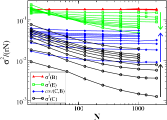
Figure 1: Plot of the variances and co-variances, appropriately rescaled, in Eq. (7) as a function of $N$ for $r=3,4,\ldots,10,15$. (Arrows indicate increasing $r$-values for the adjacent data sets.) All curves are either constant in $N$ throughout, or appear to approach a constant. In this scaling, the variance for the bond weights $B$ (red $\triangle$) collapses for all $r$ to $\sigma^{2}(B)/(rN)=\sigma^{2}\left(\left|J\right|\right)/2=\frac{1}{2}-\frac{1}{\pi}$, and the variances for the energies (green $\square$) are of similar magnitude but declining for larger $r$ (top to bottom). At some fixed (larger) $N$, both, the covariance between $B$ and $C$ (blue $\diamond$) as well as the variance of $C$ (black $\circ$) alone, are quite small, but they are increasing with $r$ (bottom to top).

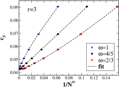
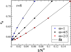
Figure 2: Extrapolation of the average ground state cost per spin for Bethe lattices of degree $r=3,4,\ldots,10,$ and 15 on a $1/N^{\omega}$-scale for $\omega=1$ (${\bf\times}$), $\frac{4}{5}$ (${\bullet}$), and $\frac{2}{3}$ (${\bf\Box}$). The intercept of the fit with the ordinate represents the thermodynamic average (see Tab. 1), which varies weakly with the choice of $\omega$. For each $r$, a fit to the form $a+b/N^{\omega}$, weighted by the error, consistently results in $\omega\approx\frac{4}{5}$ (see Tab. 2 and Figs. 3-4). Only rescaling to $1/N^{\frac{4}{5}}$ virtually linearizes the extrapolation.

IV $\tau$-EO Algorithm for Bethe Lattices

To obtain the numerical results in this paper, we used exactly the same implementation of $\tau$-EO to find ground states as in Ref. Boettcher (2003a), except that we assign to each spin $x_{i}$ in Eq. (2) a “fitness”

$$\lambda_{i}=\left\lfloor 10\frac{x_{i}\sum_{<\dot{,}j>}J_{i,j}x_{j}}{\sum_{<\dot{,}j>}\left|J_{i,j}\right|}\right\rfloor$$ (14)

Instead of using the local field of each variable, which may vary in range somewhat between variables due to the fluctuations in the bond values, we re-scale each variable into the same interval $[-10,-9,-8,\ldots,+10]$, thereby “hashing” the otherwise continuous state-space into a discrete set of up to 21 bins. Note that in this case the sum of the fitnesses is not proportional to the total energy, but good fitness sufficiently correlates with good costs for local search with EO to succeed, as explained in Ref. Boettcher and Percus (2000).

Table 1: Average cost per spin $\left\langle c_{r}\right\rangle_{N}$, plotted also in Fig. 2. The result for $\langle c\rangle_{\infty}$ is based on the value for $a$ in Tab. 2.

$N$	$\left\langle c_{3}\right\rangle_{N}$	$\left\langle c_{4}\right\rangle_{N}$	$\left\langle c_{5}\right\rangle_{N}$	$\left\langle c_{6}\right\rangle_{N}$	$\left\langle c_{7}\right\rangle_{N}$	$\left\langle c_{8}\right\rangle_{N}$	$\left\langle c_{9}\right\rangle_{N}$	$\left\langle c_{10}\right\rangle_{N}$	$\left\langle c_{15}\right\rangle_{N}$
16	0.09043(5)	0.20163(7)	0.3302(1)	0.4703(1)	0.6182(1)	0.7732(2)	0.9326(2)	1.0976(2)	1.9630(3)
32	0.06934(3)	0.16825(5)	0.28476(6)	0.41254(7)	0.54844(8)	0.6908(1)	0.8383(1)	0.9904(1)	1.7954(2)
64	0.05759(2)	0.14934(3)	0.25882(4)	0.37961(4)	0.50894(5)	0.64416(6)	0.78435(6)	0.92878(7)	1.6953(1)
128	0.05087(1)	0.13842(2)	0.24387(2)	0.36103(3)	0.48600(3)	0.61714(4)	0.75324(4)	0.89347(5)	1.63804(6)
256	0.04717(1)	0.13225(1)	0.23544(2)	0.35003(2)	0.47271(2)	0.60153(3)	0.73536(3)	0.87325(3)	1.60540(7)
512	0.04491(1)	0.12853(1)	0.23026(2)	0.34363(2)	0.46465(3)	0.59203(4)	0.72440(4)	0.86153(4)	1.58710(9)
1024	0.04338(4)	0.12616(3)	0.22736(7)	0.33967(8)	0.4601(1)	0.5863(2)	0.7181(2)	0.8545(2)	1.5772(4)
2048	0.04302(2)	0.12577(4)	0.22666(7)	0.3384(1)
$\infty$	0.0420(1)	0.1236(1)	0.2236(1)	0.3352(3)	0.4542(5)	0.5798(8)	0.7103(9)	0.8459(9)	1.561(1)

Table 2: Fit of the data in Tab. 1 to $\langle c_{r}\rangle_{N}=a+\frac{b}{N^{\omega}}$.

$r$	$a$	$b$	$\omega$	ndf	$\chi^{2}$/ndf	$Q$
3	0.041995	0.45	0.81	6	92.5	0
4	0.123592	0.70	0.79	6	58.6	0
5	0.223676	0.97	0.80	5	63.6	0
6	0.335139	1.22	0.80	5	30.3	$6.3\times 10^{-31}$
7	0.454128	1.45	0.79	4	38.2	$5.5\times 10^{-32}$
8	0.579745	1.72	0.79	4	43.6	$1.3\times 10^{-36}$
9	0.710283	1.97	0.79	4	40.4	$6.5\times 10^{-34}$
10	0.845875	2.32	0.80	4	1.8	0.12
15	1.560930	3.65	0.79	4	59.3	0

Table 3: Fit of the data in Tab. 1 to $\langle c_{r}\rangle_{N}=a+\frac{b}{N^{\omega}}+\frac{c\ln N}{N}$.

$r$	$a$	$b$	$\omega$	$c$	ndf	$\chi^{2}$/ndf	$Q$
3	0.041654	0.61	0.78	-0.13	5	37.9	5.5e-39
4	0.123219	0.85	0.77	-0.12	5	50.1	0
5	0.223430	1.06	0.79	-0.07	4	75.8	0
6	0.334402	1.46	0.77	-0.20	4	20.2	1.1e-16
7	0.452726	1.86	0.76	-0.35	3	7.1	8.6e-05
8	0.577866	2.24	0.76	-0.45	3	7.6	4.3e-05
9	0.708515	2.47	0.76	-0.42	3	17.6	2e-11
10	0.845673	2.38	0.80	-0.05	3	2.1	0.1
15		unstable

Table 4: Fit of the data in Tab. 1 to $\langle c_{r}\rangle_{N}=a+\frac{b}{N^{\frac{2}{3}}}+\frac{c\ln N}{N}$.

$r$	$a$	$b$	$c$	ndf	$\chi^{2}$/ndf	$Q$
3	0.042773	-0.21	-0.45	6	2579.1	0
4	0.125082	-0.37	-0.74	6	1792.5	0
5	0.225941	-0.57	-1.07	5	1935.1	0
6	0.337383	-0.60	-1.25	5	1995.7	0
7	0.456151	-0.53	-1.36	4	2392.7	0
8	0.581872	-0.61	-1.59	4	2653.7	0
9	0.713004	-0.76	-1.87	4	2772.5	0
10	0.851120	-1.40	-2.60	4	3212.2	0
11	1.571370	-2.70	-4.58	4	3063.2	0

Table 5: Fit of the data in Tab. 1 to $\langle c_{r}\rangle_{N}=a+\frac{b}{N^{\frac{4}{5}}}+\frac{c\ln N}{N}$.

$r$	$a$	$b$	$c$	ndf	$\chi^{2}$/ndf	$Q$
3	0.041941	0.50	-0.03	6	67.9	0
4	0.123668	0.70	0.01	6	62.9	0
5	0.223727	0.97	0.01	5	64.4	0
6	0.335286	1.21	0.02	5	33.7	1.4e-34
7	0.454604	1.37	0.08	4	57.3	0
8	0.580229	1.66	0.07	4	59.0	0
9	0.710829	1.90	0.09	4	54.6	0
10	0.845843	2.33	-0.01	4	1.7	0.14
11	1.561210	3.44	0.16	4	46.4	4.4e-39

Table 6: Fit of the data in Tab. 1 to $\langle c_{r}\rangle_{N}=a+\frac{b}{N^{\omega}}+\frac{c}{N}$.

$r$	$a$	$b$	$\omega$	$c$	ndf	$\chi^{2}$/ndf	$Q$
3	0.041500	0.12	0.62	0.43	5	35.8	$9\times 10^{-37}$
4	0.123099	0.32	0.68	0.49	5	50.5	0
5	0.223414	0.69	0.75	0.34	4	76.6	0
6	0.334213	0.57	0.69	0.81	4	21.4	$1.2\times 10^{-17}$
7	0.452095	0.52	0.63	1.21	3	7.0	$9.9\times 10^{-5}$
8	0.576847	0.54	0.61	1.54	3	5.6	0.00073
9	0.707617	0.73	0.64	1.61	3	15.0	$9.6\times 10^{-10}$
10	0.845614	2.02	0.78	0.35	3	2.0	0.11
15		unstable

Table 7: Fit of the data in Tab. 1 to $\langle c_{r}\rangle_{N}=a+\frac{b}{N^{\frac{2}{3}}}+\frac{c}{N}$.

$r$	$a$	$b$	$c$	ndf	$\chi^{2}$/ndf	$Q$
3	0.041656	0.16	0.37	6	34.3	$1.2\times 10^{-41}$
4	0.123011	0.29	0.54	6	42.4	0
5	0.222800	0.39	0.74	5	70.5	0
6	0.333995	0.50	0.91	5	17.6	$1.7\times 10^{-17}$
7	0.452686	0.64	1.02	4	7.3	$7.4\times 10^{-6}$
8	0.577985	0.75	1.22	4	8.6	$6.6\times 10^{-7}$
9	0.708256	0.87	1.41	4	12.4	$4.1\times 10^{-10}$
10	0.843511	0.93	1.74	4	17.5	$2.1\times 10^{-14}$
15	1.557000	1.55	2.63	4	146.8	0

To evaluate the proposed $\tau$-EO algorithm, we have benchmarked over a number of exactly solved instances obtained with a branch-and-bound method. Such an approach is clearly limited in attainable system sizes, here $N\leq 64$, and can only be executed for a small test-bed of instances due to the exponential computational cost of exact methods. For larger systems, we have also applied the $\tau$-EO algorithm to a small test-bed of 10 instances of size $N=2^{10}$ for each value of $r$ with 5-times more updates per run and compared results. In the worst case, about 30% of the instances for some $r$ showed a systematic error of about 0.1% or less. Since we sampled over $n_{I}\approx 10^{3}-10^{4}$ instances at this $N$, this systematic error is well below the statistical error of $\sim 1/\sqrt{n_{I}}\gtrsim 1\%$.

Alternatively, we can show that averaged properties obtained with EO are in some sense self-consistent and/or consistent with certain theoretical predictions. For example, Fig. 5 shows the extrapolation for $r\to\infty$ of the already extrapolated thermodynamic ($N\to\infty$) limit of the average energies for each $r$ and $N$. Despite of its derivative nature, the EO data still reproduces the exactly-known ground state energy of SK very accurately.

Finally, it should be kept in mind that settings which provide sufficiently accurate averages of a quantity may be less proficient in determining its higher moments, let alone its entire PDF. Ever higher moments are dominated by rare events (or the lack thereof for finite $n_{I}$) ever deeper in the exponentially suppressed tails of the PDF. For instance, variances are based on (subtractions involving) higher moments and thus can be expected to have substantially boosted systematic errors compared to those quoted for averages.

V Numerical Results

We have simulated Bethe lattices with the algorithm discussed in Sec. IV for $r$ between 3 and 15, and graph sizes $n=2^{l}$ for $l=4,5,6,\ldots,11$ to obtain results for ground state energies. Statistical errors in our averages have been kept small by generating a large number of instances for each $N$ and $r$, typically $n_{I}\approx 10^{6}$ for $N\leq 256$ and $n_{I}\approx 10^{3}-10^{5}$ for $N\geq 512$.

V.1 Average Ground-State Properties

In Tab. 1, we list the values of average costs per spin, $\left\langle c\right\rangle_{N}$. When plotted as a function of $1/N$ in Fig. 2, the average costs per spin for each given $r$ clearly do not extrapolate linearly. Instead, we attempt a fit according to Eq. (12) with variable finite-size correction exponent $\omega$, at first ignoring higher-order corrections ($\epsilon\equiv 0$). Listed in Tab. 2, we find that for the whole range of connectivities $r$ studied here, the fitted scaling corrections appear to be consistent with $\omega=4/5$, and a plot of the data in Fig. 2 on a rescaled abscissa, $1/N^{4/5}$, produces linear scaling. In Fig. 3, we assess the quality of a fit, free of any assumptions about unknown higher-order corrections, by fixing the value of $\omega$ over a range and then fitting for the remaining two parameters, $a$ and $b$, in Eq. (12). Each of the independent data sets for $r=3,\ldots,10,15$ exhibits a strong preference for $\omega\approx 4/5$. In Fig. 4, we plot those fitted values for $\omega$, which within the range of degree values $r$ studied here suggest no trend toward the value of $\omega_{SK}=\frac{2}{3}$ expected for the SK-limit $r\to\infty$, irrespective of bond distribution Bouchaud et al. (2003); Boettcher and Kott (2005); Aspelmeier et al. (2008); Palassini (2008). Plotting the data for $\omega=\frac{2}{3}$ in Fig. 2 clearly does not produce a linear extrapolation as in Refs. Boettcher (2003a, b) for discrete bonds.

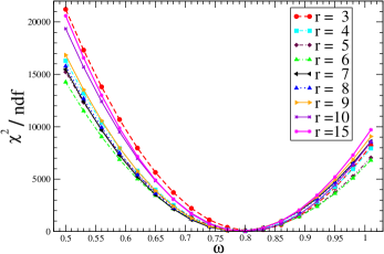
Figure 3: Plot of the $\chi^{2}$ per numbers of degrees of freedom (ndf) for a fit of the data in Tab. 1 to Eq. (12) with only the parameters $a$ and $b$ over a range of fixed $\omega$, ignoring higher-order corrections ($\epsilon\equiv 0$). Independently, for each $r$, the data shows a distinct minimum near $\omega\approx\frac{4}{5}$.

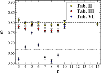
Figure 4: Plot of the fitted values for the finite-size scaling exponent $\omega$ obtained in Tabs. 2 ($\square$) and 6 ($\circ$) for the available values of $r$. Based on an error of $0.01$ estimated from the fits, all values from Tab. 2 are consistent with $\omega=\frac{4}{5}$ (dashed line), without trend for increasing degree $r$ towards $\frac{2}{3}$ (dash-dotted line). The values from Tab. 6 behave less uniformly but seem more centered around $\frac{2}{3}$.

In Tabs. 3-7, we have considered alternative fits to the data involving also higher-order corrections $\epsilon(N)$ to the finite-size corrections, using the full form of Eq. (12). While there are some theoretical results Parisi et al. (1993a, b), obtained for the internal energy near $T_{c}$ in SK, possibly justifying $\omega=\frac{2}{3}$ also below $T_{c}$, little is know to higher order. The expansion for the free energy at $T_{c}$ in Refs. Parisi et al. (1993a, b) provided corrections of the form $c\ln(N)/N$, which could be argued to eventually affect also the ground state energy. We have therefore attempted to fit the data also with higher-order corrections of that form, see Tab. 3, and simply $c/N$, another plausible form. [Unfortunately, a five-parameter fit with a higher-order correction of $c/N^{\alpha}$ does not provide stable results for our data.] Assuming either correction provides the best-quality fit to the remaining four parameters, with the lowest $\chi^{2}$ value relative to the remaining numbers of degree of freedom (ndf), shown in Tabs. 3 and 6. The former fit yields almost identical results to that without higher-order correction, Tab. 2, only that the values for $\omega$ are consistently shifted down by a small amount, see Fig. 4. The fit with $1/N$ drastically changes the fitted values. The values for $\omega$ are now somewhat consistent with $\frac{2}{3}$, but vary widely with degree $r$ in Fig. 4. Fixing $\omega=\frac{2}{3}$ improves the quality of fit (with one less parameter) for $1/N$ corrections to the best fit overall, see Tab. 7. But it becomes entirely inconsistent with $\ln(N)/N$ corrections, as shown in Tab. 4, unlike for fixed $\omega=\frac{4}{5}$ in Tab. 5.

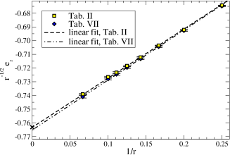
Figure 5: Extrapolated values of the energy densities $\left\langle e_{r}\right\rangle_{\infty}$ obtained from the cost densities $\left\langle c_{r}\right\rangle_{\infty}$ listed in Tab. 1 (yellow $\square$). The data is plotted as a function of inverse degree, $1/r$, and rescaled by a root of the degree, such that the large-$r$ limit approaches the SK model. Similar to the corresponding plot in Ref. Boettcher (2003a, b), the data appears to reach the SK limit virtually on a linear trajectory: a linear fit (dashed line) to all data projects the ground-state of the SK model, $\left\langle e_{SK}\right\rangle=-0.76317$ (marked by $\times$) as $-0.76332$, or to within an error of $<0.1\%$. An extrapolation of corresponding data from Tab. 7 (blue $\diamond$) misses the SK value noticeably (dash-dotted line).

In should be remarked that in all cases, the confidence-of-fit $Q$ is essentially zero in light of the rather tight error bars obtained from the statistics for the average cost densities. We would argue that this is due to the inherent limitations of fitting this data down to small system size $N$ with an asymptotic form valid for large $N$, Eq. (12), as a stand-in for an entirely unknown function of $N$. Hence, these fits should not be dismissed on the basis of $Q$ alone.

The extrapolated values for $a=\left\langle c_{r}\right\rangle_{\infty}$ obtained in Tab. 2 are also listed in Tab. 1. To demonstrate the quality of the extrapolation, we plot in Fig. 5 the derived values for the energy densities by way of Eq. (6), $\left\langle e_{r}\right\rangle_{\infty}=2\left\langle c_{r}\right\rangle_{\infty}-\left\langle b_{r}\right\rangle_{\infty}$, using Eq. (10). As in Refs. Boettcher (2003b, a), already a linear fit to the extrapolated values reproduces the exactly known value of the SK model Mézard et al. (1987); Crisanti and Rizzo (2002); Oppermann et al. (2007) to within an error of $<0.1\%$, confirming to a high degree the numerical accuracy of the data. The obtained slope of the extrapolation, called $f_{1}$ in Ref. Parisi and Tria (2002), which is not expected to be a universal quantity, evaluates to $f_{1}\approx 0.36$, much larger than for the corresponding problem with $\pm J$ bonds Boettcher (2003a, b). The extrapolated costs in Tab. 7, also plotted as energies in Fig. 2, markably miss the SK value.

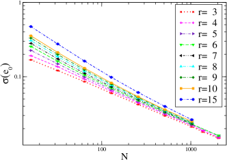
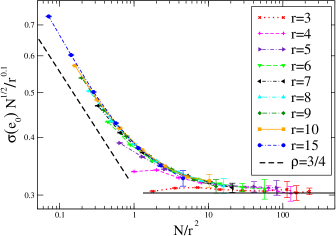
Figure 6: Scaling collapse for the deviation in the ground state fluctuations for the energy densities, $\sigma_{N}(e)$. The raw data for the Bethe lattices is plotted for the available degrees $r$ on top. On the bottom, the same data is plotted, now rescaled by the indicated powers of the degree, with the deviation also multiplied by $\sqrt{N}$, such that trivial, normal fluctuations should plateau (as indicated by the continuous horizontal line). For fixed degree, systematic deviations appear only for sufficiently small $N\lesssim r^{2}$, consistent with a non-trivial scaling $\sigma(e)\sim N^{-\rho}$ at a value of $\rho=\frac{3}{4}$ (dashed line) or even $\rho=\frac{5}{6}$, as expected for the SK model. If taken at face-value, one would conclude that for any fixed degree at large $N$ merely trivial scaling is obtained and only the SK model (or any model with degree growing as $r\gg\sqrt{N}$) has anomalous scaling, $\rho>\frac{1}{2}$.

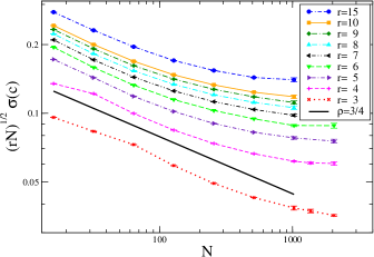
Figure 7: Plot for the deviation in the ground state fluctuations for the cost densities, $\sigma_{N}(c)$. The data for the Bethe lattices is plotted for the available degrees, $r=z$, with the deviation multiplied by $\sqrt{N/r}$, such that trivial, normal fluctuations should plateau. No collapsible scaling regimes emerge, such as a non-trivial scaling $\sigma(e)\sim N^{-\rho}$ with $\rho=\frac{3}{4}$ (continuous line) and much less $\rho=\frac{5}{6}$, as expected for the SK model. Instead, all data appears to steadily approach trivial scaling at much larger system sizes $N$.

V.2 Ground-State Energy and Cost Fluctuations

While the previous section has demonstrated the numerical accuracy of the data at the level of the average of observables, higher moments or a measure of the entire probability density function (PDF) of ground state energy fluctuations provide a more confusing picture. No clear conclusion can be reach on the basis of this data, even when heeding the implications of Sec. III. In light of that discussion, we first present the (as we believe, incorrect) extrapolation for the ground-state energy fluctuations, followed by the corresponding discussion for the cost fluctuations.

In Fig. 6, we show the raw data for the deviations of the energy densities $\sigma_{N}\left(e\right)$ and their apparent collapse. All the data seems to approach trivial, normal fluctuations for sufficiently large system sizes, with a cross-over at ever higher degree $r$. Similar normal fluctuations for this model have been claimed by Ref. Bouchaud et al. (2003). In fact, rescaling the data for a collapse indicates that the cross-over between system size and degree in the Bethe lattice occurs at $N\sim r^{2}$. Taken at face value, this would be a remarkable result. While at any fixed, finite degree a trivial scaling is reached, only in the SK-limit, where system size and degree would scale direct proportionally, $N\sim r$, we would flow towards the left onto the non-trivial branch of the scaling in Fig. 6. Hence, the Bethe lattice results for Gaussian bonds (unlike for $\pm J$ bonds, as we will show in Ref. Boettcher ) are disconnected from the SK-limit. Although this may also explain the unusual finite-size scaling corrections $\omega\approx 0.8$, as well disconnected from the SK-limit, we believe that this data collapse does not probe the true disorder-induced frustration. As we have shown in Sec. III, energy fluctuations are dominated by the variance in the Gaussian distribution of $N$ bonds (although ever less so for larger $r$).

Remarkably, when we plot the deviations $\sigma_{N}\left(c\right)$ for the cost density in Fig. 7, a far more difficult-to-interpret picture results. Unlike for the energy densities in Fig. 6, there is no apparent cross-over but the data instead veers steadily towards normal fluctuations for much larger system sizes. While the data does not show any noticeable statistical errors, it is impossible to exclude a systematic bias in the sampling of ground states with the heuristic, that could manifest itself in a smooth drift away from any potential non-trivial scaling. We can only eliminate the systematic error up to $N\leq 64$ through comparisons with exact ground states obtained with a branch-and-bound algorithm. Above such sizes, we can only argue for small systematic errors based on the internal consistency of the average cost or energies, as is displayed, e. g., in Figs. 2 and 5. Though, this may prove insufficient to guarantee similar fidelity for higher cumulants, like the deviations in the cost. But if we assume sufficient accuracy for this data, it would imply that even for the cost deviations, like for the energies before in Fig. 6, ultimately pure normal fluctuations may result either way when Gaussian bonds are considered. It would not be unusual to find extended transient behavior in spin glasses with Gaussian bonds Boettcher and Cooke (2005).

VI Conclusion

We have found surprising differences in the finite-size scaling behavior between a continuous, Gaussian bond distribution and previous results for a bimodal, $\pm J$ distribution Boettcher (2003a, b) for spin glasses on Bethe lattices of degree $r$. While either distribution leads to equivalent results for thermodynamic averages that smoothly extrapolate to the exactly known SK results with identical scaling in $r$ for $r\to\infty$, the finite-size corrections term $b/N^{\omega}$ not only differ in the correction amplitude $b$ but possibly in the scaling exponent $\omega$ itself. Only when higher-order corrections are postulated, more consistency can be obtained with the value $\omega\approx\frac{2}{3}$ found for discrete bonds on Bethe lattices and for SK with either bond distribution. The value obtained here for Gaussian bonds, $\omega\approx\frac{4}{5}$, raises the question about an eventual cross-over to the SK value at higher $r$. No tendency toward such a cross-over is apparent in our study up to $r=15$. In light of that, the vague expectation of some uncooperative higher-order corrections to $\omega=\frac{2}{3}$ seems preferable, but one might be forgiven to be struck by the solid persistence of $\omega=\frac{4}{5}$ suggested by Figs. 2 and 4.

Our study of fluctuations in the ground-state properties is not successful in determining clearly the scaling behavior of the deviations. But it sends a cautionary note about the origin of fluctuations and the interpretation of data when simulating spin glasses on sparse graphs with continuous bonds or a randomly fluctuating geometry.

References

- Parisi and Rizzo (2010) G. Parisi and T. Rizzo, J. Phys. A 43, 045001 (2010).
- Boettcher (2003a) S. Boettcher, Euro. Phys. J. B 31, 29 (2003a).
- Boettcher (2003b) S. Boettcher, Phys. Rev. B 67, R060403 (2003b).
- Bollobas (1985) B. Bollobas, Random Graphs (Academic Press, London, 1985).
- Mezard and Parisi (2003) M. Mezard and G. Parisi, J. Stat. Phys. 111, 1 (2003).
- Mézard et al. (1987) M. Mézard, G. Parisi, and M. A. Virasoro, Spin glass theory and beyond (World Scientific, Singapore, 1987).
- Viana and Bray (1985) L. Viana and A. J. Bray, J. Phys. C: Solid State Phys. 18, 3037 (1985).
- Mezard and Parisi (1987) M. Mezard and G. Parisi, Europhys. Lett. 3, 1067 (1987).
- Mézard and Parisi (2001) M. Mézard and G. Parisi, Eur. Phys. J. B 20, 217 (2001).
- Parisi and Tria (2002) G. Parisi and F. Tria, Euro. Phys. J. B 30, 533 (2002).
- de Dominicis and Goldschmidt (1989) C. de Dominicis and Y. Y. Goldschmidt, J. Phys. A 22, L775 (1989).
- Mottishaw (1987) P. Mottishaw, Europhys. Lett. 4, 333 (1987).
- Lai and Goldschmidt (1990) P.-Y. Lai and Y. Y. Goldschmidt, J. Phys. A 23, 3329 (1990).
- Monasson et al. (1999) R. Monasson, R. Zecchina, S. Kirkpatrick, B. Selman, and L. Troyansky, Nature 400, 133 (1999).
- Mezard et al. (2002) M. Mezard, G. Parisi, and R. Zecchina, Science 297, 812 (2002).
- Franz et al. (2001) S. Franz, M. Leone, F. Ricci-Tersenghi, and R. Zecchina, Phys. Rev. Lett. 87, 127209 (2001).
- Wong and Sherrington (1987) K. Y. M. Wong and D. Sherrington, J. Phys. A 20, L793 (1987).
- Banavar et al. (1987) J. R. Banavar, D. Sherrington, and N. Sourlas, J. Phys. A 20, L1 (1987).
- Zdeborova and Boettcher (2010) L. Zdeborova and S. Boettcher, J. Stat. Mech. P02020 (2010).
- Boettcher and Percus (2000) S. Boettcher and A. G. Percus, Artificial Intelligence 119, 275 (2000).
- Boettcher and Percus (2001a) S. Boettcher and A. G. Percus, Phys. Rev. Lett. 86, 5211 (2001a).
- Hartmann and Rieger (2004) A. Hartmann and H. Rieger, eds., New Optimization Algorithms in Physics (Wiley-VCH, Berlin, 2004).
- Boettcher and Percus (2004) S. Boettcher and A. G. Percus, Phys. Rev. E 69, 066703 (2004).
- Boettcher (1999) S. Boettcher, J. Phys. A 32, 5201 (1999).
- Boettcher and Percus (2001b) S. Boettcher and A. G. Percus, Phys. Rev. E 64, 026114 (2001b).
- Percus et al. (2008) A. G. Percus, G. Istrate, B. Gonçalves, R. Z. Sumi, and S. Boettcher, J. Math. Phys. 49, 125219 (2008).
- Bauke and Mertens (2004) H. Bauke and S. Mertens, Phys. Rev. E 70, 025102(R) (2004).
- Middleton (2004) A. A. Middleton, Phys. Rev. E 69, 055701(R) (2004).
- Boettcher (2005) S. Boettcher, Eur. Phys. J. B 46, 501 (2005).
- Katzgraber et al. (2005) H. G. Katzgraber, M. Körner, F. Liers, M. Jünger, and A. K. Hartmann, Phys. Rev. B 72, 094421 (2005).
- Palassini (2008) M. Palassini, J. Stat. Mech. P10005 (2008).
- Aspelmeier et al. (2008) T. Aspelmeier, A. Billoire, E. Marinari, and M. A. Moore, J. Phys. A 41, 324008 (2008).
- Bouchaud et al. (2003) J.-P. Bouchaud, F. Krzakala, and O. C. Martin, Phys. Rev. B 68, 224404 (2003).
- Liers et al. (2003) F. Liers, M. Palassini, A. K. Hartmann, and M.Jüenger, Phys. Rev. B 68, 094406 (2003).
- Hartmann and Young (2001) A. K. Hartmann and A. P. Young, Phys. Rev. B 64, 180404(R) (2001).
- Amoruso et al. (2003) C. Amoruso, E. Marinari, O. C. Martin, and A. Pagnani, Phys. Rev. Lett. 91, 87201 (2003).
- Andreanov et al. (2004) A. Andreanov, F. Barbieri, and O. C. Martin, Euro. Phys. J. B 41, 365 (2004).
- Boettcher and Kott (2005) S. Boettcher and T. M. Kott, Phys. Rev. B 72, 212408 (2005).
- Parisi and Rizzo (2008) G. Parisi and T. Rizzo, Phys. Rev. Lett. 101, 117205 (2008).
- Parisi and Rizzo (2009) G. Parisi and T. Rizzo, Phys. Rev. B 79, 134205 (2009).
- Parisi and Rizzo (arxiv.org:0901.1100) G. Parisi and T. Rizzo (arxiv.org:0901.1100).
- (42) S. Boettcher, arXiv:0906.1292 .
- Boettcher (2004a) S. Boettcher, Europhys. Lett. 67, 453 (2004a).
- Boettcher (2004b) S. Boettcher, Euro. Phys. J. B 38, 83 (2004b).
- Sherrington and Kirkpatrick (1975) D. Sherrington and S. Kirkpatrick, Phys. Rev. Lett. 35, 1792 (1975).
- Parisi et al. (1993a) G. Parisi, F. Ritort, and F. Slanina, J. Phys. A 26, 247 (1993a).
- Parisi et al. (1993b) G. Parisi, F. Ritort, and F. Slanina, J. Phys. A 26, 3775 (1993b).
- Crisanti and Rizzo (2002) A. Crisanti and T. Rizzo, Phys. Rev. E 65, 046137 (2002).
- Oppermann et al. (2007) R. Oppermann, M. J. Schmidt, and D. Sherrington, Phys. Rev. Lett. 98, 127201 (2007).
- Boettcher and Cooke (2005) S. Boettcher and S. E. Cooke, Phys. Rev. B 71, 214409 (2005).