Energy Diffusion in Gases

Abstract

In the air surrounding us, how does a particle diffuse? Thanks to Einstein and other pioneers, it has been well known that generally the particle will undergo the Brownian motion, and in the last century this insight has been corroborated by numerous experiments and applications. Another fundamental question is how the energy carried by a particle diffuses. The conventional transport theories assumed the Brownian motion as the underlying energy transporting mechanism, but however, it should be noticed that in fact this assumption has never been tested and verified directly in experiments. Here we show that in clear contrast to the prediction based on the Brownian motion, in equilibrium gases the energy diffuses ballistically instead, spreading in a way analogous to a tsunami wave. This finding suggests a conceptually new perspective for revisiting the existing energy transport theories of gases, and provides a chance to solve some important application problems having challenged these theories for decades.

Diffusive motion is fundamental in nature. The conventional diffusion theory for a particle immersed in a fluid evolves on the basis of the Einstein’s 1905 work on the Brownian motionEinstein (1). It is realized that the motion of the particle can be essentially modeled with the random walksmoluchowski (2), and the corresponding probability distribution function (PDF) is governed by the diffusion equationEinstein (1, 2). This theory predicts the Gaussian PDF, which represents a general class of slower motions in nature. In the last century, it has been verified in a wide range of contexts. For example, the experiments have shown that under normal conditions, i.e., under atmospheric condition and at room temperature, the diffusions of particles are indeed of Gaussian PDF in a variety of systems such as gases, liquids, surfaces of solids, and so on. In fact, the diffusion coefficients of gases provided in manuals of physical propertiesexperience (3), which are useful in the studies of physics, chemistry, meteorology and other sciences, are measured based on the conventional diffusion theory. Due to its great success, such a particle diffusion picture given by the conventional diffusion theory has been the common knowledge in various scientific disciplines.

In a further development of the early transport theory, the clear physical picture of particle diffusion outlined in Einstein’s work was extended by HelfandHelfand (4) in 1960 to link – through a set of generalized Einstein relations – the macroscopic transport coefficients such as those of molecule diffusion, viscosity and thermal transportation on one side, to the corresponding microscopic fluctuating quantities, known as Helfand moments, on the other side, by expressing the former as the linear time increase rates of the statistical variances of the latter. Like the Green-Kubo formulaGreen-1951 (5, 6, 7), Helfand’s theory interprets the transport coefficients in terms of the microscopic dynamics but in a different way, hence provides additional information and insights. In recent years, besides the equivalence between the Green-Kubo formula and the Helfand relations in certain cases, some advantages unique to the Helfand approach have also been realizedViscardy-1 (8, 9).

The Helfand theory addressed the transports of the most important physical quantities including the energy. It is meanwhile the only theory that suggests an answer to the question we focus on in this work, i.e., how the energy initially carried by a particle diffuses. According to the Helfand theory, the energy will diffuse in a random way and the corresponding PDF is Gaussian as well. This could be agreed by most scientists nowadays in view of the overwhelming prevalence of the conventional diffusion theory. However, it should be pointed out that if this is true has never been studied experimentally. Unlike in the case of particle diffusion, where the motion of a particle can be traced accurately, and this is possible even for the diffusion of a molecule identical to other gas molecules with the help of labeled atoms, a key difficulty in the study of energy diffusion is that the energy itself cannot be traced at all as it will be transferred from molecule to molecule and shared by more and more molecules via interactions. This difficulty cannot be overcome even in numerical studies. This is why there does not exist any reported experimental or numerical data in literatures for showing how the energy carried by a particle may transport in gases.

Undoubtedly, the direct evidence is essential to the foundations of the Helfand energy diffusion theory. In this respect the following three points deserve particularly careful considerations. First, the aim of the particle diffusion theory is to address the stochastic nature of the motion of a single particle, but by nature, the energy transport should be more complicated because it is essentially a collective behavior that may involve many gas molecules at a time. The question, whether – and if yes to what extent – a diffusion theory aiming at addressing a single particle can be extended to that aiming at addressing a collective behavior of multiple molecules, has not been answered. Indeed we have good reasons to be careful as far as this problem is concerned. An illuminating example is the superfluidity of heliumLandau (10), from which we have learned that the statistical theory based on independent particles may fail to explain the phenomena whose essence is a collective behavior. Second, the Helfand theory assumes that the macroscopic transport behavior, characterized by the linear dependence on the energy distribution gradient of the energy flux, is still valid on the microscopic scale. This assumption is not verified, either. Finally, it should be pointed out that one also must be careful when applying the Helfand theory to real systems, because to what extent the fluctuation of a Helfand moment can be characterized by the random walk thus a linear time increasing variance, is not known yet. Even for the particle diffusion of a gas molecule, due to the long time power law velocity autocorrelationAlder-1970 (11) observed in the molecular dynamics study, the fluctuation of the corresponding Helfand moment is not of the rigorous random walk. The situations for other transports, e.g., the energy as being focused in this work, should be more complicated because of its collective behavior nature, which may thus induce both strong time and space correlations.

We perform an equilibrium molecular dynamics investigation to snapshoot the process of the energy diffusion directly. In the following we will restrict ourselves to a 2D gas model, but it has been verified that in its 3D counterpart the results reported here remain to be qualitatively the same. We assume that the gas consists of only one kind of molecules, and $\sigma$ and $m$ represent the diameter and the mass of a molecule, respectively. The setup consists of a square space of area $S$ with periodic boundary conditions and $N$ molecules moving inside. The interaction between any two molecules is given by the Lennard-Jones potential and the Hamiltonian of the system reads

$$H=\sum_{i}H_{i}=\sum_{i}\{\frac{\mathbf{p}_{i}^{2}}{2m}+\sum_{i\neq j}{2\varepsilon[(\frac{\sigma}{r_{ij}})^{12}-(\frac{\sigma}{r_{ij}})^{6}]}\},$$ (1)

where $\varepsilon$ is a constant governing the interaction strength between molecules and $r_{ij}$ denotes the distance between molecule $i$ and $j$. Given these the evolution of the system can be simulated directly. In our calculations the dimensionless parameters $\varepsilon=1$, $\sigma=1$, $m=1$ and the Boltzmann constant $k_{B}=1$ are adopted, and the gas density is set to be $N/S=0.0625$. Another important parameter is the temperature, which is fixed at $T=2.5$, a value that corresponds to the room temperature with other adopted dimensionless parameters. To make the simulations more efficient, the potential energy between two molecules is approximated by zero when the distance between them is larger than $r_{c}=3.5$, as conventionally adopted in the molecular dynamics studies of gases.

We first investigate the particle diffusion. First of all an equilibrium state of $N=2500$ molecules at temperature $T=2.5$ is prepared by evolving the system for a long enough time ($>1\times 10^{4}$) from a random initial condition where the positions of the molecules are randomly and uniformly assigned, and their velocities are generated from the Maxwell-Boltzmann distribution. Then a molecule, hereafter named the ”tagged molecule”, is picked up at random, and its position is set as the coordinate origin. The diffusion of the tagged molecule can then be studied by tracking its ensuing motion. Fig. 1 (a)-(b) presents the PDF of the tagged molecule, $\rho_{m}(\mathbf{r},t)$, evaluated over an ensemble of $3\times 10^{8}$ independent systems (random realizations) prepared in the same way. (Note that our ensemble is equivalent to the ”subensemble” as considered by HelfandHelfand (4).) Initially $\rho_{m}(\mathbf{r},t=0)=\delta(\mathbf{r})$; (see Fig. 1(a)), and later it evolves into a Gaussian distribution (see Fig. 1(b) for $\rho_{m}(\mathbf{r},t=15)$; Fig. 1(c) and Fig. 1(d) are the corresponding contours and the intersection with $y=0$ at $t=15$; $\mathbf{r}\equiv(x,y)$.) As a double check we have also studied the behavior of the squared displacement of the tagged molecule and found it depends on time linearly; i.e., $\langle|\mathbf{r}|^{2}(t)\rangle\sim t$. These results are clear evidence that the molecule diffusion is normal in our system.

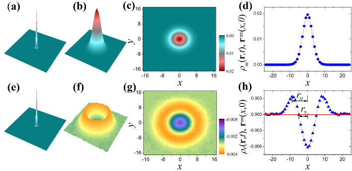
Figure 1: The diffusion of a 2D gas molecule measured by the density distribution $\rho_{m}(\mathbf{r},t)$(a)-(d) and that of the energy it carries measured by $\rho_{e}(\mathbf{r},t)$(e)-(h). Initially the molecule is located at the origin (a); $\rho_{m}(\mathbf{r},t)$ at $t=15$ is shown in (b) and its contours and intersection with $\mathbf{r}=(x,y=0)$ are shown in (c) and (d) respectively. (e)-(h) are the counterparts of (a)-(d) but for $\rho_{e}(\mathbf{r},t)$ instead.

However, surprisingly, our next study suggests the energy diffusive behavior can be significantly different. To study the energy diffusion a technical difficulty we encounter is that the energy cannot be tagged like a particle, as it will be shared and transferred among the molecules with an increasing number due to interactions. However, in this case the idea of Helfand’s ”subensemble”, i.e., the ensemble we have previously adopted by randomly selecting a molecule and setting its position as the originHelfand (4), is still valid and useful. We consider the energy distribution of the system $E(\mathbf{r},t)=H_{1}\delta(\mathbf{r}-\mathbf{r}_{1})+\sum_{i=2}^{N}H_{i}\delta(\mathbf{r}-\mathbf{r}_{i})$, where $\mathbf{r}_{i}$is the position of molecule $i$ at time $t$. In particular, we refer to the first molecule as the tagged molecule that resides on the origin initially, and focus in the following on how the total energy it bears (at time $t=0$) diffuses. For this purpose we take the ensemble average

$$\langle E(\mathbf{r},t)\rangle=\langle H_{1}\delta(\mathbf{r}-\mathbf{r}_{1})\rangle+\langle\sum_{i=2}^{N}H_{i}\delta(\mathbf{r}-\mathbf{r}_{i})\rangle,$$ (2)

which gives the energy density distribution of the system. Initially, as the origin is occupied exclusively by the tagged molecule, we have $\langle H_{1}\delta(\mathbf{r}-\mathbf{r}_{1})\rangle=\widetilde{E}\delta(\mathbf{r})$; here $\widetilde{E}=\langle H_{j}\rangle$ is the average energy of a molecule in the gas. For the rest area of the space, i.e., $\mathbf{r}\neq 0$, as it is occupied by the other $N-1$ untagged molecules uniformly, the energy density distribution they contribute to, represented by the term $\langle\sum_{i=2}^{N}H_{i}\delta(\mathbf{r}-\mathbf{r}_{i})\rangle$, equals a constant $\eta\equiv\widetilde{E}(N-1)/S$. Hence initially $\langle E(\mathbf{r},t=0)\rangle$ is characterized by a center of $\delta$-function form and a flat background. This has been well verified by the simulations (see Fig. 1(e)). As the system evolves, while the energy density distribution of the tagged molecule may spread out from its initial $\delta$-function, that of the other $N-1$ molecules is expected to be the same as $\eta$ as well. This leads to the conclusion that a reformed distribution, $\rho_{e}(\mathbf{r},t)\equiv(\langle E(\mathbf{r},t)\rangle-\eta)/\widetilde{E}$, can well capture the diffusion process of the energy the tagged molecule carries initially. This is the key point of our argument; given it the measuring of the energy diffusion of a single molecule is reduced to that of the energy density distribution of the whole system, making it possible to study the former conveniently.

Fig. 1(f) shows the energy diffusion results given by $\rho_{e}(\mathbf{r},t)$ at time $t=15$, where a distinctive difference from the molecule diffusion result of $\rho_{m}(\mathbf{r},t)$(Fig. 1(b)) can be identified. Instead of a Gaussian distribution, the function $\rho_{e}(\mathbf{r},t)$ is characterized by a growing ”crater”, i.e., a ring ridge (where $\rho_{e}(\mathbf{r},t)>0$) moves outwards leaving behind a dip (where $\rho_{e}(\mathbf{r},t)<0$) in center. (See Fig. 1(g)-(h) for the corresponding contours and the intersection with $y=0$). Two key geometric parameters of the ”crater”, denoted by $r_{\eta}$ and $r_{H}$ respectively, are the radius of the intersection ring on which $\rho_{e}(\mathbf{r},t)=0$ and that of the top ring of the ridge where $\rho_{e}(\mathbf{r},t)$ takes the maximum value (see Fig. 1(h)). We find that they depend on time linearly (see Fig. 2(a)). It should be noted that however the velocity of the ridge, represented by $\nu_{H}\equiv dr_{H}/dt$, is different from that of the opening of the dip, i.e., $\nu_{\eta}\equiv dr_{\eta}/dt$: While the former is $\nu_{H}\approx 1.1\nu_{s}$, the latter is $\nu_{\eta}\approx 0.7\nu_{s}$. Here $\nu_{s}=\sqrt{c_{p}k_{B}T}/\sqrt{c_{v}m}$ is the sound velocity in our gas model. On the other hand, as $\langle E(\mathbf{r},t)\rangle-\eta$ describes how the initial energy carried by the tagged molecule diffuses, the fact that $\rho_{e}(\mathbf{r},t)$ has a negative center suggests that, interestingly, during its diffusion some energy of the neighboring molecules is brought away in addition. This additional portion of energy is given by $-E_{-}$, where $E_{-}\equiv\widetilde{E}\int_{|\mathbf{r}|<r_{\eta}}\rho_{e}(\mathbf{r},t)d\mathbf{r}$. Similarly, the total positive energy carried by the bulk of the ridge is given by $E_{+}\equiv\widetilde{E}\int_{|\mathbf{r}|>r_{\eta}}\rho_{e}(\mathbf{r},t)d\mathbf{r}$. Due to the conversation of the energy, we have always $E_{+}+E_{-}=\widetilde{E}$. Fig2. (b) shows the time dependence of $E_{-}$ and that of $E_{+}$; initially $E_{-}$($E_{+}$) decreases (increases) but after a transition time it approach a constant. In other words, eventually the total energy brought away by the ridge is a constant and larger than the energy initially the tagged molecule carries. Together with the results of $\nu_{H}$ and $\nu_{\eta}$, they suggest clearly that rather than Gaussian, the energy diffusion follows a ballistic way resembling the process that the tsunami waves transport away the energy released from a sea earthquake.

Now let us explain why the two diffusion behaviors are so different. Consider a Brownian particle, e.g., our tagged molecule; Due to its frequent collisions with other molecules, its memory of the initial direction of motion suffers a quick loss. This process can be measured by the decay of the autocorrelation function $A(t)\equiv\langle\mathbf{p}_{1}(0)\cdot\mathbf{p}_{1}(t)\rangle$ of the tagged molecule. Here $\mathbf{p}_{i}(t)$ is the momentum of the molecule $i$ and $\mathbf{p}_{1}(t)$ is that of the tagged molecule. Indeed, the simulation suggests that $A(t)$ decreases exponentially in time in our model (not shown here), hence the motion of the tagged molecule is essentially equivalent to that of a random walker. This explains why the normal particle diffusion is observed. However, as the momentum of the tagged molecule can be transferred to other molecules during the interactions, the memory of it ”remembered” by all the molecules should thus be measured by the correlation function $M(t)\equiv\sum_{j}\langle\mathbf{p}_{1}(0)\cdot\mathbf{p}_{j}(t)\rangle$ evaluated over the whole system. Dividing the momentum of a molecule, say molecule $j$, into two parts: $\mathbf{p}_{j}(t)=\mathbf{p}_{j}^{\prime}(t)+\mathbf{p}_{j}^{\prime\prime}(t)$, where $\mathbf{p}_{j}^{\prime}(t)$($\mathbf{p}_{j}^{\prime\prime}(t)$) represents the momentum transferred to it from the tagged molecule (other molecules), we then have $M(t)=\sum_{j}\langle\mathbf{p}_{1}(0)\cdot\mathbf{p}_{j}^{\prime}(t)\rangle=\langle\mathbf{p}_{1}(0)\cdot\mathbf{p}_{1}(0)\rangle$; This is because (1) $\langle\mathbf{p}_{1}(0)\cdot\mathbf{p}_{j}^{\prime\prime}(t)\rangle=0$ since $\mathbf{p}_{j}^{\prime\prime}(t)$ is independent of $\mathbf{p}_{1}(0)$ and (2) $\sum_{j}\mathbf{p}_{j}^{\prime}(t)=\mathbf{p}_{1}(0)$ since the momentum $\mathbf{p}_{1}(0)$ is conserved in the system. This result that $M(t)$ is in fact a time-independent constant suggests that, though the information of its initial state will be forgotten quickly by a molecule itself, it will always be remembered by others. Hence it is in effect not lost.

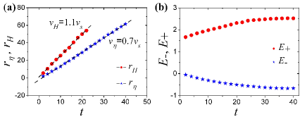
Figure 2: (a) The time dependence of the characterizing radii, corresponding to the top ring of the ridge (red bullets) and the opening of the center dip (black stars), respectively. The best fittings (dashed lines) suggest their expending speeds $\nu_{H}\approx 1.1\nu_{s}$ and $\nu_{\eta}\approx 0.7\nu_{s}$. (B) The positive and negative potion of energy, $E_{+}$(red bullets) and $E_{-}$(black stars), corresponding to the integrated energy density distribution over region $|\mathbf{r}|>r_{\eta}$ and $|\mathbf{r}|<r_{\eta}$ respectively.

In Fig. 3 presents the simulation results of $\rho_{m}(\mathbf{r},t)$ and $\rho_{e}(\mathbf{r},t)$ for an ensemble where the momentum direction of the tagged molecule is normalized as well. Unlike in the study presented in Fig. 1, where for each random realization the tagged molecule has a momentum with random direction and hence the memory effects of the direction are hidden, here we instead reset (renormalize) the direction of the initial momentum of the tagged molecule to be the same as the axis $y$. This is equivalent to considering a subset of the Helfand subensemble where the direction of the momentum of the considered molecule is specified as well. As such the tagged molecule will keep going along axis $y$ in a short initial stage. It can be seen from Fig. 3 that while $\rho_{m}(\mathbf{r},t)$ is isotropic, implying a memory loss effect, $\rho_{e}(\mathbf{r},t)$ is obviously anisotropic, showing a strong signal of the initial moving direction of the tagged molecule.

Because the memory is kept during the momentum diffusion and thus the energy diffusion process (as the energy is transferred simultaneously with the momentum), the energy diffusion cannot be a Markov process. This explains why it shows an abnormal diffusion behavior. However, at present we cannot explain yet why the diffusion is ballistic, which calls for further studies in future. It should be noted that in the macroscopic world the ballistic transport of energy has been found ubiquitous. For example, it is in a ballistic way that the shock waves bring away the energy of an explosion, and so do the sea waves in a tsunami to bring away the energy from a sea earthquake. Even in a much more ”peaceful” case like dropping a pebble into a pond, it is the way that partial kinetic energy of the pebble is carried away by the homocentric ripples. In all these examples, it is certain that the bulk of the excited energy is transported by waves. Our finding in this Letter implies that the wave could also be a general energy transporting approach on the microscopic level, i.e., on a single molecule level as exposed here. The only differences of our finding from the macroscopic examples cited above lies in that our results are based on the ensemble average.

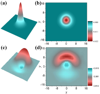
Figure 3: The density distributions of a 2D gas particle $\rho_{m}(\mathbf{r},t)$(a)-(b) and the related energy density distribution $\rho_{e}(\mathbf{r},t)t=15$(c)-(d). Initially the particle is located at origin, and its velocity direction is renormalized to be the same as axis $y$. The right column is the contours plot of the corresponding figure in left column. $3\times 10^{8}$random realizations are considered for ensemble average.

In summary, we have shown numerically that the energy carried by a molecule in a 2D gas may spread out in a ballistic way at room temperature. Considering the ensemble average, the energy profile is found to be characterized by a ring ridge and a dip in center, and both expand outward with constant speeds. As a basic mechanism of the energy transportation in gas, we believe this property may find important applications. For example, one possible situation is the Tokamak plasma, where the heat conductivity has been found to deviate significantly from the prediction based on classical normal diffusion theoriesChen-f-f (12). Our finding provides a new perspective for revisiting such challenging problems.

This work is supported by the National Natural Science Foundation of China under Grant No. 10775115, 10925525, and the National Basic Research Program of China (973 Program) (2007CB814800).

References

- (1) A. Einstein, Annalen der Physik 17, 549-560 (1905).
- (2) M. von Smoluchowski, Annalen der Physik 21, 756-780 (1906).
- (3) M. S. Bello, R. Rezzonico, and P. G. Righetti, Science 266, 773-776 (1994); E. L. Cussler, Diffusion: Mass Transfer in Fluid Systems (Cambridge University Press, 1997); T.R Marrero, Gaseous Diffusion Coefficients (American Chemical Society and the American Institute of Physics for the National Bureau of Standards, ([Washington]), 1972).
- (4) Eugene Helfand, Phys. Rev. 119, 1 (1960).
- (5) Melville S. Green, J. Chem. Phys. 19, 1036-1046 (1951).
- (6) Melville S. Green, Phys. Rev. 119, 829 (1960).
- (7) R. Kubo, J. Phys. Soc. Jpn. 12, 570-586 (1957).
- (8) S. Viscardy, J. Servantie, and P. Gaspard, J. Chem. Phys. 126, 184512-7 (2007).
- (9) S. Viscardy, J. Servantie, and P. Gaspard, J. Chem. Phys. 126, 184513-5 (2007).
- (10) L. Landau, J. Phys. (USSR) 5, 51 (1941); D. Ter Haar, Collected Papers of L. D. Landau (Intl Pub Distributor Inc, 1965).
- (11) B. J. Alder and T. E. Wainwright, Phys. Rev. A 1, 18 (1970).
- (12) F. F. Chen, Introduction to Plasma Physics and Controlled Fusion: Plasma Physics (Springer, 1984).