Critical frontier of the Potts and percolation models on triangular-type and kagome-type lattices I: Closed-form expressions

Abstract

We consider the Potts model and the related bond, site, and mixed site-bond percolation problems on triangular-type and kagome-type lattices, and derive closed-form expressions for the critical frontier. For triangular-type lattices the critical frontier is known, usually derived from a duality consideration in conjunction with the assumption of a unique transition. Our analysis, however, is rigorous and based on an established result without the need of a uniqueness assumption, thus firmly establishing all derived results. For kagome-type lattices the exact critical frontier is not known. We derive a closed-form expression for the Potts critical frontier by making use of a homogeneity assumption. The closed-form expression is new, and we apply it to a host of problems including site, bond, and mixed site-bond percolation on various lattices. It yields exact thresholds for site percolation on kagome, martini, and other lattices, and is highly accurate numerically in other applications when compared to numerical determination.

I Introduction

An outstanding problem in lattice statistics is the determination of the critical frontier, or the loci of critical point, of lattice models. Of special interest is the $q$-state Potts model potts52 and its associated lattice models wureview . For $q=2$ it is the Ising model, and for $q=1$ the Potts model generates the percolation problem wu1978 including the bond kas , site kw , ane mixed site-bond percolation. However, except for the simple square, triangular and honeycomb lattices wu79 and some special lattices essentially of a triangular-type wupotts06 , the determination of the Potts critical frontier in general has proven to be elusive.

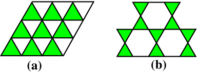
Figure 1: (a) Triangular-type lattice. (b) Kagome-type lattice. Shaded triangles possess Boltzmann weights (1).

In this paper we consider the Potts model on two general classes of lattices, the triangular- and kagome-type lattices shown in Fig. 1. Shaded triangles in Fig. 1 denote interactions involving 3 Potts spins $\tau_{1},\tau_{2},\tau_{3}=1,2,...,q$ with the Boltzmann weights

$$W_{\bigtriangleup}(1,2,3) = A+B(\delta_{12}+\delta_{23}+\delta_{31})+C\delta_{123}\,,$$

$$W_{\bigtriangledown}(1,2,3) = A^{\prime}+B^{\prime}(\delta_{12}+\delta_{23}+\delta_{31})+C^{\prime}\delta_{123}\,,$$ (1)

where $\delta_{ij}=\delta_{\rm Kr}(\tau_{i},\tau_{j}),\delta_{123}=\delta_{12}\,\delta_{23}\,\delta_{31}$, and $A,B,C,A^{\prime},B^{\prime},C^{\prime}$ are constants. In (1), we have assumed interactions isotropic in the 3 directions of a triangle. The extension of our analysis to anisotropic interactions is straightforward and will not be given. Special cases of shaded triangles are the “stack-of-triangle”, or subnet, lattices shown in Figs. 2 and 3 that have been of recent interest yao08 ; loh08 ; ziffgu09 ; HAZiff09 . We refer to these stack-of-triangle lattices as subnet lattices. The $1\times 1$ subnet lattices are the triangular and kagome lattices themselves. We shall call a kagome-type lattice with  $m\times m$  down-pointing and  $n\times n$  up-pointing subnets an  $(m\times m):(n\times n)$  subnet lattice, or simply an  $(m\times m):(n\times n)$  lattice. Examples of these kagome-type subnet lattices are shown in Fig. 3.

Figure 2: Triangular subnet lattices. (a) $1\times 1$ lattice (triangular). (b) $2\times 2$ lattice. (c) $3\times 3$ lattice.

Figure 3: Kagome subnet lattices. (a) $(1\times 1):(1\times 1)$ lattice (kagome). (b) $(2\times 2):(2\times 2)$  lattice. (c) $(3\times 3):(3\times 3)$   lattice. (d) $(1\times 1):(2\times 2)$  lattice.

Partition functions for the two lattices in Fig. 1 are

$$Z_{\rm tri}(q;A,B,C) = \sum_{\tau_{i}=1}^{q}\prod_{\bigtriangleup}W_{\bigtriangleup}(i,j,k)\,,$$ (2)

$$Z_{\rm kag}(q;A,B,C;A^{\prime},B^{\prime},C^{\prime}) = \sum_{\tau_{i}=1}^{q}\big{[}\prod_{\bigtriangleup}W_{\bigtriangleup}(i,j,k)\big{]}\cdot\big{[}\prod_{\bigtriangledown}W_{\bigtriangledown}(i^{\prime},j^{\prime},k^{\prime})\big{]},$$ (3)

where the products are taken over the respective up- and down-pointing shaded triangles. The critical frontier of the triangular-type lattice of Fig. 1(a) has been known from earlier works bta78 ; wulin80 ; wuzia81 , but the critical frontier for the kagome-type lattice of Fig. 1(b) is open.

For $q=2$, we can replace Potts spins $\tau$ by Ising spins $\sigma=\pm 1$ and shaded triangles by triangles ($1\times 1$ subnet) with an Ising interaction $K_{I}$ $(=K/2)$. To determine $K_{I}$, we write

$$\delta_{ij} = \frac{1}{2}(1+\sigma_{i}\sigma_{j}),$$

$$W_{\bigtriangleup}(1,2,3) = {\rm exp}[2K_{I}(\delta_{12}+\delta_{23}+\delta_{31})].$$ (4)

Equating (4) with $W_{\bigtriangleup}$ in (1), one obtains after a little algebra

$$e^{4K_{I}}=(A+3B+C)/(A+B).$$ (5)

It follows that the partition functions (2) and (3) are completely equivalent to those of the triangular and kagome Ising model.

For $q\geq 3$, the shaded triangles can be replaced by any triangular network having 2 independent parameters. An example is the mapping shown in Fig. 12 in Sec. III.7.

Parameters $A,B,C$ for a given Potts subnet can be readily worked out. For the $1\times 1$ triangle, for example, one has

$$W_{\bigtriangleup}(1,2,3)={\rm exp}[K(\delta_{12}+\delta_{23}+\delta_{31})]$$ (6)

from which one obtains

$$A=1,\quad B=v,\quad C=3v^{2}+v^{3},\quad\quad({\rm triangle}),$$ (7)

where $v=e^{K}-1$. For the $2\times 2$ subnet, one obtains in a similar fashion

$$A = 3v^{5}+21v^{4}+(50+4q)v^{3}+33qv^{2}+9q^{2}v+q^{3},$$

$$B = v^{7}+7v^{6}+22v^{5}+(30+2q)v^{4}+10qv^{3}+q^{2}v^{2},$$

$$C = v^{9}+9v^{8}+33v^{7}+63v^{6}+(54+3q)v^{5}+9qv^{4},\quad\quad(2\times 2{\rm\>\>subnet)}.$$ (8)

Expressions of $A,B,C$ for $3\times 3$ and $4\times 4$ subnets are derived and given in a subsequent paper II , hereafter referred to as II.

The structure of this paper is as follows: In Sec. II we consider the triangular subnet lattices and apply the rigorously known critical frontier to various models including mixed site-bond percolation. In Sec. III we consider the kagome-type lattice, and derive a closed-form expression for its critical frontier on the basis of a homogeneity assumption. We show that this critical frontier is exact for site percolation on the kagome, martini, and other lattices, and is highly accurate in other applications. The accuracy of the critical frontier will be closely examined in paper II.

II Triangular-type lattices

In this section we consider triangular-type lattices of Fig. 1(a).

The Potts model on the triangular-type lattice was first studied by Baxter, Temperley and Ashley bta78 in the context of a Potts model with 2- and 3-site interactions. Using a Bethe-ansatz result on a 20-vertex model on the triangular lattice due to Kelland kelland1 ; kelland2 , they showed that the partition function (2) is self-dual, and derived its self-dual point which, in the language of the interaction (1), reads

$$qA=C.$$ (9)

This self-dual trajectory was later re-derived graphically by Wu and Lin wulin80 . However, as is common in duality arguments, an additional assumption of a unique transition is needed to ascertain that (9) is indeed the actual critical frontier.

However, Wu and Zia wuzia81 established subsequently in a rigorous analysis that (9) is indeed the critical frontier in the ‘ferromagnetic’ regime

$$2B+C>0,\quad 3B+C>0.$$ (10)

It can be verified that the condition (10) holds for (7) and (8), so the critical frontier $qA=C$ is exact. Applications of (9) to the martini and other lattices have been reported in wupotts06 . The duality relation of the triangular Potts model with 2- and 3-spin interactions has also be studied by Chayes and Lei chayeslei06 with several rigorous theorems on the phase transition proven.

II.1 Ising model

In Sec. I, we have established that for $q=2$ any triangular-type lattice is reducible to a triangular Ising lattice with interaction $K_{I}$ given by (5). Indeed, using (5), the known critical point $e^{4K_{I}}=3$ of the triangular Ising model reduces to the critical frontier $2A=C$ as expected.

For the Ising model on  $1\times 1$  and  $2\times 2$  subnet lattices with interaction $K_{I}$, we set $q=2$, $v=e^{2K_{I}}-1$ in (7) and (8), and obtain from $2A=C$ the critical point

$$x_{c} = \sqrt{3},\quad 1\times 1{\rm\>\>subnet\>(triangular\>lattice)}$$ (11)

$$= \sqrt{5},\quad 2\times 2{\rm\>\>subnet},$$

where $x=e^{2K_{I}}$. Using expressions of $A$ and $C$ given in II for  $3\times 3$  and  $4\times 4$  subnets, we obtain similarly

$$x^{8}-5x^{6}-x^{4}-19x^{2}-8=0,\quad x_{c} = \frac{1}{2}\sqrt{5+\sqrt{33}+\sqrt{(50+18\sqrt{33})}}$$

$$= 2.404\ 689\ 372,\ 3\times 3{\rm\>subnet}$$

$$x^{12}-5x^{10}-x^{8}-22x^{6}-53x^{4}-125x^{2}-51=0,\quad x_{c} = 2.467\ 648\ 033,\ 4\times 4{\rm\>subnet}.$$ (12)

II.2 Bond percolation

It is well-known that bond percolation is realized in the $q=1$ limit of the Potts model under the mapping $v=p/(1-p)$, where $p$ is the bond occupation probability kas ; wu1978 . Therefore the percolation threshold is given simply by $C=A$. Thus using (7) for $A$ and $C$ for the triangular lattice, one obtains the well-known sykesessam ; essam72 ; essam79 critical frontier for bond percolation

$$1-3p+p^{3}=0,\quad{\rm or}\quad p_{c}=2\sin(\pi/{18})=0.347\ 296\ 355.\quad{\rm(triangular\>lattice)}.$$ (13)

For the $2\times 2$ subnet lattice we use (8) and obtain

$$1-3p^{2}-9p^{3}+3p^{4}+45p^{5}-72p^{6}+45p^{7}-12p^{8}+p^{9}=0,$$

$$\hskip 56.9055pt{\rm or}\quad p_{c}=0.471\ 628\ 788\quad(2\times 2{\rm\>subnet\>\>lattice}).$$ (14)

In a similar fashion using expressions of $A$ and $C$ given in II, we obtain

$$1-3p^{3}-18p^{4}-39p^{5}+77p^{6}+309p^{7}-198p^{8}-1406p^{9}+315p^{10}+9303p^{11}-23083p^{12}$$

$$\hskip 28.45274pt+28707p^{13}-22047p^{14}+10959p^{15}-3462p^{16}+636p^{17}-52p^{18}=0,$$

$$\hskip 85.35826ptp_{c}=0.509\ 077\ 792\quad\quad(3\times 3{\rm\>\>subnet\>\>lattice}),$$ (15)

$$1-3p^{4}-30p^{5}-114p^{6}-63p^{7}+636p^{8}+1940p^{9}+741p^{10}-14283p^{11}-26541p^{12}$$

$$+78759p^{13}+189279p^{14}-370589p^{15}-1229877p^{16}+2829339p^{17}+6938691p^{18}-41655363p^{19}$$

$$+96750306p^{20}-143421123p^{21}+152405700p^{22}-121438416p^{23}+73822093p^{24}-34270647p^{25}$$

$$+11994555p^{26}-3073478p^{27}+545409p^{28}-60012p^{29}+3089p^{30}=0,$$

$$\hskip 85.35826ptp_{c}=0.524\ 364\ 822\quad\quad(4\times 4{\rm\>\>subnet\>\>lattice}).$$ (16)

These findings agree with those of Haji-Akbari and Ziff HAZiff09 deduced from a duality consideration. As aforementioned, our derivation now ascertains that these thresholds are the exact transition points.

II.3 Potts model

The exact critical threshold for the Potts model on triangular-type lattices is (9), or $qA=C$. Using expressions of $A$ and $C$ given in (7), one obtains the known critical frontier kimjoseph ; wu79

$$3v^{2}+v^{3}=q,\quad\quad({\rm Potts\>\>model\>\>on\>\>triangular\>\>lattice}).$$ (17)

For the $2\times 2$ subnet lattice one uses (8) and obtains the critical frontier

$$v^{9}+9v^{8}+33v^{7}+63v^{6}+54v^{5}-12qv^{4}-(50q+4q^{2})v^{3}-33q^{2}v^{2}-9q^{3}v-q^{4}=0.$$ (18)

Solutions of (17) and (18) and those of the  $3\times 3$  and  $4\times 4$  subnet lattices are tabulated in Table 1 for $q=1,2,3,4,10$. Note that the $q=1$ solutions are related to the bond percolation thresholds (13)-(16) by $e^{K_{c}}=1/(1-p_{c})$.

Table 1: Exact Potts threshold $e^{K_{c}}$ for triangular-type subnet lattices.

	$q=1$	$q=2$ (Ising)	$q=3$	$q=4$	$q=10$
Triangular lattice	1.532 088 885	$\sqrt{3}$	1.879 385 241	2	2.492 033 301
$2\times 2$	1.892 608 790	$\sqrt{5}$	2.493 123 120	2.706 275 430	3.602 637 947
$3\times 3$	2.036 982 609	2.404 689 372	2.674 398 828	2.895 419 068	3.808 005 450
$4\times 4$	2.102 451 724	2.467 648 033	2.731 876 784	2.946 645 097	3.820 754 228

II.4 Site percolation

Kunz and the present author kw have shown that site percolation can be formulated as a $q=1$ limit of a Potts model with multi-site interactions. The Kunz-Wu scheme is to consider a reference lattice with multi-spin interactions, and regard faces of multi-spin interactions as sites of a new lattice on which the site percolation is defined. The critical frontier of the Potts model on the reference lattice then produces the site percolation threshold for the new lattice. This scheme of formulation can be extended to mixed site-bond percolation.

1. Site percolation on the triangular lattice:

Consider as a reference lattice the triangular lattice with pure 3-site interactions $M$ marked by dots shown in the left panel of Fig. 4. The dots form a triangular lattice shown in the right. The Kunz-Wu scheme now solves the site percolation on the triangular lattice. We have

$$W_{\bigtriangleup}(1,2,3)=e^{M\delta_{123}}=1+m\,\delta_{123}\,,$$ (19)

or $A=1,\,B=0,\,C=m=e^{M}-1$. Writing $m=s/(1-s)$, where $s=1-e^{-M}$ is the site occupation probability, the exact critical frontier $A=C$ now yields immediately the well-known site percolation threshold sykesessam ; essam72 ; essam79 ; sudingziff99 for the triangular lattice,

$$s_{c}=1/2\,.$$ (20)

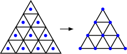
Figure 4: Site percolation on the triangular lattice.

2. Site percolation on kagome lattice:

Consider the reference $2\times 2$ subnet lattice with pure 3-site interactions $M$ denoted by dots shown in the left panel of Fig. 5. The Kunz-Wu scheme then maps the reference Potts model into site percolation on the kagome lattice as indicated in the right.

Now for a  $2\times 2$  subnet containing 3 dots as in Fig. 5, we have

$$A=q^{3}+3\,qm,\quad B=m^{2},\quad C=m^{3},$$ (21)

where $m=e^{M}-1$. Writing $m=s/(1-s)$ and setting $q=1$, the rigorous critical frontier $A=C$ yields the critical condition $1-3s^{2}+s^{3}=0$, leading to the known exact result sykesessam ; essam72

$$s_{c}^{kag}=1-2\sin(\pi/18)=0.652\ 703\ 644.$$ (22)

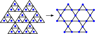
Figure 5: Site percolation on the kagome lattice.

3. Site percolation on  $(1\times 1):(n\times n)$   lattices:

The above scheme of mapping can be extended to site percolation on  $(1\times 1):(n\times n)$  lattices for general $n$. The example of Fig. 5 is $n=1$, and the $n=2$ lattice is shown in Fig. 6. The reference lattice (not shown) for $n=2$ consists of  $3\times 3$  subnets with

$$A = q^{7}+6q^{5}m+15q^{3}m^{2}+(14q+3q^{2})m^{3}+3m^{4},$$

$$B = q^{2}m^{3}+2(q+1)m^{4}+m^{5},$$

$$C = 3m^{5}+m^{6},$$ (23)

where $m=e^{M}-1$, $M$ is the 3-site interaction. After setting $q=1$ and $m=s/(1-s)$, the critical frontier $qA=C$ becomes

$$(1-2s^{2})(1+2s^{2}-3s^{3}+s^{4})=0,$$ (24)

yielding the exact threshold

$$s_{c}=1/\sqrt{2},\quad\quad(1\times 1):(2\times 2){\rm\>\>kagome\>\>site\>\>percolation}.$$ (25)

The exact critical threshold for higher  $(1\times 1):(n\times n)$ lattices can be similarly worked out.

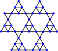
Figure 6: Site percolation on the  $(1\times 1):(2\times 2)$   lattice.

III Kagome-type lattices

We consider in this section the case of the kagome-type lattices of Fig. 1(b).

The critical frontier of the Potts model on kagome-type lattices has proven to be highly elusive. On the basis of a homogeneity assumption, however, the present author wu79 has advanced a conjecture on the critical point for the kagome lattice. The conjecture has since been closely examined wuhu ; ziffsuding97 ; scullardziff ; fengdengbloete08 and found to be extremely accurate. Here we extend the homogeneity assumption to general kagome-type Potts lattices. For continuity of reading, we first state our result in Sec. III.1, and present the derivation in Sec. III.7.

III.1 A closed-form critical frontier and homogeneity assumption

For Potts model on kagome-type lattices described by the partition function (3), the critical frontier under a homogeneity assumption is

$$(q^{2}A+3q\,B+C)(q^{2}A^{\prime}+3q\,B^{\prime}+C^{\prime})-3(qB+C)(qB^{\prime}+C^{\prime})-(q-2)CC^{\prime}=0.$$ (26)

Remarks:

1. Despite its appearance, the critical frontier (26) actually contains only 3 independent parameters (Cf. (55) below).

2. The expression (26) is exact for $q=2$.

III.2 Ising model

We first show that (26) is exact for $q=2$. We have already established that the partition function (3) is precisely that of the kagome Ising model. For completeness we now verify that the critical frontier (26) also gives the known kagome critical point.

For symmetric weights $A=A^{\prime},B=B^{\prime},C=C^{\prime}$, the kagome Ising model has a uniform interaction $K_{I}$ and the critical point is known to be at $e^{4K_{I}}=3+2\sqrt{3}$ syozi . It is readily verified that, by using (5) for $K_{I}$, this critical point gives rise to precisely the $q=2$ critical frontier (26), namely,

$$4A+6B+C=\sqrt{3}\,(2B+C).$$ (27)

The proof can be extended to the kagome-type model with asymmetric weights.

Critical thresholds of kagome-type Ising subnet lattices computed from (27) are tabulated in Table 3. For the kagome and  $(2\times 2):(2\times 2)$  Ising lattices, for example, we use (7) and (8) for $A,B,C$ with $q=1,\,v=x-1,\,x=e^{2K_{I}}$. This gives

$$x^{4}-6x^{2}-3=0,\quad x_{c} = \sqrt{3+2\sqrt{3}}$$

$$= 2.542\ 459\ 756,\quad\quad\quad{\rm(kagome\>lattice)},$$

$$x^{8}-8x^{6}-6x^{4}-32x^{2}-83=0,\quad x_{c} = \sqrt{2+\sqrt{3}+\sqrt{12+10\sqrt{3}}}$$ (28)

$$= 3.024\ 382\ 957,\quad(2\times 2):(2\times 2){\rm\>\>lattice}.$$

III.3 Bond percolation

Table 2: Bond percolation threshold $p_{c}$ for  $(m\times m):(n\times n)$   lattices for $m,n\leq 4$.

Lattice	This work	Numerical determination
Kagome	0.524 429 717	0.524 404  99(2) fengdengbloete08
($1\times 1):(2\times 2)$	0.570 882 620	0.570 866 51(33) ziffgu0910
$(1\times 1):(3\times 3)$	0.599 798 340
$(1\times 1):(4\times 4)$	0.592 017 120
$(2\times 2):(2\times 2)$	0.600 870 248	0.600 862 4(10) ziffgu09
$(2\times 2):(3\times 3)$	0.610 916 740
$(2\times 2):(4\times 4)$	0.614 703 624
$(3\times 3):(3\times 3)$	0.619 333 485	0.619 329 6(10) ziffgu09
$(3\times 3):(4\times 4)$	0.622 473 191
$(4\times 4):(4\times 4)$	0.625 364 661	0.625 365 (3) ziffgu09

For bond percolation threshold on kagome-type subnet lattices, we again use (26) with the substitution of $q=1$ and $v=p/(1-p)$, where $p$ is the bond occupation probability. Using (7) and (8), we obtain

$$1-3p^{2}-6p^{3}+12p^{4}-6p^{5}+p^{6}=0,\quad p_{c}=0.524\ 429\ 717{\rm\>\>(kagome\>\>lattice)},$$ (29)

$$1-3p^{3}-12p^{4}-12p^{5}+63p^{6}+60p^{7} - 330p^{8}+423p^{9}-264p^{10}+84p^{11}-11p^{12}=0,$$

$$p_{c} = 0.570\ 882\ 620,\quad(1\times 1):(2\times 2){\rm\>\>lattice},$$ (30)

$$1-3p^{4}-18p^{5}-39p^{6}+30p^{7} + 273p^{8}+264p^{9}-1785p^{10}-126p^{11}+8232p^{12}-16236p^{13}$$

$$+ 16359p^{14}-9948p^{15}+3708p^{16}-786p^{17}+73p^{18}=0,$$

$$p_{c} = 0.600\ 870\ 248,\quad(2\times 2):(2\times 2){\rm\>\>lattice}.$$ (31)

Bond percolation thresholds computed from (26) for  $(m\times m):(n\times n)$   lattices are tabulated in Table 2. We also include in Table 2 numerical determinations of $p_{c}$ for the  $(1\times 1):(2\times 2)$ ziffgu0910 and  $(n\times n)\times(n\times n)$, $n=2,3,4$ ziffgu09 lattices by Ziff and Gu using simulations, and of the kagome lattice by Feng, Deng and Blöte fengdengbloete08 from a transfer matrix analysis. The comparison shows that (26) is accurate to within one part in $10^{5}$.

III.4 Potts model

Table 3: Potts threshold $e^{K_{c}}$ for kagome-type subnet lattices.

Lattice	$q=1$	$q=2$ (Ising)	$q=3$	$q=4$	$q=10$
kagome lattice	2.102 738 619	2.542 459 757	2.876 269 226	3.155 842 236	4.355 385 241
$(1\times 1):(2\times 2)$	2.330 364 713	2.821 281 889	3.186 678 923	3.489 096 458	4.761 529 399
$(1\times 1):(3\times 3)$	2.498 740 260	2.903 273 662	3.260 483 758	3.553 390 863	4.764 908 410
$(1\times 1):(4\times 4)$	2.451 083 242	2.928 442 860	3.276 998 285	3.562 314 883	4.739 553 252
$(2\times 2):(2\times 2)$	2.505 450 909	3.024 382 957	3.481 055 307	3.717 691 692	5.016 332 520
$(2\times 2):(3\times 3)$	2.570 143 984	3.082 166 484	3.454 087 416	3.757 519 846	5.004 155 712
$(2\times 2):(4\times 4)$	2.595 404 635	3.098 624 716	3.378 293 046	3.761 399 505	4.984 524 206
$(3\times 3):(3\times 3)$	2.626 971 274	3.133 002 727	3.497 087 416	3.712 498 867	4.992 841 134
$(3\times 3):(4\times 4)$	2.648 818 511	3.147 204 863	3.416 364 328	3.796 037 357	4.973 931 010
$(4\times 4):(4\times 4)$	2.669 262 336	3.160 721 132	3.598 289 910	3.639 241 821	4.954 642 401

Critical thresholds for the Potts model on kagome-type subnet lattices computed from (26) are tabulated in Table 3. For the kagome lattice itself, for example, we have $A=A^{\prime}=1,B=B^{\prime}=v,C=C^{\prime}=3v^{2}+v^{3},v=e^{K}-1$, and (26) gives the critical frontier

$$v^{6}+6v^{5}+9v^{4}-2qv^{3}-12qv^{2}-6q^{2}v-q^{3}=0,\quad\quad{\rm(kagome\>lattice)}.$$ (32)

The critical frontier (32) for the kagome lattice was first obtained by the present author some 30 years ago wu79 ; remark by using the homogeneity assumption described in Sec. III.7. Comparison of the thresholds computed from (32) for $q=1,3,4$ with Monte Carlo renormalization group findings has shown that the accuracy of (26) is within one part in $10^{5}$ wuhu .

III.5 Site and site-bond percolation

We now apply (26) to site as well as mixed site-bond percolation. First we show that (26) is exact in some instances.

1. Site percolation on the 3-12 and kagome lattices.

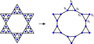
Figure 7: Site percolation on the 3-12 lattice.

The 3-12 lattice is the lattice shown in the right panel of Fig. 7. To formulate site percolation on the 3-12 lattice, we consider the reference  $(2\times 2):(2\times 2)$   lattice with pure 3-site interactions shown in the left. Let the 3-site interactions of the up- and down-triangles be, respectively, $M_{1}$ and $M_{2}$. One finds

$$A = q^{3}+3\,qm_{1},\quad B=m_{1}^{2},\quad C=m_{1}^{3},$$

$$A^{\prime} = q^{3}+3\,qm_{2},\quad B^{\prime}=m_{2}^{2},\quad C^{\prime}=m_{2}^{3},$$ (33)

where $m_{1}=e^{M_{1}}-1$, $m_{2}=e^{M_{2}}-1$. Setting $q=1$, $m_{1}=s_{1}/(1-s_{1})$, $m_{2}=s_{2}/(1-s_{2})$, where $s_{1}$ and $s_{2}$ are the respective site occupation probabilities for the 3-12 lattice, the critical frontier (26) gives

$$1-3(s_{1}s_{2})^{2}+(s_{1}s_{2})^{3}=0,\quad\quad(3-12{\rm\>\>site\>\>percolation}).$$ (34)

For $s_{1}=s_{2}=s$, this yields the known sykesessam ; sudingziff99 critical frontier $1-3s^{4}+s^{6}=0$, or

$$s_{c}^{3-12}=\sqrt{1-2\sin(\pi/18)}=0.807\ 900\ 076.$$ (35)

Using the relation $s_{c}^{kag}=\big{(}s_{c}^{3-12}\big{)}^{2}$ sudingziff99 , we have therefore derived the exact kagome and 3-12 site percolation thresholds, and demonstrated that (26) is exact in this instance.

2. Site percolation on the martini lattice.

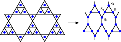
Figure 8: Site percolation on the martini lattice.

The martini lattice scullard06 is the lattice shown in the right panel of Fig. 8. To generate a site percolation on the martini lattice, we start from the  $(1\times 1):(2\times 2)$  reference lattice with 3-site interactions shown in the left. Denote the 3-site interactions of up- and down-pointing triangular faces by $M_{1}$ and $M_{2}$ respectively and write $m_{1}=e^{M_{1}}-1$, $m_{2}=e^{M_{2}}-1$. We have

$$A = q^{3}+3\,qm_{1},\quad B=m_{1}^{2},\quad C=m_{1}^{3}$$

$$A^{\prime} = 1,\hskip 56.9055pt\ B^{\prime}=0,\quad\ \ C^{\prime}=m_{2}.$$ (36)

Setting $q=1$, $m_{1}=s_{1}/(1-s_{1}),\,m_{2}=s_{2}/(1-s_{2}),$ with $s_{1}$ and $s_{2}$ the respective site occupation probabilities, (26) gives the critical frontier

$$1-(3\,s_{1}^{2}-s_{1}^{3})s_{2}=0,\quad\quad({\rm martini\>\>site\>\>percolation}).$$ (37)

This is a known exact result scullardziff ; kondor ; ziff06 , and is another example that the critical frontier (26) is exact. For $s_{2}=1$, the percolation reduces to that on the kagome lattice, and (37) gives the threshold (22). For uniform occupation probability $s_{1}=s_{2}=s$, (37) becomes $1-3s^{3}+s^{4}=0$ and gives the exact solution $s_{c}^{martini}=0.764\ 826\ 486$.

3. Site-bond percolation on the honeycomb lattice.

No exact result is known for the site and site-bond percolation on the honeycomb lattice. Owing to the intrinsic interest of a percolation process on a simple Bravais lattice, the problem of honeycomb site percolation has attracted considerable attention for many years. There now exists a host of highly precise numerical estimates on the threshold for site percolation on the honeycomb lattice sudingziff99 ; ziffgu09 ; fengdengbloete08 .

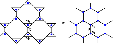
Figure 9: Site-bond percolation on the honeycomb lattice.

Consider the more general mixed site-bond percolation on the honeycomb lattice with site occupation probabilities $s_{1}$ and $s_{2}$ and bond occupation probability $p$ shown in the right panel of Fig. 9. The relevant reference lattice can be taken as shown in the left with edge-interactions $K$ and 3-site interactions $M_{1}$ and $M_{2}$. To make use of (26), we adopt the scheme of devising up- and down-pointing triangles as indicated in Fig. 11(b) below. This gives

$$A = (q+v)^{3}+(q+3v)m_{2},\quad B=v^{2}m_{2},\quad C=v^{3}m_{2},$$

$$A^{\prime} = 1,\hskip 116.65646ptB^{\prime}=0,\quad\quad\>C^{\prime}=m_{1},$$ (38)

where $v=e^{K}-1,m_{i}=e^{M_{i}}-1,i=1,2$. Setting $q=1,v=p/(1-p),m_{i}=s_{i}/(1-s_{i})$, we obtain from (26) the critical frontier for the mixed site-bond percolation as

$$(3p^{2}-p^{3})s_{1}s_{2}=1,\quad\quad({\rm honeycomb\>\>site-bond\>\>percolation}).$$ (39)

When $s_{1}=s_{2}=1$, (39) is exact since it gives the known honeycomb bond percolation threshold $1-3p^{2}+p^{3}=0$ sykesessam ; essam72 ; essam79 . When $p=1$, (39) gives the threshold

$$s_{1}s_{2}=1/2$$ (40)

which is exact for $s_{2}=1$, as the site percolation reduces to one on the triangle lattice with the critical point (20) $s_{c}=1/2$. But for $s_{1}=s_{2}=s$, (40) gives $s_{c}=1/\sqrt{2}=0.707\ 106\ 781$ differing from accurate numerical estimates of $s_{c}=0.697\ 040\ 2$ fengdengbloete08 and $s_{c}=0.697\ 041\ 3$ ziffgu09 . The critical frontier (26) is therefore a close approximation in this instance.

The site-bond percolation has also been studied by simulations by Ziff and Gu for $s_{1}=s_{2}$ ziffgu09 and for $p=1$ ziffgu0910 . Their results indicate (39) works better for site occupation probabilities $\sim 1$.

4. Site-bond percolation on the kagome lattice.

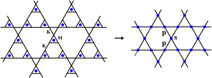
Figure 10: Site-bond percolation on the kagome lattice.

Consider the mixed site-bond percolation on the kagome lattice with site and bond occupation probabilities $s$ and $p$ shown in the right panel of Fig. 10. The reference lattice is shown in the left having edge interaction $K$ and 3-site interaction $M$. Regard the reference lattice as a kagome-type with the partition function (3). One has

$$A = q(q^{2}+3m)(q+v)^{3}+3m^{2}(q+v)^{2}+m^{3},$$

$$B = m^{2}(q+v)^{2}+m^{3}v,$$

$$C = m^{3}(3v^{2}+v^{3}),$$

$$A^{\prime} = 1,\quad\quad B^{\prime}=v,\quad\quad C^{\prime}=3v^{2}+v^{3},$$ (41)

where $v=e^{K}-1,m=e^{M}-1$. Substituting (41) into (26) and setting $q=1,v=p/(1-p),m=s/(1-s)$, one obtains the critical frontier

$$1+3s^{2}(1-3p+2p^{3}-p^{4}) + s^{3}(-3+9p-3p^{2}-12p^{3}+15p^{4}-6p^{5}+p^{6})=0,$$ (42)

$$({\rm kagome\>\>site-bond\>\>percolation}).$$

For $p=1$, (42) becomes $1-3s^{2}+s^{3}=0$ which gives the exact critical threshold (22) for the kagome site percolation. For $s=1$, (42) becomes $1-3p^{2}-6p^{3}+12p^{4}-6p^{5}+p^{6}=0$, or $p_{c}=0.524\ 429\ 717$, in agreement with (29).

III.6 The 3-12 lattice

Figure 11: (a) The 3-12 Potts lattice. (b) The 3-12 lattice as an asymmetric kagome-type lattice.

The 3-12 lattice is the lattice shown in Fig. 11(a) with interactions $K,K_{1},K_{2}$. To make use of (26) we regard the lattice as one of the kagome-type consisting of large up-pointing triangles (dotted lines) and small down-pointing triangles as indicated in Fig. 11(b). Then we have (see also Eq. (5) of wupotts06 )

$$A = (q+v)^{3}+3(q+v)(q+2v)v_{2}+3(q+3v)v_{2}^{2}+(q+3v)v_{2}^{3}$$

$$B = v^{2}[(q+v)v_{2}+3v_{2}^{2}+v_{2}^{3}]$$

$$C = v^{3}(3v_{2}^{2}+v_{2}^{3})$$

$$A^{\prime} = 1,\quad\quad B^{\prime}=v_{1},\quad\quad C^{\prime}=3v_{1}^{2}+v_{1}^{3},$$ (43)

where $v=e^{K}-1,v_{1}=e^{K_{1}}-1,v_{2}=e^{K_{2}}-1$. Substituting (43) into (26), we obtain the critical frontier (re-arranged in a symmetric form)

$$(q+v)^{3}(h_{1}+3qv_{1}+q^{2})(h_{2}+3qv_{2}+q^{2})-3(qv^{2}+v^{3})(h_{1}+qv_{1})(h_{2}+qv_{2})-(q-2)v^{3}h_{1}h_{2}=0,$$ (44)

where $h_{i}=3v_{i}^{2}+v_{i}^{3}$, $i=1,2$.

For the 3-12 Ising model with uniform interactions $K_{I}$, we set $q=2$, $v_{1}=v_{2}=v=e^{2K_{I}}-1$, and (44) simplifies to

$$(\sqrt{3}-1)\,v^{2}-2v-4=0,$$ (45)

yielding the known exact critical point $e^{2K_{I}}=\frac{1}{2}(3+\sqrt{3})+\sqrt{(6+5\sqrt{3})/2}=5.073\ 446\ 135$ in agreement with Utiyama utiyama and Syozi syozi .

For Potts model on the 3-12 lattice with uniform interaction $K$, (44) gives

$$v^{9}+6v^{8} + 3(3-q)v^{7}-q(32+q)v^{6}-q(75+30q)v^{5}$$ (46)

$$- q^{2}(111+12q)v^{4}-2q^{3}(41+q)v^{3}-36q^{4}v^{2}-9q^{5}v-q^{6}=0.$$

This gives the critical point

$$e^{K_{c}}=v+1 = 3.852\ 426\ 158,\quad q=1$$ (47)

$$= 5.073\ 446\ 135,\quad q=2\quad{\rm(exact\>Ising\>result)}$$

$$= 6.033\ 022\ 515,\quad q=3$$

$$= 6.857\ 394\ 828,\quad q=4.$$

The accuracy of the prediction (47) will be examined in paper II.

For bond percolation on the 3-12 lattice we set $q=1$ and write $v=p/(1-p),v_{1}=p_{1}/(1-p_{1}),v_{2}=p_{2}/(p_{2}-p_{2})$, where $p,p_{1},p_{2}$ are the respective bond occupation probabilities. Then (44) gives the critical frontier

$$1-3p^{2}(p_{1}+p_{1}^{2}-p_{1}^{3})(p_{2}+p_{2}^{2}-p_{2}^{3}) + p^{3}(3p_{1}^{2}-2p_{1}^{3})(3p_{2}^{2}-2p_{2}^{3})=0,$$ (48)

$$({\rm 3-12\>\>bond\>\>percolation}).$$

This expression has been conjectured recently by Scullard and Ziff scullardziff as a non-rigorous extension of the exact bond percolation threshold of the martini lattice. In the uniform case $p_{1}=p_{2}=p$, (48) becomes

$$1-p+p^{2}+p^{3}-7p^{4}+4p^{5}=0,\quad p_{c}=0.740\ 423\ 317,$$ (49)

which is also given by $p_{c}=1-e^{-K_{c}}$ using $e^{K_{c}}$ for $q=1$ in (47). Compared to the numerical determination of $p_{c}=0.740\ 421\ 95(80)$ by Ziff and Gu ziffgu09 and the value $p_{c}=0.740\ 420\ 81$ by Parviainen parviainen07 , the accuracy of the homogeneity determination (49) is seen to be well within one part in $10^{5}$.

For the mixed site-bond percolation on the 3-12 lattice, it is tempting to use the kagome critical frontier (42) and replace $s$ by $s^{2}p$ as argued by Suding and Ziff sudingziff99 . This gives the critical frontier

$$1+3s^{4}(p-3p^{2}+2p^{4}-p^{5})+s^{6}(-3p^{3}+9p^{4}-3p^{5}-12p^{6}+15p^{7}-6p^{8}+p^{9})=0.$$ (50)

For $p=1$ the pure site percolation, this becomes $1-3s^{2}+s^{6}=0$ which is exact. For $s=1$ the pure bond percolation, (50) gives

$$1+3p^{2}-12p^{3}+9p^{4}+3p^{5}-15p^{6}+15p^{7}-6p^{8}+p^{9}=0$$ (51)

with the solution $p_{c}=0.747\ 882\ 617$. The small difference between (49) and (51) reflects the approximate nature of the kagome site-bond critical frontier (42).

III.7 Critical frontier and homogeneity assumption

We now derive the critical conjecture (26) using a homogeneity assumption.

In the partition function (2), we replace the two Boltzmann weights by

$$W_{\bigtriangleup}(1,2,3) = F\times\sum_{s_{1}^{\prime},s_{2}^{\prime},s_{3}^{\prime}=1}^{q}e^{L(\delta_{11^{\prime}}+\delta_{22^{\prime}}+\delta_{33^{\prime}})}e^{N\delta_{1^{\prime}2^{\prime}3^{\prime}}}\,,$$

$$W_{\bigtriangledown}(1,2,3) = F^{\prime}\times\sum_{s_{1}^{\prime},s_{2}^{\prime},s_{3}^{\prime}=1}^{q}e^{L^{\prime}(\delta_{11^{\prime}}+\delta_{22^{\prime}}+\delta_{33^{\prime}})}e^{N^{\prime}\delta_{1^{\prime}2^{\prime}3^{\prime}}},$$ (52)

as indicated graphically in Fig. 12. Equating (52) with (1), we find

$$A = F\times[(q+\ell)^{3}+(q+3\ell)n],$$

$$B = F\times\ell^{2}n$$

$$C = F\times\ell^{3}n,$$ (53)

where $\ell=e^{L}-1,n=e^{N}-1$ and similar relations for $A^{\prime},B^{\prime},C^{\prime}$ with $\{F,\ell,n\}\to\{F^{\prime},\ell^{\prime},n^{\prime}\}$, $\ell^{\prime}=e^{L^{\prime}}-1,n^{\prime}=e^{N^{\prime}}-1$.

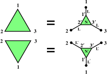
Figure 12: Graphical representation of (52).

Solving (53) for $\ell,n,F$, one obtains

$$\ell = \frac{C}{B},$$

$$n = \frac{(qB+C)^{3}}{AC^{2}-qB^{3}-3B^{2}C},$$

$$F = \frac{B^{3}(AC^{2}-qB^{2}-3B^{2}C)}{C^{2}(qB^{2}+C)^{3}},$$ (54)

and similarly one obtains $\ell^{\prime},n^{\prime},F^{\prime}$ in terms of $A^{\prime},B^{\prime},C^{\prime}$. The kagome-type lattice now becomes the one shown in Fig. 13(a).

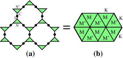
Figure 13: (a) The kagome-type lattice after transformation (52). (b) The lattice dual to (a).

The duality relation of Potts models with multi-site interactions has been formulated by Essam essam79 (see also wureview ). Following Essam, the dual to the lattice in Fig. 13(a) is the one shown in Fig. 13(b) with

$$e^{K} = (1+q/\ell)(1+q/\ell^{\prime}),$$

$$e^{M} = 1+q^{2}/n,$$

$$e^{M^{\prime}} = 1+q^{2}/n^{\prime}\,,$$ (55)

where the interaction $K$ is the dual to the two interactions $L$ and $L^{\prime}$ in series. We therefore are led to consider the Potts model on the triangular lattice shown in Fig. 13(b), where $M$ and $M^{\prime}$ are 3-site interactions.

For $M^{\prime}=0$, the partition function is $Z_{tri}(q;A,B,C)$ given by (2) with

$$W_{\bigtriangleup}(1,2,3)=e^{K(\delta_{12}+\delta_{23}+\delta_{31})}e^{M\delta_{123}},$$

or

$$A=1,\quad B=e^{K}-1,\quad C=e^{3K+M}-3e^{K}+2\,.$$ (56)

The exact critical frontier in this case is known. It is  $qA=C$, or

$$e^{3K+M}-3e^{K}+2=q.$$ (57)

For $M^{\prime}\not=0$ the critical frontier is not known. However, the critical frontier must be symmetric in $M$ and $M^{\prime}$. We now make a homogeneity assumption requiring $M$ and $M^{\prime}$ to appear homogeneously in the exponent of (57). The simplest way to do this is to extend (57) to

$$e^{3K+M+M^{\prime}}-3e^{K}+2=q\,.$$ (58)

The substitution of expressions of $K,M$ and $M^{\prime}$ in (55) and (54) into (57) now leads to (26).

IV Summary

We have considered the $q$-state Potts model and the related bond, site, and mixed site-bond percolation for triangular- and kagome-type lattices. For triangular-type lattices we obtained its exact critical frontier in the form of (9) without the usual assumption of a unique transition. We then applied the exact critical frontier in various applications. For kagome-type lattices we obtained a new critical frontier (26) by making use of a homogeneity assumption. We established that the new critical frontier is exact for $q=2$ and for site percolation on the kagome, martini, and other lattices. For the Potts and bond percolation models for which there is no exact solution, the new critical frontier gives numerical values of critical thresholds accurate to the order of $10^{-5}$. For mixed site-bond percolation, the homogeneity assumption gives rise to critical frontiers which are accurate when site occupation probabilities are $\sim 1$.

In summary, we emphasize that applications of the critical frontiers (9) and (26) are not limited to those reported in this paper. They can be extended to numerous other lattice models having a triangular or kagome symmetry, and thus they open the door to a host of previously unsolved problems.

References

- (1) R. B. Potts, Proc. Camb. Phil. Soc. 48, 106 (1952).
- (2) F. Y. Wu, Rev. Mod. Phys. 54, 235 (1982).
- (3) F. Y. Wu, J. Stat. Phys. 18, 115 (1978).
- (4) P. W. Kasteleyn and C. M. Fortuin, J. Phys. Soc. Japan (suppl.) 26, 11 (1969).
- (5) H. Kunz and F. Y. Wu, J. Phys. C 11 L1 (1978); Erratum, ibid. 11, L357 (1978).
- (6) D. Kim and R. J. Joseph, J. Phys. C 7, L167 (1974).
- (7) F. Y. Wu, J. Phys. C 12, L645 (1979).
- (8) F. Y. Wu, Phys. Rev. Lett 96, 090602 (2006).
- (9) D.-X. Yao, Y. L. Loh, E. W. Carlson and M. Ma, Phys. Rev. B 78, 024428 (2008).
- (10) Y. L. Loh, D.-X. Yao and E. W. Carlson, Phys. Rev. B 78, 224410 (2008).
- (11) R. M. Ziff and H. Gu, Phys. Rev. E 79 020102 (2009).
- (12) A. Haji-Akbari and R. M. Ziff, Phys. Rev. E 79, 021118 (2009).
- (13) R. J. Baxter, H. N. V. Temperley, and S. E. Ashley, Proc. R. Soc. London A 358, 535 (1978).
- (14) F. Y. Wu and K. Y. Lin, J. Phys. A 14, 629 (1980).
- (15) F. Y. Wu and R. K. P. Zia, J. Phys. A 14, 721 (1981).
- (16) C. Ding, Z. Fu, W. Guo and F. Y. Wu, Critical frontier of the Potts and percolation models on triangular-type and kagome-type lattices II: Numerical analysis, under preparation.
- (17) S. B. Kelland, Aust. J. Phys. 27, 813 (1974).
- (18) S. B. Kelland, J. Phys. A 7, 1907 (1974).
- (19) L. Chayes and H. K. Lei,J. Stat. Phys. 122, 647 (2006).
- (20) M. F. Sykes and J. W. Essam, J. Math. Phys. 5, 1117 (1964).
- (21) J. W. Essam, in Phase Transitions and Critical Phenomena, Vol. 2, Eds. C. Domb and M. S. Green (Academic, New York 1972).
- (22) J. W. Essam, J. Math. Phys 20, 1769 (1979).
- (23) P. N. Suding and R. M. Ziff, Phys. Rev. E 60, 275 (1999).
- (24) C. Chen, C. K. Hu and F. Y. Wu, J. Phys. A 31, 7855 (1998).
- (25) R. M. Ziff and P. N. Suding, J.Phys. A 30 5351 (1997).
- (26) C. R. Scullard and R. M. Ziff, Phys. Rev. E 73, 045102 (2006).
- (27) X. M. Feng, Y. J. Deng and H. W. J. Blöte, Phys. Rev. E 78 031136 (2008).
- (28) I. Syozi, in Phase Transitions and Critical Phenomena, Vol. 1, Eds. C. Domb and M. S. Green (Academic, New York 1972).
- (29) R. M. Ziff, private communication.
- (30) The corresponding expression, Eq. (4) in wuhu , for the critical frontier contains a typo missing a factor in the fourth term.
- (31) C. R. Scullard, Phys. Rev. E 73, 016107 (2006).
- (32) I. Kondor, J. Phys. C 13, L531 (1980).
- (33) R. M. Ziff, Phys. Rev. E 73, 016134 (2006).
- (34) T. Utiyama, Prog. Theor. Phys. 6, 907 (1951).
- (35) R. Parviainen, J. Phys. A 40, 9253 (2007).