Scattering from generalized Cantor fractals

Abstract

We consider a fractal with a variable fractal dimension, which is a generalization of the well known triadic Cantor set. In contrast with the usual Cantor set, the fractal dimension is controlled using a scaling factor, and can vary from zero to one in one dimension and from zero to three in three dimensions. The intensity profile of small-angle scattering from the generalized Cantor fractal in three dimensions is calculated. The system is generated by a set of iterative rules, each iteration corresponding to a certain fractal generation. Small-angle scattering is considered from monodispersive sets, which are randomly oriented and placed. The scattering intensities represent minima and maxima superimposed on a power law decay, with the exponent equal to the fractal dimension of the scatterer, but the minima and maxima are damped with increasing polydispersity of the fractal sets. It is shown that for a finite generation of the fractal, the exponent changes at sufficiently large wave vectors from the fractal dimension to four, the value given by the usual Porod law. It is shown that the number of particles of which the fractal is composed can be estimated from the value of the boundary between the fractal and Porod regions. The radius of gyration of the fractal is calculated analytically.

I Introduction

Small-angle scattering (SAS; X-rays, light, neutrons) Feigin and Svergun (1987); Zemb and Lindner (2002); Glatter and Kratky (1982) is one of the most important investigation techniques for the structural properties of fractal systems Pfeifer and Avnir (1983); Mandelbrot (1983); Pfeifer and Obert (1989); Peitgen et al. (2004) at the nanometer scale. This technique yields the Fourier transform of the spatial density distribution of a studied system within a wave vector range from $10^{-4}$ to $10^{-1}$Å^-1 and is thus very effective for object sizes from $10$ to $10^{4}$Å Feigin and Svergun (1987); Zemb and Lindner (2002); Glatter and Kratky (1982). Since only a finite range in wave vector space is available experimentally, the interpretation of the results requires theoretical models.

In the case of non-deterministic (random) fractals, different models for mass and surface fractals Bale and Schmidt (1984); Sinha et al. (1984); Martin and Ackerson (1985); Freltoft et al. (1986); Martin et al. (1986); Hurd et al. (1987) have been successfully developed and applied to a variety of materials Malcai et al. (1997). However, for deterministic fractals, only a few attempts have been made made Schmidt and Dacai (1986); Kjems and Schofield (1986); Schmidt (1991). This is probably due to the technological limitations encountered until just a few years ago in the preparation of fractal-like structures. Modern experimental techniques for obtaining deterministic fractal systems have now been developed Mayama and Tsujii (2006); Takeda et al. (2004); Cerofolini et al. (2008). Small-angle neutron scattering (SANS) from self-assembled porous silica materials Mayama and Tsujii (2006) was carried out by Yamaguchi et al. (2006) Yamaguchi et al. (2006). A molecular Sierpinski hexagonal gasket, the deterministic fractal polymer, was also obtained by chemical methods Newkome et al. (2006).

The main indicator of fractal structure is the power law behaviour of the scattering curve

$$I(q)\sim q^{-\alpha},$$ (1)

where $\alpha$ is the power law scattering exponent. $I$ is the diffracted intensity and $q=\frac{4\pi}{\lambda}\sin\theta$, where $2\theta$ is the scattering angle and $\lambda$ is the incident wavelength. The expnent $\alpha$ carries information regarding the fractal dimension of the scatterer Bale and Schmidt (1984); Sinha et al. (1984); Martin and Ackerson (1985); Freltoft et al. (1986); Martin et al. (1986); Hurd et al. (1987); Sorensen and Wang (1999): $\alpha=D$ for mass fractals and $\alpha=6-D$ for surface fractals. One can write down an even more general expression Pfeifer et al. (2002) for the exponent in a two-phase geometric configuration, where one phase is a mass fractal of fractal dimension $D_{\mathrm{m}}$ containing pores of fractal dimension $D_{\mathrm{p}}$. In addition, the boundary surface between the phases also forms a fractal of dimension $D_{\mathrm{s}}$. The exponent then reads $\alpha=2(D_{\mathrm{m}}+D_{\mathrm{p}})-D_{\mathrm{s}}-6$. In the particular case of a mass fractal, we have $D_{\mathrm{s}}=D_{\mathrm{m}}<3$ and $D_{\mathrm{p}}=3$, while for a surface fractal $D_{\mathrm{m}}=D_{\mathrm{p}}=3$ and $2<D_{\mathrm{s}}<3$.

The construction of non-random fractal models assumes the presence of an initial set (initiator) and a generator (iterative operation). Usually, an initiator is divided into subparts. Some of them are then removed according to an iterative rule and the process is repeated for each remaining part.

In contrast with the simple power law behaviour above [equation (1)], the scattering from non-random fractals, such as the Menger sponge, fractal jack Schmidt and Dacai (1986) or other surface-like type Schmidt (1991), shows a successive superposition of maxima and minima decaying as a power law, which can be called a generalized power law. This is due to spatial order in non-random fractals: the scattering curve $I(q)$, being the Fourier transform of the pair distribution function, oscillates by reason of singularities in this function or its derivatives. If there is disorder in the system then the singularities are smeared out, as in the case of random fractals, the behaviour of which follows the power law of equation (1). On the other hand, real physical systems always exhibit a specific kind of disorder, polydispersity. Below, we show that when the polydispersity of non-random fractals is taken into account, these local oscillations cancel out with increasing width of the distribution function. This is consistent with the results obtained for a similar fractal, the Menger sponge, by averaging over a Schulz distribution function Schmidt (1995).

The existing models Schmidt and Dacai (1986); Schmidt (1991) assume a given fractal dimension, which imposes some restrictions on applying the models to real systems. In this paper, a generalization of Cantor sets is considered that allows us to control the fractal dimension using a scaling factor. The scattering intensity of randomly oriented generalized Cantor sets is obtained analytically for mono- and polydisperse systems. Our method is based on the approach that was successfully employed in some aspects for other similar systems of non-random fractals such as the Menger sponge Schmidt and Dacai (1986).

Numerous examples of the fractal-like behaviour were obtained experimentally in collaboration with one of the authors of this paper (AIK) for different kind of objects, namely soils Fedotov et al. (2006); Fedotov et al. (2007a, b), biological objects Lebedev et al. (2008) and nanocomposites Dokukin et al. (2007). Only three parameters are extracted from the fractal scattering intensity: its exponent $\alpha$ [see equation (1)], and the edges of the fractal region in $q$-space, which appear as ”knees” in the scattering line on a logarithmic scale. Other parameters are not usually obtained from small-angle neutron scattering (SANS) curves.

If some features of the fractal structure are available from other considerations, one can construct a model and obtain additional information on the fractal parameters. Note that a real physical system does not possess an infinite scaling effect and the number of iterations is always finite. In this paper we calculate the scattering from generalized Cantor sets for a finite number of iterations. As discussed below, many features of the scattering are quite general; in particular, one can estimate the number of particles from which the fractal is formed.

II Construction of the generalized Cantor set

The well known Cantor set is created by repeatedly deleting the open central third of a set of line segments. One can construct various generalizations of the set by, say, cutting the segments into a different number of intervals or choosing another scaling factor (see, e.g. Gouyet (1996)). Below, we explicitly describe a three-dimensional generalization of the Cantor set, which is used for studying the scattering in the subsequent sections.

The generalized Cantor set in three dimensions can be constructed from a homogeneous cube by iterations, which we will call approximants. The zero-order iteration (initiator) is the cube itself with side length $l_{0}$, which can be specified in Cartesian coordinates as a set of points obeying the conditions $-l_{0}/2\leqslant x\leqslant l_{0}/2$, $-l_{0}/2\leqslant y\leqslant l_{0}/2$, $-l_{0}/2\leqslant z\leqslant l_{0}/2$. The first iteration removes all points from the cube with coordinates $-\gamma l_{0}/2<x<\gamma l_{0}/2$ or $-\gamma l_{0}/2<y<\gamma l_{0}/2$ or $-\gamma l_{0}/2<z<\gamma l_{0}/2$. The dimensionless scaling factor $\gamma$ can take any value between zero and three. Thus, the initial cube is divided into 27 parts, the eight cubes are left in the corners, with edge length $(1-\gamma)l_{0}/2$, and the 19 parallelepipeds are removed (see Fig. 1, upper panel).

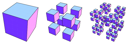
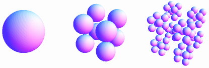
Figure 1: Zero, first and second iterations (approximants) for the generalized Cantor set, composed of cubes (upper panel) and balls (lower panel).

In order to obtain the second approximant, one should do the same with each of the eight cubes, thus leaving 64 cubes of side length $(1-\gamma)^{2}l_{0}/4$. It is not difficult to see that the $m$th approximant to the three-dimensional Cantor set is composed of $N_{m}=8^{m}$ cubes of the side length

$$l_{m}=(1-\gamma)^{m}l_{0}/2^{m}.$$ (2)

The generalized Cantor set is obtained in the limit $m\to\infty$.

The Hausdorff dimension Mandelbrot (1983) of the set can be determined from the intuitively apparent relation $N_{m}\sim(l_{0}/l_{m})^{D}$ for a large number of iterations, which yields

$$D=\lim_{m\to\infty}\frac{\ln N_{m}}{\ln(l_{0}/l_{m})}=-\frac{3\ln 2}{\ln\beta_{\mathrm{s}}},$$ (3)

where the scaling factor $0<\beta_{\mathrm{s}}<1$ for each iteration is defined as

$$\beta_{\mathrm{s}}\equiv(1-\gamma)/2.$$ (4)

In the same manner, it can be shown that the fractal dimension of the surface coincides with that of the bulk structure. We then have a mass fractal, the dimension of which can be varied between zero and three by changing the parameter $\gamma$.

Note that the generalized Cantor set composed of cubes is simply the direct product of three one-dimensional generalized Cantor sets (Fig. 2). This means that the point $\bm{r}=(x,y,z)$ belongs to the three-dimensional set if and only if each of the coordinates $x$, $y$ and $z$ belongs to the one-dimensional set. The fractal (Hausdorff) dimension of the one-dimensional generalized Cantor set is three times smaller than that of the three-dimensional set [equation (3)].

Figure 2: The first five iterations for the one-dimensional generalized Cantor set with scaling factors $\gamma=0.2$ (left) and $\gamma=0.5$ (right). It is generated by removing at the $m$th iteration the central interval of length $\gamma^{m}l_{0}$ from each remaining segment. The fractal (Hausdorff) dimension of the one-dimensional generalized Cantor set is equal to $-\ln 2/\ln\beta_{\mathrm{s}}$, where $\beta_{\mathrm{s}}$ is given by equation (4). At $\gamma=1/3$ we obtain the usual Cantor set with fractal dimension $\ln 2/\ln 3=0.6309\ldots$.

One can generalize the fractal construction, replacing the cubes with any solid three-dimensional shape and using the same scaling [equation (4)] for each iteration. For example, a ball of arbitrary radius $R\leqslant l_{0}/2$ in the center of the cell can be used as an initiator instead of the initial cube (Fig. 1, lower panel). One can see that the fractal dimension is still given by [equation (3)].

III Form factor of the monodisperse set

III.1 General remarks

We consider a two-phase system of particles, consisting of small pieces of “mass”. The masses are embedded in a solid matrix, which can be associated with the “pores” discussed in Sec. I. The particles are also immersed in the solid matrix or dissolved in a solution of the same scattering length density as pores. The scattering length densities are $\rho_{\mathrm{m}}$ for the mass and $\rho_{\mathrm{p}}$ for the pores. They are determined by the relation $\rho\equiv\sum_{i}b_{i}/\Delta V$, where the summation is over the scattering centers located in the volume $\Delta V$. The difference $\rho_{\mathrm{m}}-\rho_{\mathrm{p}}$ is called the scattering contrast. In what follows, we mean by particle the $m$th approximant to the generalized Cantor set.

The neutron scattering cross section per unit volume of a sample is given in Feigin and Svergun (1987) as

$$\frac{1}{V^{\prime}}\frac{d\sigma}{d\Omega}=n(\rho_{\mathrm{m}}-\rho_{\mathrm{p}})^{2}V^{2}\langle|F(\bm{q})|^{2}\rangle,$$ (5)

where $\bm{q}$ is momentum transfer, $n$ is the number of particles per unit volume and $V$ is the total volume of the mass in the particle. [Note that, in the literature, the quantity $VF(\bm{q})$ is sometimes called the scattering amplitude, while the squared and averaged quantity $V^{2}\langle|F(\bm{q})|^{2}\rangle$ is what is meant by form factor.] The normalized scattering form factor is defined as

$$F(\bm{q})\equiv\frac{1}{V}\int_{V}e^{-i\bm{q}\cdot\bm{r}}d\bm{r},$$ (6)

and the symbol $\langle\ldots\rangle$ denotes the mean value over all orientations of the particle. Here we assume that the particles are randomly oriented in space and their positions are not correlated. The latter means that we neglect particle interactions and put the interparticle structure factor equal to 1, which is quite reasonable if the average distance between the particles is sufficiently large.

If the probability of any orientation is the same, then the mean value can be calculated by averaging over all directions $\bm{n}$ of the momentum transfer $\bm{q}=q\bm{n}$, that is, by integrating over the solid angle in the spherical coordinates ${q}_{x}=q\cos\varphi\sin\vartheta$, ${q}_{y}=q\sin\varphi\sin\vartheta$ and ${q}_{z}=q\cos\vartheta$

$$\langle f(q_{x},q_{y},q_{z})\rangle\equiv\frac{1}{4\pi}\int_{0}^{\pi}d\vartheta\sin\vartheta\int_{0}^{2\pi}d\varphi\,f(q,\vartheta,\varphi).$$ (7)

Once we know the absolute values of the intensity [equation (5)], the concentration of fractals and the contrast, we can obtain the fractal volume from the scattering at zero momentum.

III.2 An analytical formula for the fractal form factor

One can easily obtain an explicit analytical formula for the form factor [equation (6)] of the $m$th approximant. A similar method for obtaining the form factor of non-random fractals was used in Schmidt and Dacai (1986) (see also a generalization in Hamburger-Lidar (1996)). The zeroth approximant is an initiator with a form factor $F_{0}(\bm{q})$. If the initiator is a cube of edge $l_{0}$ we have $F_{0}=F_{\mathrm{c}}$, where

$$F_{\mathrm{c}}(\bm{q})=\frac{\sin(q_{x}l_{0}/2)}{q_{x}l_{0}/2}\frac{\sin(q_{y}l_{0}/2)}{q_{y}l_{0}/2}\frac{\sin(q_{z}l_{0}/2)}{q_{z}l_{0}/2}.$$ (8)

In the case of the ball of radius $R$, we have $F_{0}=F_{\mathrm{b}}$ with

$$F_{\mathrm{b}}(\bm{q})=3\frac{\sin(qR)-qR\cos(qR)}{(qR)^{3}},\quad q=|\bm{q}|.$$ (9)

To obtain the first-order formula, one can use three simple properties of the the scattering form factor [equation (6)] for a particle of arbitrary shape:
i) If we scale the entire length of a particle as $l\to\beta l$, then $F(\bm{q})\to F(\beta\bm{q})$.
ii) If a particle is translated $\bm{r}\to\bm{r}+\bm{a}$, then $F(\bm{q})\to F(\bm{q})\exp(-i\bm{q}\cdot\bm{a})$.
iii) If a particle consists of two non-overlapping subsets $\mathrm{I}$ and $\mathrm{II}$, then $F(\bm{q})=\big{(}V_{I}F_{I}(\bm{q})+V_{\mathrm{II}}F_{\mathrm{II}}(\bm{q})\big{)}/(V_{\mathrm{I}}+V_{\mathrm{II}})$.

The first approximant consists of eight cubes (balls), which differ from the initial cube by the scaling factor of equation (4) and the center positions of which are shifted from the center of the initial cube by the vectors $\bm{a}_{j}=\{\pm\beta_{\mathrm{t}}l_{0},\pm\beta_{\mathrm{t}}l_{0},\pm\beta_{\mathrm{t}}l_{0}\}$ with various combinations of the signs. Here we put by definition

$$\beta_{\mathrm{t}}\equiv(1+\gamma)/4.$$ (10)

Using the definitionof equation (6) and the properties i), ii) and iii), we obtain

$$V_{1}F_{1}(\bm{q})=\sum_{j=1}^{8}\beta_{\mathrm{s}}^{3}V_{0}F_{0}(\beta_{\mathrm{s}}\bm{q})\exp(-i\bm{q}\cdot\bm{a}_{j}).$$ (11)

Here, the total volume of the first approximant is given by $V_{1}=8V_{0}\beta_{\mathrm{s}}^{3}$, and $V_{0}$ is the volume of the initial cube (ball). Writing down the sum explicitly yields

$$F_{1}(\bm{q})=G_{1}(\bm{q})F_{0}(\beta_{\mathrm{s}}\bm{q}),$$ (12)

where we introduce the function $G$ defined as

$$G_{1}(\bm{q})\equiv\cos(q_{x}l_{0}\beta_{\mathrm{t}})\cos(q_{y}l_{0}\beta_{\mathrm{t}})\cos(q_{z}l_{0}\beta_{\mathrm{t}}).$$ (13)

For the second approximant we repeat the same operation on $F_{1}(\bm{q})$ and obtain

$$F_{2}(\bm{q})=G_{1}(\bm{q})F_{1}(\beta_{\mathrm{s}}\bm{q})=G_{1}(\bm{q})G_{1}(\beta_{\mathrm{s}}\bm{q})F_{0}(\beta_{\mathrm{s}}^{2}\bm{q}).$$ (14)

In the same manner, we infer the general relation

$$F_{m}(\bm{q})=P_{m}(\bm{q})F_{0}(\beta_{\mathrm{s}}^{m}\bm{q}),$$ (15)

where

$$P_{m}(\bm{q})\equiv G_{1}(\bm{q})G_{2}(\bm{q})\ldots G_{m}(\bm{q}),$$ (16)

and

$$G_{m}(\bm{q})\equiv\cos(q_{x}l_{0}\beta_{\mathrm{t}}\beta^{m-1}_{\mathrm{s}})\cos(q_{y}l_{0}\beta_{\mathrm{t}}\beta^{m-1}_{\mathrm{s}})\cos(q_{z}l_{0}\beta_{\mathrm{t}}\beta^{m-1}_{\mathrm{s}})$$ (17)

for $m=1,2,\ldots$. We can also put, by definition, $G_{0}(\bm{q})=1$ and $P_{0}(\bm{q})=1$ in order to describe the initiator.

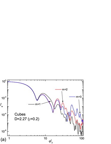
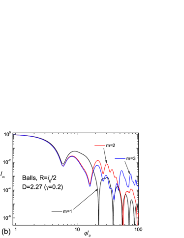
Figure 3: Scattering intensities [equation (18)] for the first three iterations of the generalized Cantor set composed of (a) cubes and (b) balls. The radius of the initial ball (initiator) is $R=l_{0}/2$. The intensities can be estimated as a product [equation (19)] of the fractal structure factor and scaled zero iteration, shown in Fig. 4.

To obtain the cross section given by equation (5), we should calculate the mean value of $|F_{m}(\bm{q})|^{2}$ over all directions $\bm{n}$ of the momentum transfer using equation (7)

$$I_{m}(ql_{0})\equiv\langle|F_{m}(\bm{q})|^{2}\rangle,$$ (18)

where $m=0,1,\ldots$. Here, the form factor $F_{m}(\bm{q})$ is given by equations (15)-(17) in conjunction with equations (4) and (10); the initial form factor $F_{0}$ is represented by equation (8) or (9). Note that the intensity equation (18) of the $m$th monodisperse appoximant depends on the wave vector and the initial length through the product $ql_{0}$ only. The results for the first three iterations are shown in Fig. 3.

III.3 Discussion of results

These results are in accordance with scattering from similar systems like the Menger sponge, displaying the same behaviour of the scattering curve Schmidt and Dacai (1986). Those authors first omitted the last multiplier in equation (15), assuming that $ql_{0}\beta_{\mathrm{s}}^{m}\ll 1$, and then used the expansion of cosines that allows for reducing the intensity formula to a sum of quite simple terms. However, the number of terms grows exponentially on increasing the number of iterations, and the method becomes very time-consuming even for $m=4$. By contrast, using the straightforward integration in equation (18), we can employ the exact relation [equation (15)] for arbitrary $m$, which can yield a substantial improvment in accuracy. At sufficiently large $ql_{0}$, the main contribution to the integral comes from a small number of narrow and high spikes, which is typical for an interference pattern. Nevertheless, the integral can be evaluated even at sufficiently large values of $ql_{0}$, up to $10^{4}$ in a reasonable amount of time.

III.3.1 The fractal structure factor

The scattering intensity can be approximately represented as

$$I_{m}(ql_{0})\simeq S_{m}(q)\,\langle|F_{0}(\beta_{\mathrm{s}}^{m}\bm{q})|^{2}\rangle/N_{m},$$ (19)

where

$$S_{m}(q)\equiv N_{m}\langle|P_{m}(\bm{q})|^{2}\rangle.$$ (20)

Here, $N_{m}=8^{m}$ is the total number of cubes (balls) in the $m$th iteration, and the quantity $S_{m}(q)$ is the fractal structure factor (see, e.g. March et al. (1967)). The latter is $N_{m}$ times larger than the intensity given by equation (18) with $F_{0}=1$, for instance when the radius of the ball tends to zero. The form factor of the ball [equation (9)] is isotropic, and hence relation (19) is satisfied exactly. The structure factor carries information about the relative positions of the cubes (balls) in the fractal. Indeed, using the definition (6) and the analytical formula for the form factor [equation (15)], one can obtain

$$P_{m}(\bm{q})=\frac{1}{N_{m}}\sum_{1\leqslant j\leqslant N_{m}}\exp[-i\bm{r}_{j}^{(m)}\cdot\bm{q}],$$ (21)

where $\bm{r}_{j}^{(m)}$ are the center-of-mass coordinates of cubes (balls). Then the fractal structure factor [equation (20)] reads

$$S_{m}(q)=1+\frac{2}{N_{m}}\sum_{1\leqslant k<j\leqslant N_{m}}\!\!\dfrac{\sin qr^{(m)}_{jk}}{qr^{(m)}_{jk}},$$ (22)

where

$$r^{(m)}_{jk}\equiv\big{|}\bm{r}_{j}^{(m)}-\bm{r}_{k}^{(m)}\big{|}.$$ (23)

Deriving this last relation, we use the formula $\langle\exp(i\bm{a}\cdot\bm{q})\rangle=\sin(aq)/(aq)$, which follows from equation (7).

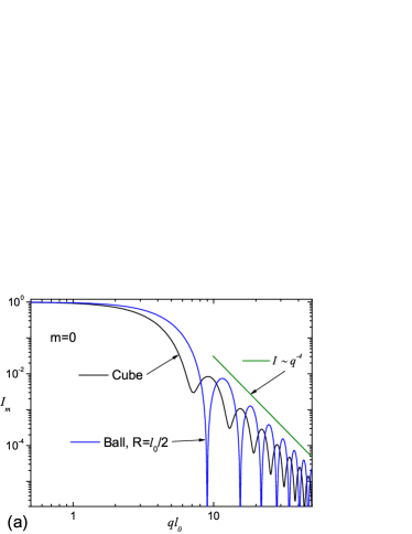
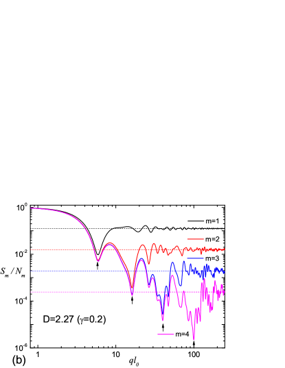
Figure 4: Scattering intensities [equation (18)] for various system geometries. (a) Zero iteration: intensities for a cube of edge $l_{0}$ and a ball of radius $R=l_{0}/2$. The positions of the maxima obey Porod‘s law. (b) The structure factor of the generalized Cantor fractal [equation (20)] in units of $N_{m}$, where $N_{m}=8^{m}$ is the total number of cubes (balls) in the $m$th iteration. The diagram represents the first four iterations at $\gamma=0.2$, which corresponds to the fractal dimension $D\simeq 2.27$. The asymptote for the structure factor equals 1 when $ql_{0}\gtrsim 1/\beta^{m}_{\mathrm{s}}$ (see text). The deep minima marked by vertical arrows can be estimated using equation (26).

At zero momentum, relation (22) reads $S_{m}(0)=N_{m}$. At sufficiently large momentum, equation (22) yields the asymptotic relation

$$S_{m}(q)\simeq 1.$$ (24)

The underlying physics is quite clear: when the reciprocal wave vector is much smaller than the characteristic variance of the distance between the points then the scattering pattern does not “feel” their spatial correlations. The characteristic variance is of the order $ql_{0}\beta_{\mathrm{t}}\beta^{m}_{\mathrm{s}}\sim ql_{0}\beta^{m}_{\mathrm{s}}$, and the asymptote is attained when

$$ql_{0}\gg 1/\beta_{\mathrm{s}}^{m}.$$ (25)

The structure factor reaches its deepest minima (see Fig. 4b) when most of the objects inside the fractal interfere out of phase. This happens when the most common distance between the center of mass of the objects equals $\pi/q$. Taking the value of the distance $2l_{0}\beta_{\mathrm{t}}\beta^{k-1}_{\mathrm{s}}$ (see Sec. II), we obtain an estimation of the minima positions for the $m$th iteration

$$q_{k}l_{0}\simeq\frac{\pi}{2\beta_{\mathrm{t}}\beta^{k-1}_{\mathrm{s}}},\quad k=1,\ldots,m.$$ (26)

One can see that the structure factor has as many minima as the number of iterations.

III.3.2 Generalized power law

As was noted in Sec. I, rigid spatial correlations between points in a non-random fractal yield singularities in the form of $\delta$-functions, which leads to oscillations in the structure factor (Fig. 4b). The weight of each $\delta$-functions follows the power law with respect to the distance between points $r^{(m)}_{jk}$, as determined by the fractal dimension. As a consequence, the scattering curve shows groups of maxima and minima which are superimposed on a monotonically decreasing curve proportional to some power of the absolute value of the scattering vector (generalized power law). Short-range correlations govern the long-range wave vector oscillations and vice versa. It is essential that the oscillations are not damped on increasing the number of iterations, because this influences only the short-range correlations and hence the scattering behaviour at large momentum.

An advantage of the model considered here is the explicit analytical expressions (15)-(17), which allow us to estimate easily the fractal region where the generalized power law aplies. If the cosine argument in $G_{m+1}$ is much smaller than 1, then a further increasing in $m$ does not lead to an essential correction and the $m$th iteration reproduces the intensity that the ideal Cantor fractal would give at this argument. Thus, the $m$th iteration works well within the region $ql_{0}\beta^{m}_{\mathrm{s}}\ll 1$, where we use the estimation $\beta_{\mathrm{t}}\sim 1$. Such behaviour can be seen in Fig. 3.

On the other hand, within the Gunier region $ql_{0}\lesssim 1$ the intensity is very close to 1 and we have a plateau in the logarithmic scale. The generalized power-law behaviour is then observed in the region

$$1\ll ql_{0}\ll 1/\beta^{m}_{\mathrm{s}}.$$ (27)

This estimation indicates two typical length scales important for a fractal, its size $l_{0}$ and the characteristic distance inside the $m$th iteration $l_{0}\beta^{m}_{\mathrm{s}}$ Schmidt (1991). In the fractal region $F_{0}(\beta^{m}_{\mathrm{s}}\bm{q})\simeq 1$, and we obtain from equation (19)

$$I_{m}(ql_{0})\simeq S_{m}(q)/8^{m}.$$ (28)

Beyond the fractal region, when the inequality of equation (25) is satisfied, we derive from equations (19) and (24)

$$I_{m}(ql_{0})\simeq\langle|F_{0}(\beta_{\mathrm{s}}^{m}\bm{q})|^{2}\rangle/8^{m}.$$ (29)

It follows that, beyond the fractal region, the scattering intensity resembles the intensity of the initiator, i.e. a cube or ball in the present case (Fig. 5). In particular, the maxima of the curve obey Porod’s law Glatter and Kratky (1982).

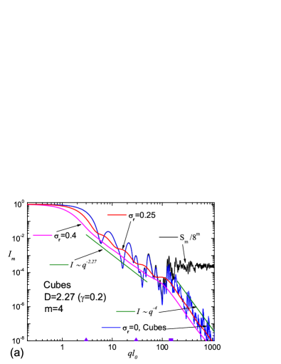
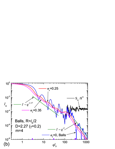
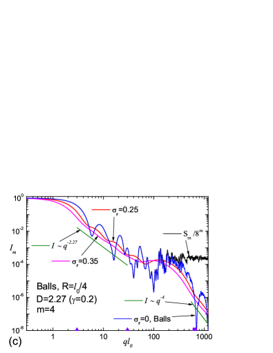
Figure 5: Influence of polydispersity on scattering from Cantor fractals of (a) cubes and (b) and (c) balls. The radius of the initial ball (initiator) is $R=l_{0}/2$ in part (b) and $R=l_{0}/4$ in part (c). The upper monodispersive curve is the structure factor [equation (20)], which in the fractal region [equation (27)] is proportional to the exact intensity [equation (28)]. The borders of the fractal region are shown with filled (violet) triangles on the horizontal axes. In this region, the exponent of the polydisperse curve equals the fractal dimension, while at large momentum $qR\gg 1/\beta_{\mathrm{s}}^{m}$, the power law exponent changes from the fractal exponent to four, given by the usual Porod law. The beginning of the Porod region is shown by the filled (violet) squares.

III.3.3 The radius of gyration

One can calculate the radius of gyration $R_{\mathrm{g}}$ of the fractal. By definition Feigin and Svergun (1987), in the Guinier region $I(q)=I(0)(1-q^{2}R_{\mathrm{g}}^{2}/3+\ldots)$. Expanding equation (15) in a power series in $q$ and substituting the result into equation (18) yield

$$R_{\mathrm{g}}=\sqrt{\beta_{\mathrm{s}}^{2m}R_{\mathrm{g}0}^{2}+3\beta_{\mathrm{t}}^{2}\frac{1-\beta_{\mathrm{s}}^{2m}}{1-\beta_{\mathrm{s}}^{2}}l_{0}^{2}},$$ (30)

where $R_{\mathrm{g}0}=l_{0}/2$ for a uniform cube and $R_{\mathrm{g}0}=R\sqrt{3/5}$ for a uniform ball. The limit $m\to\infty$ gives the radius of gyration of the ideal Cantor fractal

$$R_{\mathrm{g}}=\frac{\sqrt{3}\beta_{\mathrm{t}}l_{0}}{\sqrt{1-\beta_{\mathrm{s}}^{2}}}.$$ (31)

As expected, the characteristics of the ideal fractal do not depend on specific shapes from which the fractal is constructed.

IV Form factor of polydisperse sets

Here we study a specific kind of polydispersity, when the whole fractal is proportionally scaled and the scales are distributed. This implies that it is sufficient to consider the distribution of the fractal length in the above formulae. Then the distribution function $D_{N}(l)$ of the scatterer sizes can be considered in such a way that $D_{N}(l)dl$ gives the probability of finding a fractal whose size falls within the interval $(l,l+dl)$. The intensity can then be written as

$$I_{m}^{\rm poly}(q)=\frac{\int_{0}^{\infty}\langle F_{m}^{2}(\bm{q})\rangle V_{m}^{2}(l)D_{N}(l)\,dl}{\int_{0}^{\infty}V_{m}^{2}(l)D_{N}(l)\,dl},$$ (32)

where $V_{m}$ is the total volume of the $m$th approximant,

$$V_{m}=l^{3}(2\beta_{\rm s})^{3m}.$$ (33)

The influence of particle size distribution on the intensity scattering curves is essentially determined by its breadth. Narrow distributions (i.e. log-normal, Schulz, Gauss) have no influence on the scattering exponent but control a smoothing of the intensity curve, reproducing the power law behaviour for a certain value of the variance, while broad ones can change even the scattering exponent Martin et al. (1986).

In order to study this influence on scattering from the Cantor sets, we consider a log-normal distribution given by

$$D_{N}(l) =\frac{1}{\sigma l\sqrt{2\pi}}\exp\left[-\frac{\big{(}\ln(l/l_{0})+\sigma^{2}/2\big{)}^{2}}{2\sigma^{2}}\right],$$ (34)

$$\sigma \equiv\sqrt{\ln(1+\sigma^{2}_{\mathrm{r}})}.$$

Here, $l_{0}$ and $\sigma_{\mathrm{r}}$ are the mean length and its relative variance, respectively, i.e.

$$l_{0}\equiv\langle l\rangle_{D},\quad\sigma_{\mathrm{r}}\equiv\sqrt{\langle l^{2}\rangle_{D}-l_{0}^{2}}/l_{0},$$ (35)

where $\langle\ldots\rangle_{D}\equiv\int_{0}^{\infty}\ldots D_{N}(l)\,dl$. One can see that the relative variance regulates the width of the distribution.

Fig. 5 represents the scattering curves from mono- and polydisperse Cantor sets for the fourth iteration at $\gamma=0.2$. The curves corresponding to the polydisperse cases approach the monodisperse ones as the distribution width $\sigma_{\mathrm{r}}$ tends to zero. Smoothing of intensity curve [equation (32)] increases when the width of the distribution $\sigma_{\mathrm{r}}$ becomes larger. The most interesting effect is changing the power law exponent from the fractal dimension $D$ in the fractal region [equation (27)] to the usual Porod exponent of four beyond this region. Here the intensity is approximately proportional to the scaled intensity of the initiator, according to equation (29), thus giving Porod’s law.

One can see the well in the intermediate region $ql_{0}\sim 1/\beta_{\mathrm{s}}^{m}$, where the monodisperse curve is shifted up to the asymptote $1/8^{m}$. The well becomes even more pronounced when the size of the initiator becomes smaller, compare Fig. 5(b) and (c). For a very small initiator size, a plateau should appear here. The reason is that the border of the Porod region shifts forward, and until it reaches this border the intensity profile coincides with the smoothed structure factor, which has an “infinite” plateau. Such behaviour of the scattering intensity has been observed experimentally Lebedev et al. (2008). A phenomenological approach has been developed by Beaucage (1995) Beaucage (1995) for studying various exponents in the scattering intensity.

Note that the appearance of the well or “shelf” between the fractal and Porod regions near the volume $1/N_{m}$ is a consequence of the general asymptote 1 of the fractal structure factor [equation (24)]. Thus, the position of the “shelf” allows us to estimate the volume of particles that form the fractal, provided the total fractal volume is known (see discussion in Sec. III.1).

Expanding equation (32) in a power series in $q$ and integrating over the distribution, we arrive at the radius of gyration given by equations (30) or (31) multiplied by the factor $(1+\sigma^{2}_{\mathrm{r}})^{13/2}$.

V Conclusions

We consider a model that generalizes the well known one-dimensional Cantor set. It is characterized by a scaling factor controlling the fractal dimension, which can be varied from zero to three. This is beyond the standard for mass fractals from an experimental point of view Malcai et al. (1997), since fractal dimensions less than 1 have not yet been observed. The form factor of the generalized Cantor set is calculated analytically for arbitrary iteration. This allows us to evaluate the scattering intensity for mono- and polydisperse fractals by means of simple integrals. We find the values of the asymptotes of the fractal structure factor and reveal their nature. The radius of gyration is obtained analytically as well.

The suggested model describes changing the power law exponent from the fractal dimension to the usual Porod exponent beyond the fractal region. In the intermediate region a typical well or “shelf” arises, which can be observed experimentally Lebedev et al. (2008). In comparison with Schmidt and Dacai (1986) Schmidt and Dacai (1986), we not only calculate the scattering intensity for large momenta but also explain its behaviour. Moreover, if an experiment observes the threshold between the fractal and Porod regions, the approach suggested here yields the number of particles in the fractal set. Another way to describe the experimental data for fractals is ab initio methods, see e.g. Ozerin et al. (2006).

In a number of cases we have a priori information about the fractal structure, for instance when the fractal synthesis is well controlled by chemical methods. One can then build a fractal model with many parameters and use this model to obtain additional information from the scattering data. The generalized Cantor set is an example of such a construction. A similar scheme can be developed by the same method for other types of fractal sets.

The model can be extended to match specific needs in various ways, including different values of the scaling factor at each iteration, and different probability distributions for the fractal length and the shapes from which it is constructed.