Spectra and Systems of Equations

Abstract.

In a previous work we introduced an elementary method to analyze the periodicity of a generating function defined by a single equation $y=G(x,y)$. This was based on deriving a single set-equation $Y={\Gamma}(Y)$ defining the spectrum of the generating function. This paper focuses on extending the analysis of periodicity to generating functions defined by a system of equations ${\bf y}={\bf G}(x,{\bf y})$.

The final section looks at periodicity results for the spectra of monadic second-order classes whose spectrum is determined by an equational specification—an observation of Compton shows that monadic-second order classes of trees have this property. This section concludes with a substantial simplification of the proofs in the 2003 foundational paper on spectra by Gurevich and Shelah [16], namely new proofs are given of: (1) every monadic second-order class of $m$-colored functional digraphs is eventually periodic, and (2) the monadic second-order theory of finite trees is decidable.

1. Introduction

Following Flajolet and Sedgewick [15], a combinatorial class ${\mathcal{A}}$ is a class of objects with a function $||\ ||$ that assigns a positive integer size to each object in the class, satisfying the condition that there are only finitely many objects of each size. We deviate from the definition in [15] by not having objects of size 0. Letting $a(n)$ be the number of objects of size $n$, one has the generating function $\displaystyle A(x)=\sum_{n=1}^{\infty}a(n)x^{n}$.

1.1. Generating Functions defined by Systems of Equations

Cayley [7] noted in his very first paper on trees in 1857 that one has an equation

$$\sum_{n\geq 1}a(n)x^{n}\ =\ x\cdot\prod_{n\geq 1}(1-x^{n})^{-a(n)}$$

which yields a recursive procedure to calculate the values of $a(n)$. Cayley used this to calculate the first 13 coefficients $a(n)$, that is, the numbers of such trees of sizes 1 through 13 (two of the numbers were not calculated correctly). In 1937 Pólya (see [18]) would rewrite this equation as

$$A(x)\ =\ x\cdot\exp\left(\sum_{m=1}^{\infty}A(x^{m})/m\right),$$

a form which could be viewed as a functional equation for $A(x)$, with important analytic properties based on the fact that the radius of convergence $\rho$ of $A(x)$ is less than 1 (which is easily proved). This allowed Pólya to invoke the implicit function theorem and results of Darboux to show that $A(x)$ has a square-root singularity at $\rho$, leading to the asymptotic form $C\rho^{-n}n^{-3/2}$ for the coefficients $a(n)$. Many natural classes of trees are specified recursively by a single equation, for example planar binary trees, also known as $(0,2)$-trees, where the generating function $A(x)$ solves the equation $y\ =\ x\big{(}1+y^{2}\big{)}$.

Although generating functions defined by a single equation cover many interesting cases, Example 33, at the end of the introduction section, hints at the value of considering generating functions defined by a system of several equations.

1.2. Spectra and Periodicity

In 1952 the Journal of Symbolic Logic initiated a section devoted to unsolved problems in the field of symbolic logic. The first problem, posed by Heinrich Scholz [20], was the following. Given a sentence $\varphi$ from first-order logic, he defined the spectrum of $\varphi$ to be the set of sizes of the finite models of $\varphi$. For example, binary trees can be defined by such a $\varphi$, and its spectrum is the arithmetical progression $\{1,3,5,\ldots\}$. The algebraic structures called fields can also be defined by such a $\varphi$, with the spectrum being the set $\{2,4,\ldots,3,9,\ldots\}$ of powers of prime numbers. The possibilities for the spectrum of a first-order sentence are amazingly complex.

Scholz’s problem was to find a necessary and sufficient condition for a set $S$ of natural numbers to be the spectrum of some first-order sentence $\varphi$. This problem led to a great deal of research by logicians on the topic of spectra — see for example the recent survey paper [13] of Durand, Jones, Makowsky, and More. Periodicity is one of the properties that has been examined in the context of studying spectra.

Definition 1.

${\mathbb{N}}$ is the set of non-negative integers, ${\mathbb{P}}$ is the set of positive integers.

For $A\subseteq\mathbb{N}$,

• $A$ is periodic if there is a positive integer $p$ such that $p+A\subseteq A$, that is, $a\in A$ implies $p+a\in A$. Such an integer $p$ is a period of $A$.

• A is eventually periodic if there is a positive integer $p$ such that $p+A$ is eventually in $A$, that is, there is an $m$ such that for $a\in A$, if $a\geq m$ then $p+a\in A$. Such a $p$ is an eventual period of $A$.

Clearly every arithmetical progression and every cofinite subset of ${\mathbb{N}}$ is periodic; and every periodic set is eventually periodic. Finite sets are eventually periodic. As will be seen, periodicity seems to be a natural property for the spectra of combinatorial classes specified by a system of equations. The famous Skolem-Mahler-Leech Theorem (see, for example, [15], p. 266) says that the spectrum of every rational function $P(x)/Q(x)$ in $\mathbb{Q}(x)$ is eventually periodic. Consequently polynomial systems ${\bf y}={\bf G}(x,{\bf y})$ with rational coefficients that are linear in the variables $y_{i}$, and with a non-singular Jacobian matrix $\partial({\bf y}-{\bf G})/\partial{\bf y}$, have power series solutions $y_{i}=T_{i}(x)$ such that the support sets of the coefficient sequences $t_{i}(n)$ of the $T_{i}(x)$ are eventually periodic. However, much simpler methods give this periodicity result for the non-negative ${\bf y}$-linear systems considered in this paper.

If the spectrum $A$ of a combinatorial class ${\mathcal{A}}$ is eventually periodic then one has the possibility, as in the case of regular languages and well-behaved irreducible systems, that the class ${\mathcal{A}}$ decomposes into a finite subclass ${\mathcal{A}}_{0}$, along with finitely many subclasses ${\mathcal{A}}_{i}$, such that the spectrums $A_{i}$ are arithmetical progressions $a_{i}+b_{i}\cdot{\mathbb{N}}$, and the generating functions $A_{i}(x)$ have well-behaved coefficients (e.g., monotone increasing) on $A_{i}$.

In the study of spectra of combinatorial classes, logicians have dominated the literature thanks to powerful tools like Ehrenfeucht-Fraïssé games. In this paper an alternate approach to the spectra of combinatorial classes is developed using systems of set-equations derived directly from specifications, or from systems of equations defining generating functions. This method was briefly introduced in 2006 in [1], to study the spectrum of a combinatorial class defined by a single equation. For example, the class of planar binary trees is specified by the equation ${\mathcal{T}}=\{\bullet\}\,\cup\,\{\bullet\}/{\sf Seq}_{2}({\mathcal{T}})$, which one can read as: the class of planar binary trees is the smallest class ${\mathcal{T}}$ which has the one-element tree ‘$\bullet$’ and is closed under taking any sequence of two trees and adjoining a new root ‘$\bullet$’ . From the specification equation the generating function $T(x)$ of ${\mathcal{T}}$ satisfies $T(x)=x+x\cdot T(x)^{2}$, a simple quadratic equation that can be solved for $T(x)$. One also says that $T(x)$ is a solution to the polynomial equation $y=x+x\cdot y^{2}$. For the spectrum $T$ of ${\mathcal{T}}$ one has the equation $T=1\,\cup\,(1+2\star T)$, so $T$ satisfies the set-equation $Y=1\,\cup\,(1+2\star Y)$. (See $\S$2 for the notation used here.) Solving this set-equation gives the periodic spectrum $T=1+2\cdot{\mathbb{N}}$.

There were two stages in our study [1] of a single equation. The first looked at $y=G(x,y)$ where $G(x,y)$ was a power series with non-negative coefficients. The second looked at more complex equations $y=\Theta(y)$ involving operators like Multiset, Sequence and Cycle. The same two stages will be followed in this study of generating functions defined by systems of equations.

2. Set Operations and Periodicity

2.1. Set operations

The calculus of set-equations (for sets of non-negative integers) developed in this section uses the operations of union ($\cup$, $\bigcup$), addition ($+$), multiplication ($\cdot$) and star ($\star$), where:

Definition 2.

For $A,B\subseteq{\mathbb{N}}$ and $n\in{\mathbb{N}}$ let

$$A+B := \{a+b:a\in A,b\in B\}$$

$$n\cdot B := \{nb:b\in\}$$

$$n\star B := \begin{cases}0&\text{for }n=0\\ \underbrace{B+\cdots+B}_{\text{$n$ copies of $B$}}&\text{ for }n>0\par\end{cases}$$

$$A\star B := \bigcup_{a\in A}a\star B$$

The values of these operations when an argument is the empty set are: $\O+A=A+\O=\O$, $n\cdot\O=\O$, $\O\star B=\O$, and $A\star\O=0$ if $0\in A$, otherwise $A\star\O=\O$.

The obvious definition of $A\cdot B$ is not needed in this study of spectra; only the special case $n\cdot B$ plays a role. The next lemma gives the basic identities regarding $\cup,+,\star$ needed for this analysis of spectra (all are easily proved).

Lemma 3.

For $A,B,C\subseteq{\mathbb{N}}$ and $m,n\in{\mathbb{N}}$

$$A+(B\cup C) = (A+B)\cup(A+C)$$

$$n\star(A+B) = n\star A+n\star B$$

$$(A+B)\star C = A\star C+B\star C\quad$$

$$m\star(n\star B) = (m\cdot n)\star B$$

$$(A\cup B)\star C = A\star C\cup B\star C$$

$$A\star\big{(}B\cup C\big{)} = \bigcup_{\begin{subarray}{c}j_{1},j_{2}\in{\mathbb{N}}\\ j_{1}+j_{2}\in A\end{subarray}}j_{1}\star B+j_{2}\star C.$$

2.2. Periodic and eventually periodic sets

The following characterizations of periodic and eventually periodic sets are easily proved, if not well known.

Lemma 4.

Let $A\subseteq{\mathbb{N}}$.

• $A$ is periodic iff there is a finite set $A_{1}\subseteq{\mathbb{N}}$ and a positive integer $p$ $($called a period for $A$$)$ such that

  $$A=A_{1}+p\cdot{\mathbb{N}}$$

  iff $A$ is the union of finitely many arithmetical progressions.

• (Durand, Fagin, Loescher [12]; Gurevich and Shelah [16]) $A$ is eventually periodic iff there are finite sets $A_{0},A_{1}\subseteq{\mathbb{N}}$ and a positive integer $p$ $($called an eventual period of $A$$)$ such that

  $$A=A_{0}\,\cup\,(A_{1}+p\cdot{\mathbb{N}})$$

  iff $A$ is the union of a finite set and finitely many arithmetical progressions.

Remark 5.

An infinite union of arithmetical progressions need not be eventually periodic. Let $U$ be the union of the arithmetical progressions $a\cdot\mathbb{{\mathbb{P}}}$, where $a$ is a composite number. Then $U$ consists of all composite numbers.

Given any positive integer $p$, choose a prime number $q$ that does not divide $p$. Then by Dirichlet’s theorem the arithmetical progression $q^{2}+p\cdot\mathbb{N}$ has an infinite number of primes, so $q^{2}+p\cdot\mathbb{N}$ is not a subset of $U$. Since $q^{2}\in U$, it follows that $p$ is not an eventual period for $U$ $($one can choose $q$ arbitrarily large$)$. Thus $U$ is not eventually periodic.

Lemma 6.

Suppose $A,B,C\subseteq{\mathbb{N}}$ are [eventually] periodic. Then each of the following are [eventually] periodic:

• $A\,\cup\,B$

• $A+B$

• $A\star B$.

In $($c $)$, if $A$ is periodic and $B$ is eventually periodic, then $A\star B$ is actually periodic.

Proof.

Parts (a) and (b) follow easily from Lemma 4 and Lemma 3. (The eventually periodic case is discussed in [16].)

For the eventually periodic case of (c), choose positive integers $p,q$ so that $p+A$ is eventually in $A$ and $q+B$ is eventually in $B$, and use Lemma 4 to express each of $A$ and $B$ as the union of a finite set and finitely many arithmetical progressions, say $A=A_{0}\cup(A_{1}+r\cdot{\mathbb{N}})$ and $B=B_{0}\cup(B_{1}+s\cdot{\mathbb{N}})$.

Starting with

$$A\star B\ =\ A_{0}\star B\,\cup\,(A_{1}+r\cdot{\mathbb{N}})\star B,$$

from (3), examine the two parts of the right side. For $A_{0}\star B$, using Lemma 3,

$$A_{0}\star B = \bigcup_{j\in A_{0}}j\star\Big{(}B_{0}\,\cup\,(B_{1}+s\cdot{\mathbb{N}})\Big{)}$$

$$= \bigcup_{j_{0}+j_{1}\in A_{0}}j_{0}\star B_{0}+j_{1}\star(B_{1}+s\cdot{\mathbb{N}})\quad\text{by \eqref{equiv5}}$$

$$= \left(\bigcup_{j_{0}\in A_{0}}j_{0}\star B_{0}\right)\,\cup\,\left(\bigcup_{\begin{subarray}{c}j_{0}+j_{1}\in A_{0}\\ j_{1}>0\end{subarray}}j_{0}\star B_{0}+j_{1}\star B_{1}+j_{1}s\cdot{\mathbb{N}}\right)\quad\text{by \eqref{equiv2}},$$

a union of finitely many eventually periodic sets, hence eventually periodic by (a).

For $(A_{1}+r\cdot{\mathbb{N}})\star B$, choose $b\in B$. Then, again using Lemma 3,

$$(A_{1}+r\cdot{\mathbb{N}})\star B \supseteq (A_{1}+r+r\cdot{\mathbb{N}})\star B$$

$$= r\star B+(A_{1}+r\cdot{\mathbb{N}})\star B\quad\text{by \eqref{equiv3}}$$

$$\supseteq rb+(A_{1}+r\cdot{\mathbb{N}})\star B.$$

Thus $(A_{1}+r\cdot{\mathbb{N}})\star B$ is actually periodic. This shows $A\star B$ is a union of two eventually periodic sets, hence it is also eventually periodic.

For item (c), note that $A$ is periodic means we can assume $A_{0}=\O$. Then the argument for the second part above shows that $A$ is also periodic.

∎

2.3. Periodicity parameters

For $A\subseteq{\mathbb{N}}$, for $n\in{\mathbb{N}}$, define

$$A-n := \{a-n:a\in A\}$$

$$\gcd(0) := 0$$

$${\mathfrak{m}}(\O)\ :=\ \min(\O) := \infty.$$

The next definition gives some important parameters for the study of periodicity.

Definition 7 (Periodicity parameters).

For an eventually periodic set $A\subseteq{\mathbb{N}}$, $A\neq\O$, let

• ${\mathfrak{m}}(A):=\min(A)$

• ${\mathfrak{q}}(A):=\gcd\big{(}A-{\mathfrak{m}}(A)\big{)}$

• ${\mathfrak{p}}(A)$ is the minimum of the eventual periods $p$ if $A$ is infinite; otherwise it is $0$.

• ${\mathfrak{c}}(A)$ is the first element $k$ where ${\mathfrak{p}}(A)$ becomes a period for $A\cap[k,\infty)$.

The following table gives the calculations of ${\mathfrak{m}}$ and ${\mathfrak{q}}$ on combinations of non-empty sets using the operations $\cup,+,\star$.

Proposition 8.

Let $A_{1},A_{2}\subseteq\mathbb{N}$ be non-empty and eventually periodic, with ${\mathfrak{m}}_{i}:={\mathfrak{m}}(A_{i}),{\mathfrak{q}}_{i}:={\mathfrak{q}}(A_{i})$, for $i=1,2$. Then

$$\begin{array}[]{l @{\qquad}l @{\qquad}l}\text{Set}&{\mathfrak{m}}&{\mathfrak{q}}\\ \hline\cr A_{1}\cup A_{2}&\min({\mathfrak{m}}_{1},{\mathfrak{m}}_{2})&\gcd({\mathfrak{q}}_{1},{\mathfrak{q}}_{2},{\mathfrak{m}}_{2}-{\mathfrak{m}}_{1})\\ A_{1}+A_{2}&{\mathfrak{m}}_{1}+{\mathfrak{m}}_{2}&\gcd({\mathfrak{q}}_{1},{\mathfrak{q}}_{2})\\ A_{1}\star A_{2}&{\mathfrak{m}}_{1}{\mathfrak{m}}_{2}&\begin{cases}0&\text{if }A_{1}=0\\ \gcd({\mathfrak{q}}_{2},\,{\mathfrak{q}}_{1}{\mathfrak{m}}_{2})&\text{if }A_{1}\neq 0.\end{cases}\end{array}$$

Proof.

The calculations for ${\mathfrak{m}}$ are clear in each case.

Let $a\in{\mathbb{N}}$, $U,V\subseteq{\mathbb{N}}$. Then

$$0\in U+V \Rightarrow \gcd(U+V)=\gcd(\gcd(U),\gcd(V))$$

$$a>0\in V \Rightarrow \gcd(a\star V)=\gcd(V).$$

For $A:=A_{1}\cup A_{2}$: Let ${\mathfrak{m}}:={\mathfrak{m}}(A)$, ${\mathfrak{q}}:={\mathfrak{q}}(A)$, and suppose, without loss of generality, that ${\mathfrak{m}}_{1}\leq{\mathfrak{m}}_{2}$. Then ${\mathfrak{m}}={\mathfrak{m}}_{1}$, so

$${\mathfrak{q}} = \gcd\Big{(}(A_{1}-{\mathfrak{m}}_{1})\cup(A_{2}-{\mathfrak{m}}_{1})\Big{)}\ =\ \gcd\Big{(}\gcd(A_{1}-{\mathfrak{m}}_{1}),\gcd(A_{2}-{\mathfrak{m}}_{1})\Big{)}$$

$$= \gcd\Big{(}q_{1},\gcd(A_{2}-{\mathfrak{m}}_{2}+{\mathfrak{m}}_{2}-{\mathfrak{m}}_{1})\Big{)}\ =\ \gcd\Big{(}q_{1},\gcd\big{(}\gcd(A_{2}-{\mathfrak{m}}_{2}),{\mathfrak{m}}_{2}-{\mathfrak{m}}_{1})\big{)}\Big{)}$$

$$= \gcd\Big{(}q_{1},\gcd\big{(}q_{2},{\mathfrak{m}}_{2}-{\mathfrak{m}}_{1})\big{)}\Big{)}\ =\ \gcd\big{(}q_{1},q_{2},{\mathfrak{m}}_{2}-{\mathfrak{m}}_{1})\big{)}.$$

For $A:=A_{1}+A_{2}$: Let ${\mathfrak{m}}:={\mathfrak{m}}(A)$, ${\mathfrak{q}}:={\mathfrak{q}}(A)$. Then

$${\mathfrak{q}} := \gcd\big{(}A-{\mathfrak{m}})\ =\ \gcd\Big{(}(A_{1}-{\mathfrak{m}}_{1})+(A_{2}-{\mathfrak{m}}_{2})\Big{)}$$

$$= \gcd\Big{(}\gcd(A_{1}-{\mathfrak{m}}_{1}),\,\gcd(A_{2}-{\mathfrak{m}}_{2})\Big{)}\ =\ \gcd\big{(}q_{1},q_{2}).$$

For $A:=A_{1}\star A_{2}$: Let ${\mathfrak{m}}:={\mathfrak{m}}(A)$, ${\mathfrak{q}}:={\mathfrak{q}}(A)$. If $A_{1}=0$ then $A=0$, so ${\mathfrak{q}}=0$. Now suppose $A_{1}\neq 0$. Then

$${\mathfrak{q}} := \gcd\big{(}A-{\mathfrak{m}})$$

$$= \gcd\big{(}A_{1}\star A_{2}-{\mathfrak{m}}_{1}{\mathfrak{m}}_{2}\big{)}$$

$$= \gcd\Big{(}\bigcup_{a_{1}\in A_{1}}a_{1}\star A_{2}-{\mathfrak{m}}_{1}{\mathfrak{m}}_{2}\Big{)}$$

$$= \gcd\Big{(}\bigcup_{a_{1}\in A_{1}}a_{1}\star(A_{2}-{\mathfrak{m}}_{2})+(a_{1}-{\mathfrak{m}}_{1}){\mathfrak{m}}_{2}\Big{)}$$

$$= \gcd\Big{\{}\gcd\Big{(}\gcd\big{(}a_{1}\star(A_{2}-{\mathfrak{m}}_{2})\big{)},\,(a_{1}-{\mathfrak{m}}_{1}){\mathfrak{m}}_{2}\Big{)}:a_{1}\in A_{1}\Big{\}}$$

$$= \gcd\Big{\{}\gcd\Big{(}\gcd\big{(}a_{1}\star(A_{2}-{\mathfrak{m}}_{2})\big{)},\,(a_{1}-{\mathfrak{m}}_{1}){\mathfrak{m}}_{2}\Big{)}:a_{1}\in A_{1},a_{1}\neq 0\Big{\}}$$

$$= \gcd\Big{\{}\gcd\big{(}{\mathfrak{q}}_{2},\,(a_{1}-{\mathfrak{m}}_{1}){\mathfrak{m}}_{2}\big{)}:a_{1}\in A_{1},a_{1}\neq 0\Big{\}}$$

$$= \gcd\Big{(}{\mathfrak{q}}_{2},\,\gcd\big{(}(A_{1}-{\mathfrak{m}}_{1}){\mathfrak{m}}_{2}\big{)}\Big{)}$$

$$= \gcd\big{(}{\mathfrak{q}}_{2},\,{\mathfrak{q}}_{1}{\mathfrak{m}}_{2}\big{)}.$$

∎

Definition 9.

For $A\subseteq{\mathbb{N}}$ and $c\in{\mathbb{N}}$ let $A|_{\geq c}\ :=\ A\cap[c,\infty).$ Likewise define $A|_{>c}$, $A|_{\leq c}$, and $A|_{<c}$.

The next result concerns one of the best known examples of periodic sets, namely in the study of the Postage Stamp Problem, also known as the Coin Problem (see Example 28).

Lemma 10.

Suppose $B\subseteq{\mathbb{N}}$ and $B\cap{\mathbb{P}}\neq\O$. Let $A={\mathbb{N}}\star B$, and let ${\mathfrak{c}}:={\mathfrak{c}}(A)$, ${\mathfrak{p}}:={\mathfrak{p}}(A)$, ${\mathfrak{q}}:={\mathfrak{q}}(A)$. Then

• $A$ is periodic,

• ${\mathfrak{p}}={\mathfrak{q}}=\gcd(A)=\gcd(B)$, and

• $A=A\big{|}_{<{\mathfrak{c}}}\cup\Big{(}{\mathfrak{c}}+{\mathfrak{q}}\cdot{\mathbb{N}}\Big{)}\ \subseteq\ {\mathfrak{q}}\cdot{\mathbb{N}}.$

Proof.

(See, e.g., Wilf [23], $\S$3.15, for a popular proof based on analyzing the asymptotics for the coefficients of a generating function via partial fractions over ${\mathbb{C}}$—this method originated with Sylvester.) ∎

Lemma 11.

Suppose $A$ is eventually periodic. Letting ${\mathfrak{c}}:={\mathfrak{c}}(A)$, ${\mathfrak{q}}:={\mathfrak{q}}(A)$, ${\mathfrak{p}}:={\mathfrak{p}}(A)$, one has the following.

• (Gurevich and Shelah [16], Cor. 3.3) The set of eventual periods of $A$ is ${\mathfrak{p}}\cdot{\mathbb{P}}$.

• ${\mathfrak{q}}\,\big{|}\,{\mathfrak{p}}$, and ${\mathfrak{p}}={\mathfrak{q}}$ iff ${\mathfrak{p}}\,\big{|}\,A-{\mathfrak{m}}$.

• $A$ can be expressed as the union of a finite set and a single arithmetical progression iff  ${\mathfrak{p}}={\mathfrak{q}}\cdot(A|_{\geq{\mathfrak{c}}})$.

• If the condition of (c) holds then one has $A=A\big{|}_{<{\mathfrak{c}}}\cup({\mathfrak{c}}+{\mathfrak{p}}\cdot{\mathbb{N}})$.

Proof.

The proof of (a) in [16] is elementary, as are the following proofs for (b)–(d). Let

$$\mathfrak{n}\ :=\ \lim_{n\rightarrow\infty}\#\big{(}[n,n+\mathfrak{p}-1]\cap A\big{)}.$$

${\mathfrak{n}}$ is well-defined since $A$ is eventually a union of arithmetical progressions by Lemma 4. So for $n$ of the same $\mathfrak{p}$-equvalence class the sequence stabilizes, and thus the count on the right side stabilizes.

(b): First we show ${\mathfrak{q}}\,\big{|}\,{\mathfrak{p}}$. If $A$ is finite then the proof is immediate since ${\mathfrak{p}}=0$.

Now assume $A$ is not finite. Take $a\in A$ large enough that by the eventual periodicity $a+\mathfrak{p}\in A$. Then $\mathfrak{q}\,|\,a-\mathfrak{m}$ and $\mathfrak{q}\,|\,a+\mathfrak{p}-\mathfrak{m}$. Thus $\mathfrak{q}$ divides their difference, so $\mathfrak{q}\,|\,\mathfrak{p}.$

Clearly ${\mathfrak{p}}={\mathfrak{q}}$ implies ${\mathfrak{p}}\,|\,(A-{\mathfrak{m}})$ since ${\mathfrak{q}}\,|\,(A-{\mathfrak{m}})$. Conversely, if ${\mathfrak{p}}\,|\,(A-{\mathfrak{m}})$ then ${\mathfrak{p}}\,|\,{\mathfrak{q}}=\gcd(A-{\mathfrak{m}})$; and since ${\mathfrak{q}}\,|\,{\mathfrak{p}}$ one has ${\mathfrak{p}}={\mathfrak{q}}$.

(c) and (d): $A$ is eventually a single arithmetical progression iff $\mathfrak{n}=1$.

Suppose $\mathfrak{n}=1$, then since the series defining $\mathfrak{n}$ is a nondecreasing series of integers on $A|_{\geq\mathfrak{c}}$ it must always be $0$ or $1$. Thus $A|_{\geq\mathfrak{c}}$ is precisely a single arithmetical progression giving (d). Further the $\mathfrak{q}$ of a single arithmetical progression is exactly the period. Thus $\mathfrak{q}(A|_{\geq\mathfrak{c}})=\mathfrak{p}$

Suppose $\#([n,n+\mathfrak{p}-1]\cap A)>1$ for some $n\geq\mathfrak{c}$. Then taking the difference of two elements in this range one has $\mathfrak{q}(A|_{\geq\mathfrak{c}})<\mathfrak{p}$.

∎

Given $A\subseteq{\mathbb{N}}$ and a positive integer $n$, let $[A]_{n}$ be the set of integers modulo $n$, so $[A]_{n}$ is a subset of ${\mathbb{Z}}_{n}$, the additive group of integers modulo $n$. Let $\overline{A}_{n}$ be a set of integers in $\{0,1,\ldots,n-1\}$ such that $[\overline{A}_{n}]_{n}=[A]_{n}$.

Lemma 12.

Suppose $A\subseteq{\mathbb{N}}$ is periodic. Let ${\mathfrak{p}}:={\mathfrak{p}}(A)$.

• For $m$ sufficiently large,

  $$A\big{|}_{\geq{\mathfrak{p}}m}\ =\ \big{(}{\mathfrak{p}}m+\overline{A}_{\mathfrak{p}}\big{)}+{\mathfrak{p}}\cdot{\mathbb{N}}.$$

• If $[A]_{\mathfrak{p}}$ is a subgroup of ${\mathbb{Z}}_{\mathfrak{p}}$ then ${\mathfrak{p}}={\mathfrak{q}}$, and for $m$ sufficiently large,

  $$A\big{|}_{\geq{\mathfrak{p}}m}\ =\ {\mathfrak{p}}m+{\mathfrak{p}}\cdot{\mathbb{N}}.$$

Proof.

For (a), note that if $j\in\overline{A}_{\mathfrak{p}}$ then there is an $a\in A$ such that $a\equiv j\mod{\mathfrak{p}}$. Let $p$ be a period for $A$. Then $a+p\cdot{\mathbb{N}}\subseteq A$. Now $a+pn$ is eventually $\geq{\mathfrak{c}}$, and $a+pn\equiv j\mod{\mathfrak{p}}$ (since ${\mathfrak{p}}\,\big{|}\,p$). Thus for $j\in\overline{A}_{\mathfrak{p}}$ there is an $a\in A$ such that $a\equiv j\mod{\mathfrak{p}}$, and $a+{\mathfrak{p}}\cdot{\mathbb{N}}\subseteq A$. Writing $a=j+{\mathfrak{p}}m_{j}$, let $m=\max\big{(}m_{j}:j\in\overline{A}_{\mathfrak{p}}\big{)}$. Then

$$A\big{|}_{\geq{\mathfrak{p}}m}\ =\ \big{(}{\mathfrak{p}}m+\overline{A}_{\mathfrak{p}}\big{)}+{\mathfrak{p}}\cdot{\mathbb{N}}$$

For item (b), let $[g]_{\mathfrak{p}}$ be a generator for the subgroup $[A]_{\mathfrak{p}}$, where $0\leq g<{\mathfrak{p}}$. Then

$$\overline{A}_{\mathfrak{p}}\ =\ \{0,g,\ldots,(r-1)g\},$$

where $r$ is the order of $[g]_{\mathfrak{p}}$ in ${\mathbb{Z}}_{\mathfrak{p}}$. By (a), for a sufficiently large choice of $m$ one has

$$A\big{|}_{\geq{\mathfrak{p}}m}\ =\ {\mathfrak{p}}m+\{0,g,\ldots,(r-1)g\}+{\mathfrak{p}}\cdot{\mathbb{N}}.$$

If $g>0$ then $g|{\mathfrak{p}}$. From this one has

$$A\big{|}_{\geq{\mathfrak{p}}m} = {\mathfrak{p}}m+\{0,g,\ldots,(r-1)g\}+{\mathfrak{p}}\cdot{\mathbb{N}}$$

$$= {\mathfrak{p}}m+g\cdot{\mathbb{N}},$$

contradicting the fact that ${\mathfrak{p}}$ is the smallest eventual period of $A$.

Thus $g=0$, which leads to ${\mathfrak{p}}\,|\,A$ and

$$A\big{|}_{\geq{\mathfrak{p}}m}\ =\ {\mathfrak{p}}m+{\mathfrak{p}}\cdot{\mathbb{N}}.$$

From ${\mathfrak{p}}\,|\,A$ one has ${\mathfrak{p}}\,|\,A-{\mathfrak{m}}$, and thus ${\mathfrak{p}}={\mathfrak{q}}$, by Lemma 11 (b).

∎

The next lemma augments the results of Lemma 11 (c),(d), giving a simple condition that is sufficient to guarantee that $A$ is a periodic set involving a single arithmetical progression. This is used in the study of non-linear systems defining generating functions.

Lemma 13.

Suppose $A\subseteq{\mathbb{N}}$ with $A\cap{\mathbb{P}}\neq\O$, and suppose there are integers $r\geq 0$ and $s\geq 2$ such that

$$A\ \supseteq\ r+s\star A.$$

Let ${\mathfrak{c}}:={\mathfrak{c}}(A)$, ${\mathfrak{m}}:={\mathfrak{m}}(A)$, ${\mathfrak{p}}:={\mathfrak{p}}(A)$ and ${\mathfrak{q}}:={\mathfrak{q}}(A)$. Then $A$ is a periodic set, ${\mathfrak{p}}={\mathfrak{q}}$, and

$$A\ =\ A\big{|}_{<{\mathfrak{c}}}\cup({\mathfrak{c}}+{\mathfrak{p}}\cdot{\mathbb{N}}).$$

Proof.

Choose $t\in(s-1)\star A$. Then $A\ \supseteq\ r+t+A$, so $A$ is periodic.

Next let $B:=A-{\mathfrak{m}}$, a subset of ${\mathbb{N}}$ with 0 in it (since ${\mathfrak{m}}\in A$). Furthermore $B$ is periodic and ${\mathfrak{p}}(B)={\mathfrak{p}}$, ${\mathfrak{q}}(B)={\mathfrak{q}}$. Letting $b=r+(s-1){\mathfrak{m}}$,

$$B =\ A-{\mathfrak{m}}\ \supseteq\ r+s\star A-{\mathfrak{m}},$$

so

$$B \supseteq\ b+s\star B.$$

Since $$0\in B s\geq 2$$ and ,

$$B \supseteq\ b+B\quad\text{and}\quad B\ \supseteq\ b+B+B.$$

From this one easily derives

$$B\ \supseteq\ b\>{\mathfrak{p}}+B+B,$$

so reducing modulo $${\mathfrak{p}}$$,

$$[B]_{\mathfrak{p}}\ \supseteq\ [B]_{\mathfrak{p}}+[B]_{\mathfrak{p}}.$$

This means $[B]_{\mathfrak{p}}$ is a subgroup of ${\mathbb{Z}}_{\mathfrak{p}}$, so, by Lemma 12 (b), ${\mathfrak{p}}={\mathfrak{q}}$, and for $m$ sufficiently large,

$$B\big{|}_{\geq{\mathfrak{p}}m}\ =\ {\mathfrak{p}}m+{\mathfrak{p}}\cdot{\mathbb{N}},$$

which gives

$$A\big{|}_{\geq{\mathfrak{m}}+{\mathfrak{p}}m}\ =\ {\mathfrak{m}}+{\mathfrak{p}}m+{\mathfrak{p}}\cdot{\mathbb{N}}.$$

But then, by Lemma 11 (d), $A=A\big{|}_{<{\mathfrak{c}}}\cup({\mathfrak{c}}+{\mathfrak{p}}\cdot{\mathbb{N}})$.

∎

3. Systems of Set-Equations

We will consider systems of set-equations of the form

$$Y_{1} = {\Gamma}_{1}(Y_{1},\ldots,Y_{k})$$

$$\vdots$$

$$Y_{k} = {\Gamma}_{k}(Y_{1},\ldots,Y_{k}),$$

written compactly as ${\bf Y}={\boldsymbol{\Gamma}}({\bf Y})$, with the ${\Gamma}_{i}({\bf Y})$ having a particular form, namely

(1) $${\Gamma}_{i}({\bf Y})\ =\ \bigcup_{{\bf u}\in{\mathbb{N}}^{k}}{\Gamma}_{i,{\bf u}}+u_{1}\star Y_{1}+\cdots+u_{k}\star Y_{k},$$

where the ${\Gamma}_{i,{\bf u}}$ are subsets of ${\mathbb{N}}$. The system of equations (1) is simply expressed by

(2) $${\boldsymbol{\Gamma}}({\bf Y})\ =\ \bigcup_{{\bf u}\in{\mathbb{N}}^{k}}{\boldsymbol{\Gamma}}_{{\bf u}}+{\bf u}\star{\bf Y},$$

where ${\bf u}\star{\bf Y}:=u_{1}\star Y_{1}+\cdots+u_{k}\star Y_{k}$.

3.1. $\Gamma{\sf Dom}$ and $\Gamma{\sf Dom}_{0}$

Definition 14.

Let $\Gamma{\sf Dom}$ be the set of ${\boldsymbol{\Gamma}}({\bf Y})$ of the form (2), and let $\Gamma{\sf Dom}_{0}$ be the set of ${\boldsymbol{\Gamma}}({\bf Y})\in\Gamma{\sf Dom}$ which map ${\rm Su}({\mathbb{P}})^{k}$ into itself. A system ${\bf Y}={\boldsymbol{\Gamma}}({\bf Y})$ of set-equations is basic if ${\boldsymbol{\Gamma}}({\bf Y})\in\Gamma{\sf Dom}_{0}$.

Lemma 15.

Suppose ${\boldsymbol{\Gamma}}({\bf Y})\in\Gamma{\sf Dom}$. Then

• for ${\bf A}\in{\rm Su}({\mathbb{N}})^{k}$ one has

  $${\Gamma}_{i}({\bf A})\ =\ \bigcup_{{\bf u}\in{\mathbb{N}}^{k}}\Big{(}{\Gamma}_{i,{\bf u}}+\sum_{\{j:u_{j}>0\}}u_{j}\star A_{j}\Big{)},$$

  where the summation term is omitted in the case that all $u_{j}=0$.

• ${\bf A}\in{\rm Su}({\mathbb{P}})^{k}$ and $0\in{\bf u}\star{\bf A}$ imply ${\bf u}=\mathbf{0}$.

• ${\boldsymbol{\Gamma}}({\bf Y})\in\Gamma{\sf Dom}_{0}$ iff $\,{\boldsymbol{\Gamma}}_{\mathbf{0}}\in{\rm Su}({\mathbb{P}})^{k}$.

Proof.

(a) follows from the fact that $0\star A_{j}=0$, by Definition 2.

Given ${\bf A}\in{\rm Su}({\mathbb{P}})^{k}$, (b) follows from

$$0\in{\bf u}\star{\bf A} \Leftrightarrow 0\in u_{i}\star A_{i}\quad\text{for }1\leq i\leq k$$

$$\Leftrightarrow u_{i}=0\quad\text{for }1\leq i\leq k,$$

the last assertion holding because $0\notin A_{i}$ for any $i$, and Definition 2.

For (c), let ${\bf A}\in{\rm Su}({\mathbb{P}})^{k}$. Then

$${\boldsymbol{\Gamma}}({\bf A})\subseteq{\rm Su}({\mathbb{P}})^{k} \Leftrightarrow 0\notin\Gamma_{i}({\bf A})\quad\text{for }1\leq i\leq k$$

$$\Leftrightarrow 0\notin{\Gamma}_{i,{\bf u}}+{\bf u}\star{\bf A}\quad\text{for }1\leq i\leq k,\ {\bf u}\in{\mathbb{N}}^{k}$$

$$\Leftrightarrow 0\notin{\Gamma}_{i,{\bf u}}\cap{\bf u}\star{\bf A}\quad\text{for }1\leq i\leq k,\ {\bf u}\in{\mathbb{N}}^{k}$$

$$\Leftrightarrow \Big{(}0\in{\bf u}\star{\bf A}\Rightarrow 0\notin{\Gamma}_{i,{\bf u}}\Big{)}\quad\text{for }1\leq i\leq k,\ {\bf u}\in{\mathbb{N}}^{k}$$

$$\Leftrightarrow 0\notin{\Gamma}_{i,\mathbf{0}}\quad\text{for }1\leq i\leq k,$$

the last line by item (b). ∎

Define a partial ordering $\unlhd$ on $\Gamma{\sf Dom}$ by

$${\boldsymbol{\Gamma}}(Y)\ \unlhd\ {\mathbf{\Delta}}(Y)\ \text{ iff }\ \Gamma_{i,{\bf u}}\subseteq\Delta_{i,{\bf u}}\quad\text{for all }i,{\bf u}.$$

${\boldsymbol{\Gamma}}^{(n)}({\bf Y})$ denotes the $n$-fold composition of ${\boldsymbol{\Gamma}}({\bf Y})$ with itself, and ${\Gamma}_{\ i}^{(n)}({\bf Y})$ is the $i$th component of this composition. Let ${\boldsymbol{\Gamma}}^{(\infty)}({\bf Y}):=\bigcup_{n\geq 0}{\Gamma}^{(n)}({\bf Y})$. For ${\bf A},{\bf B}\in{\rm Su}({\mathbb{N}})^{k}$ let,

• $\min{\bf A}:=(\min A_{1},\ldots,\min A_{k})$

• ${\bf A}\leq{\bf B}$ expresses $A_{i}\subseteq B_{i}$ for $1\leq i\leq k$

• ${\mathcal{N}}({\bf A}):=\{i:A_{i}=\O\}$.

Lemma 16.

Given ${\boldsymbol{\Gamma}}({\bf Y})\in\Gamma{\sf Dom}$, and ${\bf A},{\bf B}\in{\rm Su}({\mathbb{N}})^{k}$, the following hold:

• ${\bf A}\leq{\bf B}\ \Rightarrow\ {\boldsymbol{\Gamma}}\big{(}{\bf A}\big{)}\leq{\boldsymbol{\Gamma}}\big{(}{\bf B}\big{)}$

• ${\mathcal{N}}({\bf A})={\mathcal{N}}({\bf B})\ \Rightarrow\ {\mathcal{N}}\big{(}{\boldsymbol{\Gamma}}({\bf A})\big{)}={\mathcal{N}}\big{(}{\boldsymbol{\Gamma}}({\bf A})\big{)}$

• ${\bf A}\leq{\bf B}\ \Rightarrow\ {\mathcal{N}}\big{(}{\boldsymbol{\Gamma}}({\bf A})\big{)}\supseteq{\mathcal{N}}\big{(}{\boldsymbol{\Gamma}}({\bf B})\big{)}$

• ${\mathcal{N}}\big{(}{\boldsymbol{\Gamma}}^{(k)}({\boldsymbol{\O}})\big{)}={\mathcal{N}}\big{(}{\boldsymbol{\Gamma}}^{(k+n)}({\boldsymbol{\O}})\big{)}$ for $n\geq 0$.

Proof.

Item (a) follows from the montonicity of the set operations $\bigcup,+,\star$ used in the definition of the ${\boldsymbol{\Gamma}}({\bf Y})$ in $\Gamma{\sf Dom}$.

Next observe that

(3) $${\mathcal{N}}\big{(}{\boldsymbol{\Gamma}}({\bf A})\big{)}\ =\ \bigg{\{}i:\big{(}\forall{\bf u}\in{\mathbb{N}}^{k}\big{)}\Big{(}{\Gamma}_{i,{\bf u}}=\O\ \text{or}\ \big{(}\exists j\big{)}\big{(}u_{j}>0\text{ and }A_{j}=\O\big{)}\Big{)}\bigg{\}},$$

since from (2) one has $i\in{\mathcal{N}}\big{(}{\boldsymbol{\Gamma}}({\bf A})\big{)}$ iff for every ${\bf u}\in{\mathbb{N}}^{k}$ one has ${\Gamma}_{i,{\bf u}}+{\bf u}\star{\bf A}=\O$, and this holds iff for every ${\bf u}\in{\mathbb{N}}^{k}$ one has either ${\Gamma}_{i,{\bf u}}=\O$, or for some $j$, $u_{j}\star A_{j}=\O$. Note that $u_{j}\star A_{j}=\O$ holds iff $u_{j}>0$ and $A_{j}=\O$.

Item (b) is immediate from (3).

To prove (c), note that $B_{j}=\O\Rightarrow A_{j}=\O$, and then use (3).

To prove (d), note that from ${\boldsymbol{\O}}\leq{\boldsymbol{\Gamma}}({\boldsymbol{\O}})$ and (a) one has an increasing sequence

$${\boldsymbol{\O}}\leq{\boldsymbol{\Gamma}}({\boldsymbol{\O}})\leq{\boldsymbol{\Gamma}}^{(2)}({\boldsymbol{\O}})\leq\cdots.$$

Then (c) gives the decreasing sequence

$$\{1,\ldots,k\}\ =\ {\mathcal{N}}({\boldsymbol{\O}})\ \supseteq\ {\mathcal{N}}\big{(}{\boldsymbol{\Gamma}}({\boldsymbol{\O}})\big{)}\ \supseteq\ {\mathcal{N}}\big{(}{\boldsymbol{\Gamma}}^{(2)}({\boldsymbol{\O}})\big{)}\ \supseteq\ \cdots.$$

From (b) one sees that once two consecutive members of this sequence are equal, then all members further along in the sequence are equal to them. This shows the sequence must stabilize by the term ${\mathcal{N}}({\boldsymbol{\Gamma}}^{(k)}({\boldsymbol{\O}}))$. ∎

For the next lemma, recall that $\min(\O):=+\infty$.

Lemma 17.

Suppose ${\boldsymbol{\Gamma}}\in\Gamma{\sf Dom}_{0}$, and suppose ${\bf A}\subseteq{\rm Su}({\mathbb{P}})^{k}$ with ${\bf A}\leq{\boldsymbol{\Gamma}}({\bf A})$. Then

$$\min{{\boldsymbol{\Gamma}}^{(\infty)}({\bf A})}\ =\ \min{{\boldsymbol{\Gamma}}^{(k)}({\bf A})}.$$

In particular, $\min{{\boldsymbol{\Gamma}}^{(\infty)}({\boldsymbol{\O}})}\ =\ \min{{\boldsymbol{\Gamma}}^{(k)}({\boldsymbol{\O}})}.$

Proof.

From

$${\boldsymbol{\Gamma}}({\bf Y})\ :=\ \bigcup_{{\bf u}\in{\mathbb{N}}^{k}}{\boldsymbol{\Gamma}}_{{\bf u}}+{\bf u}\star{\bf Y}$$

one has, by Lemma 15 (a), for $1\leq i\leq k$,

$${\Gamma}_{i}^{(n+1)}({\bf A})\ =\ \bigcup_{{\bf u}\in{\mathbb{N}}^{k}}\Big{(}{\Gamma}_{i,{\bf u}}+\sum_{\{j:u_{j}>0\}}u_{j}\star{\Gamma}_{\ j}^{(n)}({\bf A})\Big{)}.$$

Let

$${\bf b}_{\bf u} := \min{\boldsymbol{\Gamma}}_{\bf u}({\bf A})$$

$${\bf b}^{(n)} := \min{\boldsymbol{\Gamma}}^{(n)}({\bf A}),$$

that is, for $1\leq i\leq k$,

$$b_{i,{\bf u}} = \min{\Gamma}_{i,{\bf u}}({\bf A})$$

$$b_{i}^{(n)} := \min{\Gamma}_{\ i}^{(n)}({\bf A}).$$

Then for $n\geq 0$,

(4) $${\bf b}^{(n+1)}\leq{\bf b}^{(n)},$$

since ${\bf A}\leq{\boldsymbol{\Gamma}}({\bf A})$ implies ${\boldsymbol{\Gamma}}^{(n)}({\bf A})\leq{\boldsymbol{\Gamma}}^{(n+1)}({\bf A})$, by repeated application of Lemma 16 (a).

From the above,

$$b_{i}^{(n+1)} :=\ \min{\Gamma}_{\ i}^{(n+1)}({\bf A})$$

$$=\ \min\bigcup_{{\bf u}\in{\mathbb{N}}^{k}}\Big{(}{\Gamma}_{i,{\bf u}}+\sum_{\{j:u_{j}>0\}}u_{j}\star{\Gamma}_{\ j}^{(n)}({\bf A})\Big{)}\quad\text{by }\eqref{Gamma form},$$

so

(5) $$b_{i}^{(n+1)} =\ \min\Big{\{}b_{i,{\bf u}}+\sum_{\{j:u_{j}>0\}}u_{j}b_{j}^{(n)}:{\bf u}\in{\mathbb{N}}^{k}\Big{\}}.$$

For $n\geq 1$ let

(6) $$I_{n}\ :=\ \Big{\{}j:b_{j}^{(n)}<b_{j}^{(n-1)}\Big{\}}.$$

CLAIM:

$$(\forall n\geq 1)(\forall i\in I_{n+1})(\exists r\in I_{n})\Big{(}b_{i}^{(n+1)}\geq b_{r}^{(n)}\Big{)}.$$

Proof of Claim.

Suppose $n\geq 1$ and $i\in I_{n+1}$, that is,

$$b_{i}^{(n+1)}<b_{i}^{(n)}.$$

From (5), let ${\bf u}\in{\mathbb{N}}^{k}$ be such that

(7) $$b_{i}^{(n+1)}\ =\ b_{i,{\bf u}}+\sum_{\{j:u_{j}>0\}}u_{j}b_{j}^{(n)}.$$

Let $r\in\{1,\ldots,k\}$ be such that $u_{r}>0$ and $r\in I_{n}$—such an $r$ must exist, for otherwise $u_{j}>0$ would imply $j\notin I_{n}$, that is, $b_{j}^{(n)}=b_{j}^{(n-1)}$. Then from (7), and from (5) with $n-1$ substituted for $n$,

$$b_{i}^{(n+1)} = b_{i,{\bf u}}+\sum_{\{j:u_{j}>0\}}u_{j}b_{j}^{(n-1)}\ \geq\ b_{i}^{(n)},$$

contradicting the assumption that $i\in I_{n}$, that is, $b_{i}^{(n+1)}<b_{i}^{(n)}$.

For this choice of ${\bf u}$ and $r$, (7) implies

(8) $$b_{i}^{(n+1)}\ \geq\ b_{r}^{(n)},$$

establishing the Claim. ∎

Now suppose $I_{n}\neq\O$ for some $n\geq k+1$. Then, by the Claim, one can choose a sequence $i_{n},\ldots,i_{n-k}$ of indices from $\{1,\ldots,k\}$ such that

(9) $$b_{i_{n}}^{(n)}\geq b_{i_{n-1}}^{(n-1)}\geq\cdots\geq b_{i_{n-k}}^{(n-k)}$$

and $i_{j}\in I_{j}$ for $n-k\leq j\leq n$. By the pigeonhole principle there are two $j$ such that the indices $i_{j}$ are the same, say $r=i_{p}=i_{q}$, where $n-k\leq p<q\leq n$. Then $b_{r}^{(q)}\geq b_{r}^{(p)}$ by (9). But from $r\in I_{q}$ and (4) one has $b_{r}^{(q)}<b_{r}^{(q-1)}\leq\cdots\leq b_{r}^{(p)}$, giving a contradiction. Thus $I_{n}=\O$ for $n>k$, completing the proof of the lemma. ∎

3.2. The Minimum Solution of ${\bf Y}={\boldsymbol{\Gamma}}({\bf Y})$

Proposition 18.

For $\,{\boldsymbol{\Gamma}}({\bf Y})\in\Gamma{\sf Dom}$, the system of set-equations ${\bf Y}={\boldsymbol{\Gamma}}({\bf Y})$ has a minimum solution ${\bf S}$, and it is given by

$${\bf S}\ =\ {\boldsymbol{\Gamma}}^{(\infty)}({\boldsymbol{\O}})\ :=\ \bigcup_{n\geq 0}{\boldsymbol{\Gamma}}^{(n)}({\boldsymbol{\O}}).$$

If $\,{\boldsymbol{\Gamma}}({\bf Y})\in\Gamma{\sf Dom}_{0}$ then, for $1\leq i\leq k$, one has $S_{i}=\O\$ iff $\ {\Gamma}_{\ i}^{(k)}({\boldsymbol{\O}})=\O$.

Proof.

The sequence of sets ${\boldsymbol{\Gamma}}^{(n)}({\boldsymbol{\O}})$ is non-decreasing by Lemma 16 (a) since ${\boldsymbol{\O}}\subseteq{\boldsymbol{\Gamma}}({\boldsymbol{\O}})$. Suppose $a\in{\Gamma}_{\ i}^{(\infty)}({\boldsymbol{\O}})$. Then, for some $n\geq 1$,

(10) $$a\in{\Gamma}_{\ i}^{(n)}({\boldsymbol{\O}})\ =\ {\Gamma}_{i}\big{(}{\boldsymbol{\Gamma}}^{(n-1)}({\boldsymbol{\O}})\big{)}\ \subseteq\ {\Gamma}_{i}\big{(}{\boldsymbol{\Gamma}}^{(\infty)}({\boldsymbol{\O}})\big{)}.$$

This implies ${\boldsymbol{\Gamma}}^{(\infty)}({\boldsymbol{\O}})\leq{\boldsymbol{\Gamma}}\big{(}{\boldsymbol{\Gamma}}^{(\infty)}({\boldsymbol{\O}})\big{)}$.

Conversely, suppose $a\in{\Gamma}_{i}\big{(}{\boldsymbol{\Gamma}}^{(\infty)}({\boldsymbol{\O}})\big{)}$. Then for some ${\bf u}\in{\mathbb{N}}^{k}$,

(11) $$a\in{\Gamma}_{i,{\bf u}}+{\bf u}\star{\boldsymbol{\Gamma}}^{(\infty)}({\boldsymbol{\O}}),$$

which in turn implies for some ${\bf u}\in{\mathbb{N}}^{k}$ and $n\geq 1$,

(12) $$a\in{\Gamma}_{i,{\bf u}}+{\bf u}\star{\boldsymbol{\Gamma}}^{(n)}({\boldsymbol{\O}})\ \subseteq\ {\boldsymbol{\Gamma}}^{(n+1)}({\boldsymbol{\O}})\ \subseteq\ {\boldsymbol{\Gamma}}^{(\infty)}({\boldsymbol{\O}}).$$

Thus ${\boldsymbol{\Gamma}}^{(\infty)}({\boldsymbol{\O}})={\boldsymbol{\Gamma}}\big{(}{\boldsymbol{\Gamma}}^{(\infty)}({\boldsymbol{\O}})\big{)}$, so ${\boldsymbol{\Gamma}}^{(\infty)}({\boldsymbol{\O}})$ is indeed a solution to ${\bf Y}={\boldsymbol{\Gamma}}({\bf Y})$.

Now, given any solution ${\bf T}$, from ${\boldsymbol{\O}}\leq{\bf T}$ and Lemma 16 (a) it follows that for $n\geq 0$, ${\boldsymbol{\Gamma}}^{(n)}({\boldsymbol{\O}})\subseteq{\boldsymbol{\Gamma}}^{(n)}({\bf T})={\bf T}$, and thus ${\boldsymbol{\Gamma}}^{(\infty)}({\boldsymbol{\O}})\subseteq{\bf T}$, showing that ${\boldsymbol{\Gamma}}^{(\infty)}({\boldsymbol{\O}})$ is the smallest solution to ${\bf Y}={\boldsymbol{\Gamma}}({\bf Y})$.

The test for $S_{i}=\O$ is immediate from Lemma 17.

∎

3.3. The Dependency Digraph for ${\bf Y}={\boldsymbol{\Gamma}}({\bf Y})$

In the study of systems ${\bf Y}={\boldsymbol{\Gamma}}({\bf Y})$ with ${\boldsymbol{\Gamma}}({\bf Y})\in\Gamma{\sf Dom}$, it is important to know when $Y_{i}$ depends on $Y_{j}$. This information is succinctly collected in the dependency digraph of the system.

Definition 19.

The dependency digraph $D$ of a system ${\bf Y}={\boldsymbol{\Gamma}}({\bf Y})$ $($with $k$ equations $)$ has vertices $1,\ldots,k$ and directed edges given by $i\rightarrow j$ iff there is a ${\bf u}\in{\mathbb{N}}^{k}$ such that ${\Gamma}_{i,{\bf u}}\neq\O$ and $u_{j}>0$.

The dependency matrix $M$ of the system is the matrix of the digraph $D$.

If $i\rightarrow j\in D$ then we say “ $i$ depends on $j$”, as well as “ $Y_{i}$ depends on $Y_{j}$”. The transitive closure of $\rightarrow$ is $\rightarrow^{+}$; the notation $i\rightarrow^{+}j$ is read: “ $i$ eventually depends on $j$”. It asserts that there is a directed path in $D$ from $i$ to $j$. In this case one also says “ $Y_{i}$ eventually depends on $Y_{j}$”. The reflexive and transitive closure of $\rightarrow$ is $\rightarrow^{\star}$.

For each vertex $i$ let $[i]$ denote the $($possibly empty$)$ strong component of $i$ in the dependency digraph, that is,

$$[i]\ :=\ \big{\{}j:i\rightarrow^{+}j\rightarrow^{+}i\big{\}}.$$

For a given system ${\bf Y}={\boldsymbol{\Gamma}}({\bf Y})$, the following are easily seen to be equivalent:

• $i\rightarrow^{+}j$

• there is an $n\in\{1,\ldots,k\}$ such that $(M^{n})_{i,j}=1$.

• the $(i,j)$ entry of $M+\cdots+M^{n}$ is not $0$.

3.4. The Main Theorem on Set Equations

Recall that ${\bf u}\star{\bf Y}$ means $u_{1}\star Y_{1}+\cdots+u_{k}\star Y_{k}$; and ${\boldsymbol{\Gamma}}_{\bf u}+{\bf u}\star{\bf Y}$ is the $k$-tuple obtained by adding ${\bf u}\star{\bf Y}$ to each component of ${\boldsymbol{\Gamma}}_{\bf u}$.

It is well-known that $\big{(}{\rm Su}({\mathbb{N}})^{k},d\big{)}$ is a complete metric space, where

$$d({\bf A},{\bf B})\ :=\ \begin{cases}2^{-\min\,\bigcup_{i=1}^{k}\big{(}A_{i}\triangle B_{i}\big{)}}&\text{if }{\bf A}\neq{\bf B}\\ 0&\text{if }{\bf A}={\bf B}.\end{cases}$$

In this space $\displaystyle\lim_{n\rightarrow\infty}d(A_{n},B_{n})=0$ iff for every $m$ there is an $N$ such that $A_{n}\big{|}_{\leq m}=B_{n}\big{|}_{\leq m}$ for $n\geq N$.

When the minimum solution ${\bf S}$ of a basic system ${\bf Y}={\boldsymbol{\Gamma}}({\bf Y})$ is meant to give spectra $S_{i}$ of generating functions, then 0 is excluded from the $S_{i}$, so one has the condition $0\notin{\Gamma}_{i,{\mathbf{0}}},1\leq i\leq k.$ Also one can assume that trivial equations $Y_{i}=Y_{j}$ have, after suitable substitutions into the other equations, been set aside. Thus one can assume there are no terms ${\Gamma}_{i,{\bf u}}+{\bf u}\star{\bf Y}$ which are simply a variable $Y_{j}$. Both restrictions on ${\mathbf{\Gamma}}({\bf Y})$ are captured in the definition of elementary  systems of set-equations.

Definition 20.

A basic system ${\bf Y}={\boldsymbol{\Gamma}}({\bf Y})$ of set-equations is an elementary system if it satisfies

$$0\in{\Gamma}_{i,{\bf u}}\ \Rightarrow\ \sum_{j=1}^{k}u_{j}\geq 2\quad\text{ for }1\leq i\leq k,{\bf u}\in{\rm Su}({\mathbb{N}})^{k}.$$

If it also satisfies ${\mathcal{N}}\big{(}{\mathbf{\Gamma}}^{(k)}({\boldsymbol{\O}})\big{)}=\O$, that is, no coordinate of ${\mathbf{\Gamma}}^{(k)}({\boldsymbol{\O}})$ is the empty set, then one has a reduced elementary system.

If ${\bf Y}={\boldsymbol{\Gamma}}({\bf Y})$ is a non-reduced elementary system, then a simple process of reduction allows one to eliminate the $Y_{i}$ for which $i\in{\mathcal{N}}\big{(}{\mathbf{\Gamma}}^{(k)}({\boldsymbol{\O}})$, namely by substituting $\O$ for all occurrences of such $Y_{i}$ in ${\boldsymbol{\Gamma}}({\bf Y})$, and removing the equations with such $Y_{i}$ on the left side. The resulting system will be reduced elementary.

Theorem 21.

Let ${\bf Y}={\boldsymbol{\Gamma}}({\bf Y})$ be an elementary system of $k$ set-equations. Then the following hold:

• There is a unique solution ${\bf T}\in{\rm Su}({\mathbb{P}})^{k}$, and it is given by

  $${\bf T}\ =\ {\boldsymbol{\Gamma}}^{(\infty)}({\bf A})\ :=\ \lim_{n\rightarrow\infty}{\boldsymbol{\Gamma}}^{(n)}({\bf A}),\ \text{for any }{\bf A}\in{\rm Su}({\mathbb{P}})^{k}.$$

• $T_{i}=\O\$ iff $\ {\Gamma}_{\ i}^{(k)}({\boldsymbol{\O}})=\O$, that is, $i\in{\mathcal{N}}\big{(}{\mathbf{\Gamma}}^{(k)}({\boldsymbol{\O}}))$.

For the remaining items, we assume the system is reduced.

• $[i]\neq\O$ implies $T_{i}$ is periodic. If also there is a $j\in[i]$ such that for some ${\bf u}\in{\mathbb{N}}^{k}$ one has ${\Gamma}_{j,{\bf u}}\neq\O$ and $\sum\{u_{\ell}:\ell\in[i]\}\geq 2$, then $T_{i}$ is the union of a finite set with a single arithmetical progression.

• Suppose $[i]=\O$ and the $i$th equation can be written in the form

  $$Y_{i}\ :=\ P_{i}\ +\ \bigcup_{Q\in{\mathfrak{Q}}_{i}}\sum_{j=1}^{k}Q_{j}\star Y_{j},$$

  with $P_{i}$ [eventually] periodic, and with ${\mathfrak{Q}}_{i}$ a finite set of $k$-tuples $Q=(Q_{1},\ldots,Q_{k})$ of [eventually] periodic subsets $Q_{j}$ of ${\mathbb{N}}$, and for $i\rightarrow j$ one has $T_{j}$ being [eventually] periodic. Then $T_{i}$ is [eventually] periodic.

• The periodicity parameters ${\boldsymbol{\mathfrak{m}}},{\boldsymbol{\mathfrak{q}}}$ of the solution ${\bf T}$ can be found from ${\boldsymbol{\Gamma}}^{(k)}({\boldsymbol{\O}})$ and the ${\mathbf{\Gamma}}_{\bf u}$ via the formulas:

  (13) $${\mathfrak{m}}_{i}:={\mathfrak{m}}_{i}(T_{i}) = \min\Big{(}{\Gamma}_{\ i}^{(k)}({\boldsymbol{\O}})\Big{)}$$

  (14) $${\mathfrak{q}}_{i}:={\mathfrak{q}}(T_{i}) = \gcd\bigg{(}\bigcup_{i\rightarrow^{\star}j}\bigcup_{{\bf u}\in{\mathbb{N}}^{k}}\Big{(}{\Gamma}_{j,{\bf u}}+{\bf u}\star{\boldsymbol{\mathfrak{m}}}-{\mathfrak{m}}_{j}\Big{)}\bigg{)}.$$

• ${\mathfrak{q}}_{i}\,|\,{\mathfrak{q}}_{j}$ whenever $i\rightarrow j$.

Proof.

The mapping ${\boldsymbol{\Gamma}}:{\rm Su}({\mathbb{N}})^{k}\rightarrow{\rm Su}({\mathbb{N}})^{k}$ is a contraction map on the complete metric space $\big{(}{\rm Su}({\mathbb{N}})^{k},d\big{)}$, proving (a). Item (b) follows from Proposition 18.

Now we are assuming that the system is reduced. For (c), first note that given $i$ and ${\bf u}$ such that ${\Gamma}_{i,{\bf u}}\neq\O$, there is a $q\geq 0$ (any $q\in{\Gamma}_{i,{\bf u}}$) such that

$$T_{i}\ \supseteq\ q+\sum_{\begin{subarray}{c}1\leq j\leq k\\ u_{j}\neq 0\end{subarray}}u_{j}\star T_{j}.$$

From this, $i\rightarrow j$ implies $T_{i}\supseteq p+T_{j}$ for some positive $p$, hence

$$i\rightarrow^{+}j\quad\text{implies}\quad T_{i}\supseteq p+T_{j}\quad\text{for some positive }p.$$

Now suppose $[i]\neq\O$. Then $i\rightarrow^{+}i$, so $T_{i}\supseteq p+T_{i}$ for some positive $p$, that is, $T_{i}$ is periodic.

For the second part of (c), one can assume that $\rightarrow$ equals $\rightarrow^{+}$ (by using ${\boldsymbol{\Gamma}}\cup\cdots\cup{\boldsymbol{\Gamma}}^{(k)}$ in place of ${\boldsymbol{\Gamma}}$). From $i\rightarrow j$ follows $T_{i}\supseteq p_{1}+T_{j}$ for some positive $p_{1}$. The hypothesis of (c) gives $T_{j}\supseteq p_{2}+T_{a}+T_{b}$ for some $a,b$ (possibly equal) and some $p_{2}\geq 0$. Finally $a\rightarrow i$ and $b\rightarrow i$ show that $T_{a}\supseteq p_{3}+T_{i}$ and $T_{b}\supseteq p_{4}+T_{i}$ for positive $p_{3},p_{4}$. With $p=p_{1}+p_{2}+p_{3}+p_{4}$ one has $T_{i}\supseteq p+2\star T_{i}$. Then Lemma 13 gives the desired conclusion. For (d), just apply Lemma 6.

Now to prove (e) and (f). The expression (13) for ${\mathfrak{m}}_{i}$ is given in Lemma 17, so it remains to derive the formula (14) for ${\mathfrak{q}}_{i}$. ${\bf T}$ is the unique solution to the system, so

$${\bf T} = \bigcup_{{\bf u}\in{\mathbb{N}}^{k}}\Big{(}{\boldsymbol{\Gamma}}_{\bf u}+{\bf u}\star{\bf T}\Big{)}.$$

Letting ${\bf S}={\bf T}-{\boldsymbol{\mathfrak{m}}}$, one has $0$ in each $S_{i}$ and

$${\bf S} = \bigcup_{{\bf u}\in{\mathbb{N}}^{k}}\Big{(}{\boldsymbol{\Gamma}}_{\bf u}+{\bf u}\star{\boldsymbol{\mathfrak{m}}}-{\boldsymbol{\mathfrak{m}}}+{\bf u}\star{\bf S}\Big{)},$$

or in terms of the individual components $S_{j}$ one has,

$$S_{j}\ =\ \bigcup_{{\bf u}\in{\mathbb{N}}^{k}}\bigg{(}{\Gamma}_{j,{\bf u}}+\Big{(}\sum_{\ell=1}^{k}u_{\ell}{\mathfrak{m}}_{\ell}\Big{)}-{\mathfrak{m}}_{j}+\sum_{\ell=1}^{k}u_{\ell}\star S_{\ell}\bigg{)}.$$

For $1\leq j\leq k$ let

$$R_{j,{\bf u}}\ :=\ \bigcup_{{\bf u}\in{\mathbb{N}}^{k}}\bigg{(}{\Gamma}_{j,{\bf u}}+\Big{(}\sum_{\ell=1}^{k}u_{\ell}{\mathfrak{m}}_{\ell}\Big{)}-{\mathfrak{m}}_{j}\bigg{)}\,,$$

so

(15) $$S_{j}\ =\ \bigcup_{{\bf u}\in{\mathbb{N}}^{k}}\Big{(}R_{j,{\bf u}}+\sum_{\ell=1}^{k}u_{\ell}\star S_{\ell}\Big{)}.$$

Since $0\in u_{\ell}\star S_{\ell}$ for all $\ell$, one has for $1\leq j\leq k$ and ${\bf u}\in{\mathbb{N}}^{k}$,

(16) $$S_{j} \supseteq R_{j,{\bf u}}.$$

By definition, $q_{i}=\gcd(S_{i})$, so (16) implies

(17) $${\mathfrak{q}}_{i}\,\Big{|}\,R_{i,{\bf u}}.$$

For $i\rightarrow j$ there is a ${\bf u}\in{\mathbb{N}}^{k}$ such that ${\Gamma}_{i,{\bf u}}\neq\O$. Then (15) and (17) imply that

(18) $${\mathfrak{q}}_{i}\,\big{|}\,S_{j}\ \text{whenever }i\rightarrow j,$$

since ${\mathfrak{q}}_{i}\big{|}\,S_{i}$, and since whenever ${\Gamma}_{i,{\bf u}}\neq\O$ one has $S_{i}\supseteq R_{i,{\bf u}}+S_{j}.$ This proves item (f) of the theorem. From (15) and (18)

(19) $$i\rightarrow^{+}j\ \Rightarrow\ {\mathfrak{q}}_{i}\,\Big{|}\,R_{j,{\bf u}}.$$

From (17) and (19)

(20) $${\mathfrak{q}}_{i}\,\Big{|}\,{\mathfrak{q}}_{i}^{\star}\ :=\ \gcd\bigg{(}\bigcup_{i\rightarrow^{\star}j}R_{j,{\bf u}}\bigg{)}.$$

To show ${\mathfrak{q}}_{i}^{\star}\,\big{|}\,{\mathfrak{q}}_{i}$, from ${\bf T}={\boldsymbol{\Gamma}}^{(\infty)}({\boldsymbol{\O}}),$ one has ${\bf S}={\mathbf{\Omega}}^{(\infty)}({\boldsymbol{\O}}),$ where

$${\mathbf{\Omega}}:\ {\bf A}\mapsto\ \bigcup_{{\bf u}\in{\mathbb{N}}^{k}}{\boldsymbol{\Gamma}}_{\bf u}-{\boldsymbol{\mathfrak{m}}}+{\bf u}\star{\boldsymbol{\mathfrak{m}}}+{\bf u}\star{\bf A}\ =\ {\bf R}_{\bf u}+{\bf u}\star{\bf A}.$$

One proves, by induction on $n$, that

$$i\rightarrow^{\star}j\ \Rightarrow\ {\mathfrak{q}}_{i}^{\star}\,\Big{|}\,\Omega_{\ j}^{(n)}({\boldsymbol{\O}}).$$

Ground Case: (n=1)
$\Omega_{j}({\boldsymbol{\O}})=R_{j,{\bf u}}$ so ${\mathfrak{q}}_{i}^{\star}\,\Big{|}\,\Omega_{j}({\boldsymbol{\O}})$ if $i\rightarrow^{\star}j$, by the definition of ${\mathfrak{q}}_{i}^{\star}$ in (20).

Induction Step:
Assume that ${\mathfrak{q}}_{i}^{\star}\,\Big{|}\,\Omega_{\ j}^{(n)}({\boldsymbol{\O}})$ if $i\rightarrow^{\star}j$. One has

$$\Omega_{\ j}^{(n+1)}({\boldsymbol{\O}})\ =\ \bigcup_{{\bf u}\in{\mathbb{N}}^{k}}\Big{(}R_{j,{\bf u}}+\sum_{\ell=1}^{k}u_{\ell}\star\Omega_{\ \ell}^{(n)}({\boldsymbol{\O}})\Big{)}.$$

Suppose that $i\rightarrow^{\star}j$. Then $q_{i}^{\star}\,\big{|}\,R_{j,{\bf u}}$ (by the definition of $q_{i}^{\star}$ in (20)). For ${\bf u}\in{\mathbb{N}}^{k}$, clearly

(21) $$R_{j,{\bf u}}\ =\ \O\ \Rightarrow\ {\mathfrak{q}}_{i}^{\star}\,\Big{|}\,\Big{(}R_{j,{\bf u}}+\sum_{\ell=1}^{k}u_{\ell}\star\Omega_{\ \ell}^{(n)}({\boldsymbol{\O}})\Big{)}\ =\ \O.$$

If ${\bf u}\in{\mathbb{N}}^{k}$ is such that $R_{j,{\bf u}}\neq\O$, let $u_{m}>0$. Then $j\rightarrow m$, and since $i\rightarrow^{\star}j$, one has $i\rightarrow^{\star}m$. By the induction hypothesis this implies ${\mathfrak{q}}_{i}^{\star}\,\Big{|}\,\Omega_{\ m}^{(n)}({\boldsymbol{\O}})$. Consequently $\displaystyle{\mathfrak{q}}_{i}^{\star}\,\Big{|}\,\sum_{\ell=1}^{k}u_{\ell}\star\Omega_{\ \ell}^{(n)}({\boldsymbol{\O}})$, and one knows $q_{i}^{\star}\,\big{|}\,R_{j,{\bf u}}$. Thus

(22) $$R_{j,{\bf u}}\ \neq\ \O\ \Rightarrow\ {\mathfrak{q}}_{i}^{\star}\,\Big{|}\,\Big{(}R_{j,{\bf u}}+\sum_{\ell=1}^{k}u_{\ell}\star\Omega_{\ \ell}^{(n)}({\boldsymbol{\O}})\Big{)}.$$

Items (21) and (22) show that for ${\bf u}\in{\mathbb{N}}^{k}$,

$$i\rightarrow^{\star}j\ \Rightarrow\ {\mathfrak{q}}_{i}^{\star}\,\Big{|}\,\Big{(}R_{j,{\bf u}}+\sum_{\ell=1}^{k}u_{\ell}\star\Omega_{\ \ell}^{(n)}({\boldsymbol{\O}})\Big{)},$$

so

$$i\rightarrow^{\star}j\ \Rightarrow\ {\mathfrak{q}}_{i}^{\star}\,\Big{|}\,\Omega_{\ \ell}^{(n+1)}({\boldsymbol{\O}})\ =\ \bigcup_{{\bf u}\in{\mathbb{N}}^{k}}\Big{(}R_{j,{\bf u}}+\sum_{\ell=1}^{k}u_{\ell}\star\Omega_{\ \ell}^{(n)}({\boldsymbol{\O}})\Big{)}$$

finishing the induction proof. Thus

$$i\rightarrow^{\star}j\ \Rightarrow\ {\mathfrak{q}}_{i}^{\star}\,\Big{|}\,\Omega_{\ j}^{(\infty)}({\boldsymbol{\O}})\ =\ S_{j}\,.$$

In particular, ${\mathfrak{q}}_{i}^{\star}\,\big{|}\,S_{i}$ so ${\mathfrak{q}}_{i}^{\star}\,\big{|}\,{\mathfrak{q}}_{i}=\gcd(S_{i}),$ completing the proof. ∎

4. Elementary Power Series Systems

4.1. General Background for Power Series Systems

Recall that ${\mathbb{R}}$ is the set of reals, ${\mathbb{N}}$ the set of non-negative integers, and ${\mathbb{P}}$ the set of positive integers. The following table gives the notations needed for this section:

$$\begin{array}[]{|l c l|}\hline\cr{\bf z}&=&z_{1},\ldots,z_{m}\\ {\mathbb{F}}&=&\text{a field}\\ {\mathbb{F}}[[{\bf z}]]&=&\text{set of power series }A({\bf z})=\sum_{\bf u}a_{\bf u}{\bf z}^{\bf u}\text{ over ${\mathbb{F}}$}\\ {\mathbb{F}}[[{\bf z}]]^{k}&=&\{(A_{1}({\bf z}),\ldots,A_{k}({\bf z})):A_{i}({\bf z})\in{\mathbb{F}}[[{\bf z}]]\}\\ {\mathbb{F}}[[{\bf z}]]_{0}&=&\{A({\bf z})\in{\mathbb{F}}[[{\bf z}]]:A({\mathbf{0}})=0\}\\ \left[x^{\leq m}\right]A(x)&=&a(0)+a(1)x+\cdots+a(m)x^{m}\\ J_{\bf G}(x,{\bf y})&=&\text{the Jacobian matrix of }{\bf G}(x,{\bf y})\text{ with respect to ${\bf y}$}\\ {\sf Spec}(T(x))&=&\{n\geq 0:t(n)\neq 0\},\quad\text{for }T(x)\in{\mathbb{F}}[[x]]\\ {\sf Spec}({\bf T}(x))&=&\big{(}{\sf Spec}(T_{1}(x)),\ldots,{\sf Spec}(T_{m}(x))\big{)},\quad\text{for }{\bf T}(x)\in{\mathbb{F}}[[x]]^{m}\\ \hline\cr\vrule\lx@intercol\hfil\text{\vspace*{0.5em}The following items assume }{\mathbb{F}}={\mathbb{R}},\text{ the field of real numbers\vspace*{0.5em}}\hfil\lx@intercol\vrule\lx@intercol\\ \hline\cr A({\bf z})\unrhd B({\bf z})&\text{ says }&a_{\bf u}\geq b_{\bf u}\text{ for all }{\bf u}\\ {\bf A}({\bf z})\unrhd{\bf B}({\bf z})&\text{ says }&A_{i}({\bf z})\unrhd B_{i}({\bf z})\text{ for all }i\\ {\bf A}({\bf z})>{\mathbf{0}}&\text{ says }&A_{i}({\bf z})\neq 0,\text{ for all }i\\ {\sf Dom}[{\bf z}]&=&\{A({\bf z})\in{\mathbb{R}}[[{\bf z}]]:A({\bf z})\unrhd{\mathbf{0}}\}\\ {\sf Dom}_{0}[{\bf z}]&=&\{A({\bf z})\in{\sf Dom}[{\bf z}]:A({\mathbf{0}})=0\}\\ {\sf Dom}_{J0}[x,{\bf y}]&=&\{{\bf G}(x,{\bf y})\in{\sf Dom}_{0}[x,{\bf y}]^{k}:J_{\bf G}(0,{\mathbf{0}})={\mathbf{0}}\},\text{ where }{\bf y}=y_{1},\ldots,y_{k}\\ \hline\cr\end{array}$$

For $k\geq 1$, the set ${\mathbb{F}}[[x]]^{k}$ becomes a complete metric space when equipped with the metric

$$d\big{(}{\bf A}(x),{\bf B}(x)\big{)}\ :=\ \begin{cases}2^{-\min\,{\rm ldegree}\big{(}A_{i}(x)-B_{i}(x)\,:\,1\leq i\leq k\big{)}}&\text{if }{\bf A}(x)\neq{\bf B}(x)\\ 0&\text{if }{\bf A}(x)={\bf B}(x).\end{cases}$$

One has $d\big{(}{\bf A}_{n}(x),{\bf B}_{n}(x)\big{)}\rightarrow 0$ as $n\rightarrow\infty$ iff for all $m\geq 0$ there is an $N\geq 0$ such that $[x^{\leq m}]{\bf A}_{n}(x)=[x^{\leq m}]{\bf B}_{n}(x)$ for $n\geq N$; that is, for $n$ sufficiently large, the corresponding coordinates of ${\bf A}_{n}$ and ${\bf B}_{n}$ agree on their first $m+1$ coefficients. The subset ${\mathbb{F}}[[x]]_{0}^{k}$ of ${\mathbb{F}}[[x]]^{k}$ is, with the same metric, also a complete metric space.

Let $k\geq 1$ be given, and let ${\bf y}:=y_{1},\ldots,y_{k}$. Given a $k$-tuple of formal power series ${\bf G}(x,{\bf y})\in{\mathbb{F}}[[x,{\bf y}]]_{0}^{k}$, and given ${\bf A}(x)\in{\mathbb{F}}[[x]]_{0}^{k}$, the composition ${\bf G}(x,{\bf A}(x))$ is a well-defined member of ${\mathbb{F}}[[x]]_{0}^{k}$ if ${\bf G}(x,{\mathbf{0}})={\mathbf{0}}$. (This is a sufficient, but not necessary condition.) Such a ${\bf G}(x,{\bf y})$ can be viewed as a mapping from ${\mathbb{F}}[[x]]_{0}^{k}$ to itself, a mapping whose $n$-fold composition with itself will be expressed by ${\bf G}^{(n)}(x,{\bf y})$, a well-defined member of ${\mathbb{F}}[[x,{\bf y}]]_{0}^{k}$. More precisely,

$${\bf G}^{(0)}(x,{\bf y}) = {\bf y},$$

$${\bf G}^{(n+1)}(x,{\bf y}) = {\bf G}(x,{\bf G}^{(n)}(x,{\bf y})).$$

The power series in the $i$th coordinate of ${\bf G}^{(n)}(x,{\bf y})$ will be denoted by ${\bf G}_{\ i}^{(n)}(x,{\bf y})$, that is,

$${\bf G}^{(n)}(x,{\bf y}) = \big{(}{\bf G}_{\ 1}^{(n)}(x,{\bf y}),\ldots,{\bf G}_{\ k}^{(n)}(x,{\bf y})\big{)}.$$

The basic results on existence and uniqueness of solutions to systems hold in a quite general setting. When one wants to analyze the solutions or the spectra in more detail, it becomes beneficial to use the real field ${\mathbb{R}}$.

Proposition 22.

Let ${\bf G}(x,{\bf y})\in{\mathbb{F}}[[x,{\bf y}]]^{k}$. If

• ${\bf G}(0,{\mathbf{0}})={\mathbf{0}}$ and

• $J_{\bf G}(0,{\mathbf{0}})={\mathbf{0}}$

then the equational system ${\bf y}={\bf G}(x,{\bf y})$

• has a unique solution ${\bf T}(x)$ in ${\mathbb{F}}[[x]]_{0}^{k}$,

• ${\bf T}(x)$ satisfies the initial condition ${\bf T}(0)={\mathbf{0}}$, and,

• for any ${\bf A}(x)\in{\mathbb{F}}[[x]]_{0}^{k}$, one has $($in the aforementioned complete metric space$)$

  $${\bf T}(x)=\lim_{n\rightarrow\infty}{\bf G}^{(n)}(x,{\bf A}(x)).$$

If, furthermore,

• ${\mathbb{F}}={\mathbb{R}}$,

then

• ${\bf G}(x,{\bf y})\unrhd{\mathbf{0}}\ \Rightarrow\ {\bf T}(x)\unrhd{\mathbf{0}}$.

Proof.

For ${\bf A}(x),{\bf B}(x)\in{\mathbb{F}}[[x]]_{0}^{k}$ the hypotheses guarantee that

$$[x^{\leq n}]{\bf A}(x)=[x^{\leq n}]{\bf B}(x)\quad\Rightarrow\quad[x^{\leq n+1}]{\bf G}(x,{\bf A}(x))=[x^{\leq n+1}]{\bf G}(x,{\bf A}(x)).$$

This implies that ${\bf G}(x,{\bf y})$ is a contraction mapping on the complete metric space ${\sf Dom}_{0}[x]$, consequently (i)–(iii) follow. Item (iv) follows from (iii). ∎

Definition 23.

Given a power series $T(x)$, let $T={\sf Spec}(T(x))$, the spectrum of $T(x)$, be the support of the sequence $t(n)$ of coefficients of $T(x)$, that is, $T:=\{n\geq 0:t(n)\neq 0\}$. Extend the definition of spectrum to $k$-tuples ${\bf T}(x)$ of power series by ${\bf T}={\sf Spec}({\bf T}(x)):=(T_{1},\ldots,T_{k})$.

For $T(x)\in{\mathbb{F}}[[x]]$ let ${\mathfrak{m}}:={\mathfrak{m}}(T)$ and ${\mathfrak{q}}:={\mathfrak{q}}(T)$, as in Definition 7. It is quite easy to see that the following hold:

• $x^{{\mathfrak{m}}}$ is the largest power of $x$ dividing $T(x)$, that is, ${\mathfrak{m}}$ is the smallest index $n$ such that $t(n)\neq 0$,

• $x^{{\mathfrak{q}}}$ is the largest power of $x$ such that for $n\geq 0$, $t(n)\neq 0$ implies ${\mathfrak{q}}\,|\,n-{\mathfrak{m}}$.

• There is a $($unique$)$ power series $V(x)\in{\mathbb{F}}[x]$ such that $T(x)=x^{\mathfrak{m}}V(x^{\mathfrak{q}})$. One has $\gcd(V)=1$.

• Suppose ${\mathbb{F}}={\mathbb{R}}$ and $T(x)\unrhd 0$. If the radius of convergence $\rho$ of $T(x)$ is in $(0,\infty)$ then the dominant singularities of $T(x)$ are $\rho\cdot\omega^{j}$, $j=0,\ldots,{\mathfrak{q}}-1$, where $\omega$ is a primitive ${\mathfrak{q}}$th root of unity.

Under favorable conditions — such as those encountered in [1], a study of non-linear single equation systems $y=G(x,y)$ with solution $T(x)$ — the spectrum $T$ of $T(x)$ is the union of a finite set and an arithmetical progression, and the coefficients $t(n)$ of $T(x)$ have ‘nice’ asymptotics for $n$ on this spectrum. It would be an important achievement to show that any system ${\bf y}={\bf G}(x,{\bf y})$ built from standard components would have a solution ${\bf T}(x)$ with the $T_{i}(x)$ exhibiting the positive features just described. A first, and very modest step in this direction, is to show that such systems have spectra of the appropriate kind, namely eventually periodic spectra. This positive first step is achieved in Section 5.

4.2. Non-Negative Power Series and Elementary Systems

A power series $A({\bf z})\in{\mathbb{R}}[[{\bf z}]]$ is non-negative if $A({\bf z})\unrhd 0$, that is, each coefficient $a_{\bf u}$ is non-negative. ${\bf A}({\bf z})\in{\mathbb{R}}[[{\bf z}]]^{m}$ is non-negative if each $A_{i}({\bf z})$ is non-negative. A system ${\bf y}={\bf G}(x,{\bf y})\in{\mathbb{R}}[[x,{\bf y}]]^{k}$ is non-negative if ${\bf G}(x,{\bf y})$ is non-negative.

A non-negative power series $G(x,{\bf y})$ can be expressed in the form

$$\sum_{{\bf u}\in{\mathbb{N}}^{k}}G_{\bf u}(x)\cdot{\bf y}^{\bf u},$$

where ${\bf y}^{\bf u}$ is the monomial $y_{1}^{u_{1}}\cdots y_{k}^{u_{k}}$. A non-negative system ${\bf y}={\bf G}(x,{\bf y})$ is elementary iff ${\bf G}(0,{\mathbf{0}})=J_{\bf G}(0,{\mathbf{0}})={\mathbf{0}}$; this condition is easily seen to be equivalent to requiring: for ${\bf u}\in{\mathbb{N}}^{k}$ and $1\leq i\leq k$,

$$G_{i,{\bf u}}(0)\neq 0\ \Rightarrow\ \sum_{j=1}^{k}u_{j}\geq 2.$$

When working with non-negative power series, the ${\sf Spec}$ operator acts like a homomorphism, as the next lemma shows. This allows one to convert equational specifications, or equational systems defining generating functions, into equational systems about spectra.

Lemma 24.

Let $c>0$ and let $A(x),A_{i}(x),B(x)\in{\mathbb{R}}[[x]]$ be non-negative power series. Then

• ${\sf Spec}\big{(}c\cdot A(x)\big{)}=A$

• ${\sf Spec}\big{(}A(x)+B(x)\big{)}=A\,\cup\,B$

• ${\sf Spec}\Big{(}\sum_{i}A_{i}(x)\Big{)}\ =\ \bigcup_{i}A_{i}$,  provided $\sum_{i}A_{i}(x)\in{\mathbb{R}}[x]$

• ${\sf Spec}\big{(}A(x)\cdot B(x)\big{)}=A+B$

• ${\sf Spec}\big{(}A(x)\circ B(x)\big{)}=A\star B$, provided $B(x)\in{\mathbb{R}}[x]_{0}$.

Proof.

The first four cases (scalar multiplication, addition and Cauchy product) are straight-forward, as is composition:

$${\sf Spec}\big{(}A(x)\circ B(x)\big{)} = {\sf Spec}\sum_{i\geq 1}a(i)B(x)^{i}\ =\ \bigcup_{i\in A}{\sf Spec}\,\big{(}B(x)^{i}\big{)}$$

$$= \bigcup_{i\in A}i\star B\ =\ A\star B.$$

∎

One defines the dependency digraph $D_{\bf G}$ for a system ${\bf y}={\bf G}(x,{\bf y})$ parallel to the way one defines it for a system of set-equations ${\bf Y}={\mathbf{\Gamma}}({\bf Y})$, namely $i\rightarrow j$ iff $G_{i}(x,{\bf y})$ depends on $y_{j}$.

Lemma 25 (Tests for eventually dependent).

Given a non-negative system ${\bf y}={\bf G}(x,{\bf y})$, the following are equivalent:

• $i\rightarrow^{+}j$

• there is an $m\in\{1,\ldots,k\}$ such that the $(i,j)$ entry of ${J_{\bf G}}(x,{\bf y})^{m}$ is not $0$

• the $(i,j)$ entry of $\sum_{m=1}^{k}{J_{\bf G}}(x,{\bf y})^{m}$ is not $0$.

In practice one only works with systems that have a connected dependency digraph. Otherwise the system trivially breaks up into several independent subsystems. There has been considerable interest in irreducible systems, where every $y_{i}$ eventually depends on every $y_{j}$. Such systems behave similarly to one-equation systems. However, even some non-negative irreducible systems ${\bf y}={\bf G}(x,{\bf y})$ can be easily decomposed into several independent subsystems — this will happen precisely when ${J_{\bf G}}(x,{\bf y})^{k}$ has some zero entries. If not, then ${J_{\bf G}}(x,{\bf y})^{k}>{\mathbf{0}}$, which is precisely the case when the matrix ${J_{\bf G}}(x,{\bf y})^{k}$ is primitive — this is equivalent to the system being aperiodic and irreducible. $($See, for example, [15].$)$ Awareness of the possibility of decomposing irreducible systems is important for practical computational work. The next result is our main theorem on power series systems.

Theorem 26.

For an elementary system ${\bf y}={\bf G}(x,{\bf y})$ the following hold:

• The system has a unique solution ${\bf T}(x)$ in ${\mathbb{R}}[[x]]_{0}^{k}$.

• ${\bf T}(x)\unrhd{\mathbf{0}}$, that is, the coefficients of each $T_{i}(x)$ are non-negative.

• $\displaystyle{\bf T}(x)={\bf G}^{(\infty)}(x,{\bf A}(x)):=\lim_{n\rightarrow\infty}{\bf G}^{(n)}(x,{\bf A}(x))$, for any ${\bf A}(x)\in{\mathbb{R}}[[x]]$ satisfying ${\bf A}(0)={\mathbf{0}}$.

• The $k$-tuple ${\bf T}$ of spectra $T_{i}$ is the unique solution to the elementary system of set-equations ${\bf Y}={\mathbf{\Gamma}}({\bf Y})$ where

  $${\mathbf{\Gamma}}({\bf Y})\ :=\ \bigcup_{{\bf u}\in{\mathbb{N}}^{k}}{\bf G}_{{\bf u}}+{\bf u}\star{\bf Y}.$$

• $\displaystyle{\bf T}\ =\ {\mathbf{\Gamma}}^{(\infty)}({\bf A})\ :=\ \lim_{n\rightarrow\infty}{\mathbf{\Gamma}}^{(n)}({\bf A}),\ \text{for any }{\bf A}\in{\rm Su}({\mathbb{P}})^{k}.$

• $T_{i}(x)=0\$ iff $\ G_{\ i}^{(k)}(x,{\mathbf{0}})=0\$ iff $\ T_{i}=\O\$ iff $\ \Gamma_{\ i}^{(k)}({\boldsymbol{\O}})=\O\$ iff $\ {\mathfrak{m}}_{i}=\infty$.

Now we assume that the system has been reduced by eliminating all $y_{i}$ for which $T_{i}(x)=0$.

• $[i]\neq\O$ implies $T_{i}$ is periodic. If also there is a $j\in[i]$ such that for some ${\bf u}\in{\mathbb{N}}^{k}$ one has $G_{j,{\bf u}}\neq\O$ and $\sum\{u_{\ell}:\ell\in[i]\}\geq 2$, then $T_{i}$ is the union of a finite set with a single arithmetical progression.

• If $[i]=\O$ and the i th equation can be written in the form

  $$Y_{i}\ :=\ P_{i}\ +\ \bigcup_{Q\in{\mathfrak{Q}}_{i}}\sum_{j=1}^{k}Q_{j}\star Y_{j},$$

  with $P_{i}$ [eventually] periodic, and with ${\mathfrak{Q}}_{i}$ a finite set of $k$-tuples $Q=(Q_{1},\ldots,Q_{k})$ of [eventually] periodic subsets $Q_{j}$ of ${\mathbb{N}}$, and if for $i\rightarrow j$ one has $T_{j}$ being [eventually] periodic, then $T_{i}$ is [eventually] periodic.

• The periodicity parameters ${\boldsymbol{\mathfrak{m}}},{\boldsymbol{\mathfrak{q}}}$ of ${\bf T}$ can be found from ${\mathbf{\Gamma}}^{(k)}({\boldsymbol{\O}})$ and the ${\bf G}_{\bf u}$ via the formulas

  (23) $${\mathfrak{m}}_{i}:={\mathfrak{m}}_{i}(T_{i}) = \min\Big{(}\Gamma_{\ i}^{(k)}({\boldsymbol{\O}})\Big{)}$$

  (24) $${\mathfrak{q}}_{i}:={\mathfrak{q}}(T_{i}) = \gcd\bigg{(}\bigcup_{i\rightarrow^{\star}j}\bigcup_{{\bf u}\in{\mathbb{N}}^{k}}\Big{(}G_{j,{\bf u}}+{\bf u}\star{\boldsymbol{\mathfrak{m}}}-{\mathfrak{m}}_{j}\Big{)}\bigg{)}.$$

• ${\mathfrak{q}}_{i}\,|\,{\mathfrak{q}}_{j}$ whenever $i\rightarrow j$.

Proof.

Items (a)–(c) are immediate from Proposition 22. For (d) simply apply ${\sf Spec}$ to both sides of ${\bf T}(x)={\bf G}(x,{\bf T}(x))$. For (e)–(j) note that the hypotheses of the theorem imply that ${\mathbf{\Gamma}}({\bf Y})$ satisfies the hypotheses of Theorem 21, so one can use the formulas (13) and (14).

∎

Systems that arise in combinatorial problems are invariably reduced since the solution gives generating functions for non-empty classes of objects. However if one should encounter a non-reduced elementary polynomial system ${\bf y}={\bf G}(x,{\bf y})$, Theorem 26 (f) provides an efficient way to determine which of the solution components $T_{i}(x)$ will be 0, namely let $\mu$ map any member $A(x)\in{\sf Dom}_{0}[x]$ to its lowest degree term, setting the coefficient to 1; extend this to ${\sf Dom}_{0}[x]^{k}$ coordinate-wise. Then

$$T_{i}(x)=0\quad\text{iff}\quad\Big{(}(\mu\circ{\bf G})^{(k)}(x,{\mathbf{0}})\Big{)}_{i}=0.$$

4.3. Periodicity Results for Linear Systems

Irreducible linear equations $y=G_{0}(x)+G_{1}(x)y$ do not, in general, have the property that the spectrum $T$ is eventually an arithmetical progression. For example, let $y=T(x)$ be the power series solution to

$$y\ =\ x+x^{2}+x^{3}y.$$

The periodicity parameters of $T$ are ${\mathfrak{m}}=1$, ${\mathfrak{q}}=1$, ${\mathfrak{p}}=3$, and ${\mathfrak{c}}=1$. $T$ is readily seen to be

$$\{3n+1:n\geq 0\}\cup\{3n+2:n\geq 0\},$$

and the set of periods of $T$ is the same as the set of eventual periods of $T$, namely $3\cdot{\mathbb{N}}$.

The spectrum of a 1-equation elementary linear system has a particularly simple expression.

Proposition 27.

Given a 1-equation elementary linear system

$$y\ =\ G(x,{\bf y})\ :=\ G_{0}(x)+G_{1}(x)\cdot y,$$

the solution is

$$T(x)\ =\ \Big{(}\sum_{n\geq 0}G_{1}(x)^{n}\Big{)}\cdot G_{0}(x),$$

the spectral equation is

$$Y\ =\ \Gamma(Y)\ :=\ G_{0}\cup(G_{1}+Y),$$

and the spectrum is

$$T\ =\ \Big{(}\bigcup_{n\geq 0}n\star G_{1}\Big{)}+G_{0}\ =\ G_{0}+{\mathbb{N}}\star G_{1}.$$

Thus ${\mathfrak{m}}(T)=\min(G_{0})$ and ${\mathfrak{q}}(T)=\gcd\big{(}(G_{0}-{\mathfrak{m}}(T))\cup G_{1}\big{)}$.

The proof of the proposition is straightforward. From the form of the solution for $T$ one sees that every periodic subset of ${\mathbb{P}}$ is the spectrum of the solution to some 1-equation linear system.

The next two examples, of linear systems, are cornerstones in the study of systems.

Example 28 (Postage Stamp Problem).

The postage stamp problem $($an equivalent version is called the coin change problem$)$ asks for the amounts of postage one can put on a package if one has stamps in denominations $d_{1},\ldots,d_{r}$. With $D=\{d_{1},\ldots,d_{r}\}$ the set of denominations of the stamps, let $D(x)=\sum_{i=1}^{r}x^{d_{i}}$. Then the postage stamp problem has the generating function $S(x)$ $($with $s(n)$ giving the number of ways to realize the postal amount $n$$)$ being the solution to the elementary linear recursion

$$y\ =\ D(x)+D(x)\cdot y.$$

The spectrum $S$ is the solution to the set-equation

$$Y=D\,\cup\,(D+Y),$$

which, by Proposition 27 is $S={\mathbb{P}}\star D$. By Lemma 10, $S$ is periodic, ${\mathfrak{q}}={\mathfrak{p}}=\gcd(S)=\gcd(D)$, and $S=S\big{|}_{<{\mathfrak{c}}}\cup({\mathfrak{c}}+{\mathfrak{q}}\cdot{\mathbb{N}})$, where ${\mathfrak{c}}:={\mathfrak{c}}(S)$, etc.

Example 29 (Paths in Labelled Digraphs).

The objective in this example is to find the set of lengths of the paths going from vertex 1 to vertex 4 in the labelled digraph in Fig. 1.

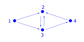
Figure 1. A Labelled Digraph

For $1\leq i\leq 4$, let $L_{i}(x)=\sum_{n\geq 1}\ell(n)x^{n}$ be the generating function for the lengths of paths going from vertex i to vertex 4, that is, $\ell_{i}(n)$ counts the number of paths of length $n$ from vertex $i$ to vertex $4$. Then ${\bf y}={\bf L}(x)$ satisfies the following system ${\bf y}={\bf G}(x,{\bf y})$:

$$y_{1} = x\cdot\big{(}y_{2}+y_{3}\big{)}$$

$$y_{2} = x\cdot y_{3}$$

$$y_{3} = x\cdot\big{(}y_{2}+1+y_{4}\big{)}$$

$$y_{4} = x\cdot y_{2}.$$

One has ${\bf G}(x,{\bf y})\unrhd 0$ and ${\bf G}(0,{\mathbf{0}})=J_{\bf G}(0,{\mathbf{0}})={\mathbf{0}}$, so the system is elementary. The associated elementary spectral system ${\bf Y}={\mathbf{\Gamma}}({\bf Y})$ is:

$$Y_{1} = 1+(Y_{2}\cup Y_{3})$$

$$Y_{2} = 1+Y_{3}$$

$$Y_{3} = 1\cup(1+(Y_{2}\cup Y_{4}))$$

$$Y_{4} = 1+Y_{2}.$$

To calculate the ${\mathfrak{m}}_{i}$ and ${\mathfrak{q}}_{i}$ for this system, first

$${\mathbf{\Gamma}}({\boldsymbol{\O}})\ =\ \left[\begin{array}[]{c}\O\\ \O\\ 1\\ \O\end{array}\right]\quad{\mathbf{\Gamma}}^{(2)}({\boldsymbol{\O}})\ =\ \left[\begin{array}[]{c}2\\ 2\\ 1\\ \O\end{array}\right]\quad{\mathbf{\Gamma}}^{(3)}({\boldsymbol{\O}})\ =\ \left[\begin{array}[]{c}\{2,3\}\\ 2\\ \{1,3\}\\ 3\end{array}\right]\quad{\mathbf{\Gamma}}^{(4)}({\boldsymbol{\O}})\ =\ \left[\begin{array}[]{c}\{2,3,4\}\\ \{2,4\}\\ \{1,3,4\}\\ 3\end{array}\right],$$

thus, by (23), ${\mathfrak{m}}=(2,2,1,3)$. For such a simple example one also easily finds the ${\mathfrak{m}}_{i}$ by inspection — ${\mathfrak{m}}_{i}$ is the length of the shortest path in Fig. 1 from vertex $i$ to vertex $4$.

To calculate the ${\mathfrak{q}}_{i}$ let

$$S_{j}\ :=\ \bigcup_{\bf u}G_{j,{\bf u}}+{\boldsymbol{\mathfrak{m}}}\star{\bf u}-{\mathfrak{m}}_{j},\quad\text{for }1\leq j\leq 4.$$

Then $S_{1}=\{0,1\}$, $S_{2}=\{0\}$, $S_{3}=\{0,2,3\}$, and $S_{4}=\{0\}$. The digraph in Fig. 1 is, conveniently, also the dependency digraph of the system, and $\{2,3,4\}$ is a strong component. From (24), ${\mathfrak{q}}_{i}=\gcd\bigcup_{i\rightarrow^{\star}j}S_{j}$, so ${\mathfrak{q}}_{1}=\gcd\big{(}S_{1}\cup S_{2}\cup S_{3}\cup S_{4}\big{)}=\gcd\{0,1,2,3\}=1$, and ${\mathfrak{q}}_{2}={\mathfrak{q}}_{3}={\mathfrak{q}}_{4}=\gcd\big{(}S_{2}\cup S_{3}\cup S_{4}\big{)}=\gcd\{0,2,3\}=1$.

4.4. Relaxing the Conditions on ${\bf G}(x,{\bf y})$

Recall that a power series system ${\bf y}={\bf G}(x,{\bf y})$ is elementary if (i) ${\bf G}(x,{\bf y})\unrhd{\mathbf{0}}$, (ii) ${\bf G}(0,{\mathbf{0}})={\mathbf{0}}$ and (iii) $J_{\bf G}(0,{\mathbf{0}})={\mathbf{0}}$.

The ‘elementary system’ requirement of Theorem 26 is usually true for power series systems ${\bf y}={\bf G}(x,{\bf y})$ arising in combinatorics — see, for example, the book [15] of Flajolet and Sedgewick, where most of the examples are such that $x$ is a factor of ${\bf G}(x,{\bf y})$, a property of ${\bf G}(x,{\bf y})$ which immediately guarantees that the second and third of the three conditions holds. The second condition, ${\bf G}(0,{\mathbf{0}})={\mathbf{0}}$, is essential if the solution ${\bf T}(x)$ provides generating functions $T_{i}(x)$ for combinatorial classes ${\mathcal{T}}_{i}$ since, in these cases, $T_{i}\subseteq{\mathbb{P}}$, so $0\notin T_{i}$, for an $i$.

Dropping the first requirement, that ${\bf G}(x,{\bf y})\unrhd{\mathbf{0}}$, leads to a difficult area of research where little is known, even with a single equation $y=G(x,y)$ — see the final sections of [1] for several remarks on the difficulties mixed signs in $G(x,y)$ pose when trying to determine the asymptotics of the coefficients $t(n)$ of a solution $y=T(x)$. Such mixed sign situations can arise naturally, for example when dealing with the construction ${\sf Set}$, which forms subsets of a given set of objects. The method developed in this paper for studying the spectra of the solutions $T_{i}(x)$ of a system ${\bf y}={\bf G}(x,{\bf y})$ very much depends on ${\bf G}(x,{\bf y})\unrhd{\mathbf{0}}$, in particular, claiming that ${\sf Spec}\big{(}{\bf G}_{\bf u}(x)\cdot{\bf T}(x)^{\bf u}\big{)}$ is equal to ${\bf G}_{\bf u}+{\bf u}\star{\bf T}$. This equality can fail with mixed signs, for example, the spectrum of $(1-x)\cdot(1+x+x^{2})$ is not the same as ${\sf Spec}(1-x)+{\sf Spec}(1+x+x^{2})$.

Thus the discussion regarding strengthening the results of the previous sections will be limited to dropping the third requirement, that $J_{\bf G}(0,{\mathbf{0}})={\mathbf{0}}$. This simply means that linear ${\bf y}$-terms with constant coefficients are permitted to appear in the $G_{i}(x,{\bf y})$, in which case a number of new possibilities can arise when classifying the solutions of such systems:

• There may be no (formal power series) solution, for example, $y=x+y$.

• There may be a solution, but not $\unrhd\,{\mathbf{0}}$, for example, $y=x+2y$.

• There may be infinitely many solutions, for example, $y_{1}=y_{2}$, $y_{2}=y_{1}$.

One can express the system ${\bf y}={\bf G}(x,{\bf y})$ as

$${\bf y}\ =\ {\bf G}(x,{\mathbf{0}})+J_{\bf G}(0,{\mathbf{0}})\cdot{\bf y}+{\bf H}(x,{\bf y}),$$

where

$${\bf H}(x,{\bf y})\ =\ \sum_{i=1}^{k}y_{i}\cdot{\bf H}_{i}(x,{\bf y})$$

with each ${\bf H}_{i}(x,{\bf y})\in{\mathbb{R}}[[x,{\bf y}]]_{0}^{k}$.

The obvious approach to such a system with $J_{\bf G}(0,{\mathbf{0}})\neq{\mathbf{0}}$ is to write it in the form

$$\big{(}I-J_{\bf G}(0,{\mathbf{0}})\big{)}\cdot{\bf y}\ =\ {\bf G}(x,0)+{\bf H}(x,{\bf y})$$

and solve for ${\bf y}$.

Definition 30 (of $\widehat{{\bf G}}$).

Given ${\bf G}(x,{\bf y})\unrhd{\mathbf{0}}$ with ${\bf G}(0,{\mathbf{0}})={\mathbf{0}}$, if the matrix $I-J_{\bf G}(0,{\mathbf{0}})$ has an inverse that is non-negative then let

$$\widehat{{\bf G}}(x,{\bf y})\ :=\ \Big{(}I-J_{\bf G}(0,{\mathbf{0}})\Big{)}^{-1}\cdot\Big{(}{\bf G}(x,{\mathbf{0}})+{\bf H}(x,{\bf y})\Big{)}.$$

Given a non-negative square matrix $M$, let $\Lambda(M)$ denote the largest real eigenvalue of $M$. (Note: From the Perron-Frobenius theory we know that a non-negative square matrix $M$ has a non-negative real eigenvalue, hence there is indeed a largest real eigenvalue $\Lambda(M)$, it is $\geq 0$, and $\Lambda(M)$ has a non-negative eigenvector.)

Theorem 31.

Let ${\bf G}(x,{\bf y})\in{\mathbb{R}}[[x,{\bf y}]]^{k}$ satisfy the two conditions

$${\bf G}(x,{\bf y})\unrhd{\mathbf{0}},\ \text{ and }{\bf G}(0,{\mathbf{0}})={\mathbf{0}}.$$

• Suppose $I-J_{\bf G}(0,{\mathbf{0}})$ has a non-negative inverse.

  (i) The system ${\bf y}=\widehat{{\bf G}}(x,{\bf y})$ is equivalent to the system ${\bf y}={\bf G}(x,{\bf y})$, that is, they have the same solutions $($but not necessarily the same dependency digraph$)$.

  (ii) $\widehat{{\bf G}}(x,{\bf y})$ is an elementary system.

  (iii) Consequently ${\bf T}(x):=\widehat{{\bf G}}^{(\infty)}(x,{\mathbf{0}})$ is the unique solution in ${\mathbb{R}}[[x]]_{0}$ of ${\bf y}={\bf G}(x,{\bf y})$ as well as of ${\bf y}=\widehat{{\bf G}}(x,{\bf y})$. The periodicity properties of ${\bf T}(x)$ are as stated in Theorem 26.

• Suppose that ${\bf G}^{(k)}(x,{\mathbf{0}})>{\mathbf{0}}$, that is, the associated system ${\bf Y}={\boldsymbol{\Gamma}}({\bf Y})$ of set equations is reduced. Then the following are equivalent:

  (i) $I-J_{\bf G}(0,{\mathbf{0}})$ has a non-negative inverse.

  (ii) ${\bf y}={\bf G}(x,{\bf y})$ has a solution ${\bf T}(x)\in{\sf Dom}_{0}[x]$.

  (iii) $\Lambda\big{(}J_{\bf G}(0,{\mathbf{0}})\big{)}<1$.

Proof.

(a): Given that $I-J_{\bf G}(0,{\mathbf{0}})$ has a non-negative inverse, one can transform either of ${\bf y}={\bf G}(x,{\bf y})$ and ${\bf y}=\widehat{{\bf G}}(x,{\bf y})$ into the other by simple operations that preserve solutions. It is routine to check that $\widehat{{\bf G}}(x,{\bf y})$ is an elementary system.

(b): Assume ${\bf G}^{(k)}(x,{\mathbf{0}})>{\mathbf{0}}$. (i) $\Rightarrow$ (ii) follows from (a). If (ii) holds then

$${\bf T}(x)\ =\ {\bf G}^{(k)}\big{(}x,{\bf T}(x)\big{)}\ \unrhd\ {\bf G}^{(k)}(x,{\mathbf{0}})\ >\ {\mathbf{0}}.$$

Let ${\bf v}\geq 0$ be a left eigenvector of $\Lambda\big{(}J_{{\bf G}^{(k)}}(0,{\mathbf{0}})\big{)}$. From

$${{\bf T}(x)}\ =\ {\bf G}^{(k)}(x,{\mathbf{0}})\,+\,J_{{\bf G}^{(k)}}(0,{\mathbf{0}})\cdot{{\bf T}(x)}\,+\,\widetilde{{\bf H}}\big{(}x,{{\bf T}(x)}\big{)},$$

one has

(25) $${\bf v}\cdot{\bf T}(x)\ =\ {\bf v}\cdot{\bf G}^{(k)}(x,{\mathbf{0}})\,+\,\Lambda\big{(}J_{{\bf G}^{(k)}}(0,{\mathbf{0}})\big{)}\cdot{\bf v}\cdot{\bf T}(x)\,+\,{\bf v}\cdot\widetilde{{\bf H}}\big{(}x,{{\bf T}(x)}\big{)}.$$

Since ${\bf T}(x)>{\mathbf{0}}$, one has ${\bf v}\cdot{\bf T}(x)$ and ${\bf v}\cdot{\bf G}^{(k)}(x,{\mathbf{0}})+\widetilde{{\bf H}}\big{(}x,{\bf T}(x)\big{)}$ are non-zero power series with non-negative coefficients, consequently (25) implies $\Lambda\big{(}J_{{\bf G}^{(k)}}(0,{\mathbf{0}})\big{)}<1.$ From $J_{{\bf G}^{(k)}}(0,{\mathbf{0}})=J_{{\bf G}}(0,{\mathbf{0}})^{k}$ it follows that $\Big{(}\Lambda\big{(}J_{{\bf G}}(0,{\mathbf{0}})\big{)}\Big{)}^{k}$ is an eigenvalue of $J_{{\bf G}^{(k)}}(0,{\mathbf{0}})$, and thus also $<1$. But this clearly implies $\Lambda\big{(}J_{{\bf G}}(0,{\mathbf{0}})\big{)}<1$, so (ii) $\Rightarrow$ (iii).

If (iii) holds, then by Neumann’s expansion theorem (see [17], p. 201), one knows that $I-J_{\bf G}(0,{\mathbf{0}})$ has an inverse, and $(I-J_{\bf G}(0,{\mathbf{0}})^{-1}=\sum_{n\geq 0}J_{\bf G}(0,{\mathbf{0}})^{n}$, a non-negative matrix. Thus (iii) $\Rightarrow$ (i). ∎

The condition ${\bf G}^{(k)}(x,{\mathbf{0}})>{\mathbf{0}}$ is the norm for power series systems in combinatorics since the $T_{i}(x)$ in the solution of ${\bf y}={\bf G}(x,{\bf y})$ are generating functions for non-empty classes ${\mathcal{T}}_{i}$.

It turns out (but will not be proved here) that for the calculation of the ${\mathfrak{m}}_{i}$ and ${\mathfrak{q}}_{i}$ one can use the formulas (23) and (24) of Theorem 26 with the original system ${\bf y}={\bf G}(x,{\bf y})$ as well as with the derived system ${\bf y}=\widehat{{\bf G}}(x,{\bf y})$. It can be useful to note that if the two hypotheses of Theorem 31 hold, then the condition ${\bf G}^{(k)}(x,{\mathbf{0}})>{\mathbf{0}}$ is equivalent to requiring that ${\bf G}^{(j)}(x,{\mathbf{0}})>{\mathbf{0}}$ hold for some $j$, $1\leq j\leq k$.

Remark 32.

The uniqueness of solutions ${\bf T}(x)$ in ${\mathbb{R}}[[x]]_{0}^{k}$ for power series systems ${\bf y}={\bf G}(x,{\bf y})$ satisfying the two hypotheses of Theorem 31 does not in general carry over to the associated spectral systems ${\bf Y}={\mathbf{\Gamma}}({\bf Y})$ when $J_{\bf G}(0,{\mathbf{0}})\neq{\mathbf{0}}$. For example, consider the consistent single equation system $y=G(x,y)$ where $G(x,y)=x^{2}+(1/2)y+xy$. The spectral system $Y={\Gamma}(Y)$ is $Y=2\cup Y\cup(1+Y)$, which has three solutions ${\mathbb{N}}$, $1+{\mathbb{N}}$, and $2+{\mathbb{N}}$. The elementary system $y=\widehat{G}(x,y)$ is $y=2x^{2}+2xy$; its spectral system is $Y=2\cup(1+Y)$, which has the unique solution $2+{\mathbb{N}}$.

4.5. A Non-linear Polynomial System

The following simple example uses all the tools developed so far.

Example 33.

Consider the class ${\mathcal{T}}$ of planar trees with blue and red colored nodes, defined by the conditions:

• every blue node that is not a leaf has exactly three subnodes, but not all of the same color;

• and every red node that is not a leaf has exactly two subnodes.

Let ${\mathcal{B}}$ be the collection of trees in ${\mathcal{T}}$ with the root colored blue, and likewise define ${\mathcal{R}}$ for the red-colored roots. Then, letting $\bullet_{B}$ be a blue-colored node and $\bullet_{R}$ a red-colored node, one has the equational specification

$${\mathcal{B}} = \{\bullet_{B}\}\ \cup\ \frac{\bullet_{B}}{{\mathcal{B}}+{\mathcal{R}}+{\mathcal{R}}}\ \cup\ \frac{\bullet_{B}}{{\mathcal{R}}+{\mathcal{B}}+{\mathcal{R}}}\ \cup\ \frac{\bullet_{B}}{{\mathcal{R}}+{\mathcal{R}}+{\mathcal{B}}}\ \cup\$$

$$\qquad\frac{\bullet_{B}}{{\mathcal{B}}+{\mathcal{B}}+{\mathcal{R}}}\ \cup\ \frac{\bullet_{B}}{{\mathcal{B}}+{\mathcal{R}}+{\mathcal{B}}}\ \cup\ \frac{\bullet_{B}}{{\mathcal{R}}+{\mathcal{B}}+{\mathcal{B}}}$$

$${\mathcal{R}} = \{\bullet_{R}\}\ \cup\ \frac{\bullet_{R}}{{\mathcal{T}}+{\mathcal{T}}}$$

$${\mathcal{T}} = {\mathcal{B}}+{\mathcal{R}}.$$

The three generating functions, $B(x)$ for ${\mathcal{B}}$, $R(x)$ for ${\mathcal{R}}$, and $T(x)$ for ${\mathcal{T}}$, are related by the system of equations:

$$B(x) = x\ +\ 3x\cdot B(x)\cdot R(x)^{2}\ +\ 3x\cdot B(x)^{2}\cdot R(x)$$

$$R(x) = x\ +\ x\cdot T(x)^{2}$$

$$T(x) = B(x)\ +\ R(x).$$

Thus $(B(x),R(x),T(x))$ gives a solution for $(y_{1},y_{2},y_{3})$ in the system of polynomial equations:

$$y_{1} = x\ +\ 3x\cdot y_{1}\cdot y_{2}^{2}\ +\ 3x\cdot y_{1}^{2}\cdot y_{2}$$

$$y_{2} = x\ +\ x\cdot y_{3}^{2}$$

$$y_{3} = y_{1}\ +\ y_{2}.$$

The spectra $B,R,T$ are related by the set-equations

$$B = 1\ \cup\ (1+B+2\star R)\ \cup\ (1+2\star B+R)$$

$$R = 1\ \cup\ (1+2\star T)$$

$$T = B\ \cup\ R,$$

so $(B,R,T)$ is a solution to the system of set-equations

$$Y_{1} = 1\ \cup\ 1+(Y_{1}+2\star Y_{2})\ \cup\ (1+2\star Y_{1}+Y_{2})$$

$$Y_{2} = 1\ \cup\ (1+2\star Y_{3})$$

$$Y_{3} = Y_{1}\ \cup\ Y_{2}.$$

Next,

$${\bf G}(x,y_{1},y_{2},y_{3})\ =\ \left[\begin{array}[]{c }x\,+\,3x\cdot y_{1}\cdot y_{2}^{2}\,+\,3x\cdot y_{1}^{2}\cdot y_{2}\\ x\,+\,x\cdot y_{3}^{2}\\ y_{1}\,+\,y_{2}\end{array}\right],$$

so

$${\bf G}^{(2)}(x,0,0,0)\ =\ \left[\begin{array}[]{c }6x^{4}\,+\,x\\ x\\ 2x\end{array}\right]\ >\ {\mathbf{0}}.$$

This implies ${\bf G}^{(k)}(x,{\mathbf{0}})>{\mathbf{0}}$, where $k=3$.

The Jacobian matrix $J_{\bf G}(x,{\bf y})$ is

$$J_{\bf G}(x,y_{1},y_{2},y_{3})\ =\ \left[\begin{array}[]{c c c}3xy_{2}^{2}\,+\,6xy_{1}y_{2}&6xy_{1}y_{2}\,+\,3xy_{1}^{2}&0\\ 0&0&2xy_{3}\\ 1&1&0\end{array}\right]$$

so

$$J_{\bf G}(x,0,0,0)\ =\ \left[\begin{array}[]{c c c}0&0&0\\ 0&0&0\\ 1&1&0\end{array}\right].$$

The eigenvalues of $J_{\bf G}(0,0,0,0)$ are the roots of $\det\big{(}\lambda I-J_{\bf G}(0,0,0,0)\big{)}=0$, that is, $\lambda^{3}=0$. Thus $\Lambda\big{(}J_{\bf G}(0,0,0,0)\big{)}=0<1$, so the system ${\bf y}={\bf G}(x,{\bf y})$ has a solution ${\bf T}(x)\in{\mathbb{R}}[[x]]_{0}^{3}$, and the solution is $>{\mathbf{0}}$ . The inverse of $I-J_{\bf G}(0,0,0,0)$ is a non-negative matrix:

$$\big{(}I-J_{\bf G}(0,0,0,0)\big{)}^{-1}\ =\ \left[\begin{array}[]{c c c}1&0&0\\ 0&1&0\\ 1&1&1\end{array}\right].$$

Thus

$$\widehat{{\bf G}}(x,{\bf y})\ =\ \left[\begin{array}[]{c }x\,+\,3xy_{1}y_{2}^{2}\,+\,3xy_{1}^{2}y_{2}\\ x\,+\,xy_{3}^{2}\\ 2x\,+\,3xy_{1}y_{2}^{2}\,+\,3xy_{1}^{2}y_{2}\,+\,xy_{3}^{2}\,+\,y_{1}\,+\,y_{2}\end{array}\right].$$

The spectral system ${\bf Y}=\widehat{{\mathbf{\Gamma}}}({\bf Y})$ is

$$Y_{1} = 1\cup\big{(}1\,+\,Y_{1}\,+\,2\star Y_{2}\big{)}\cup\big{(}1\,+\,2\star Y_{1}\,+\,Y_{2}\big{)}$$

$$Y_{2} = 1\,\cup\,\big{(}1\,+\,2\star Y_{3}\big{)}$$

$$Y_{3} = 1\,\cup\,\big{(}1\,+\,Y_{1}\,+\,2\star Y_{2}\big{)}\,\cup\,\big{(}1\,+\,2\star Y_{1}\,+\,Y_{2}\big{)}\,\cup\,\big{(}1\,+\,2\star Y_{3}\big{)}\cup Y_{1}\cup Y_{2}$$

5. General Systems

Recall that

$${\sf Dom}_{0}[x] = \big{\{}A(x)\in{\mathbb{R}}[x]:A(0)=0,A(x)\unrhd 0\big{\}}$$

$${\sf Dom}_{0}[x,{\bf y}] = \big{\{}{\bf G}(x,{\bf y})\in{\mathbb{R}}[x]^{k}:{\bf G}(x,{\bf y})\unrhd{\mathbf{0}},{\bf G}(0,{\mathbf{0}})={\mathbf{0}},J_{\bf G}(0,{\mathbf{0}})={\mathbf{0}}\big{\}}.$$

The systems ${\bf y}={\bf G}(x,{\bf y})$ considered so far are power-series systems. However these are not adequate to capture the scope of the popular constructions such as ${\sf MSet}$ (multiset) and ${\sf Cycle}$ used in combinatorial specifications—in particular one needs ${\sf MSet}$ in the study of monadic second–order classes in $\S$6.

If ${\mathcal{A}}$ and ${\mathcal{B}}$ are two combinatorial classes with the same generating function, that is, $A(x)=B(x)$, then ${\sf MSet}({\mathcal{A}})$ and ${\sf MSet}({\mathcal{B}})$ have the same generating function; likewise for the construction ${\sf Cycle}$. Such constructions are called admissible in Flajolet and Sedgewick [15]. In the case of ${\sf MSet}$, the generating function for ${\sf MSet}({\mathcal{A}})$ is

$$\exp\Big{(}\sum_{m\geq 1}A(x^{m})/m\Big{)}-1.$$

Ordinary generating functions $A(x)$ have integer coefficients; the operator ${\sf MSet}$ is extended to all $A(x)\in{\sf Dom}_{0}[x]$ by the same expression:

$${\sf MSet}(A(x))\ :=\ \exp\Big{(}\sum_{m\geq 1}A(x^{m})/m\Big{)}-1.$$

This operator cannot be expressed by a power series in $A(x)$, so specifications using ${\sf MSet}$ do not, in general, lead to elementary systems.

The operations and constructions/operators considered here are (see [15] or [1]):

• the constant $\bullet$ (a single node) corresponds to the polynomial $x$ in generating functions

• the construction $union$ (disjoint union) corresponds to the operation of $+$ (addition) for generating functions

• the construction $+$ (disjoint sum) corresponds to the operation $\times$ (product) for generating functions

• the construction/operator ${\sf Seq}$ (sequence)

• the construction/operator ${\sf MSet}$ (multiset)

• the construction/operator ${\sf Cycle}$ (cycle)

• the construction/operator ${\sf DCycle}$ (directed cycle)

Items (d)–(g) are called the standard constructions. A standard construction $\Theta$ can be restricted to a set of positive integers $J$, giving the construction $\Theta_{J}$, the meaning of which is that $\Theta_{J}({\mathcal{A}})$ consists of all objects that one can construct by applying $\Theta$ to only $J$-many objects from ${\mathcal{A}}$ (repeats allowed). Thus ${\sf MSet}_{\sf Even}({\mathcal{A}})$ gives all multisets consisting of an even number of objects from ${\mathcal{A}}$. The operators $J\star$, for $J\subseteq{\mathbb{N}}$, are precisely the operators ${\sf MSet}_{J}$, so the star operation ($\star$) is included in the above list.

Definition 34.

Let ${\mathcal{C}}$ be the collection of combinatorial classes. A construction

$${\Theta}:{\mathcal{C}}^{k}\rightarrow{\mathcal{C}}^{m}$$

is admissible iff:

whenever two $k$-tuples of combinatorial classes ${\boldsymbol{\mathcal{A}}}$ and ${\boldsymbol{\mathcal{B}}}$ have the same $k$-tuples of generating functions ${\bf A}(x)$ and ${\bf B}(x)$ then the $m$-tuple of combinatorial classes ${{\mathbf{\Theta}}}({\boldsymbol{\mathcal{A}}})$ and ${{\mathbf{\Theta}}}({\boldsymbol{\mathcal{B}}})$ also have the same $n$-tuples of generating functions.

The operator from ${\sf Dom}_{0}[x]^{k}$ to ${\sf Dom}_{0}[x]^{m}$ induced by such a construction is also designated by ${\mathbf{\Theta}}$.

A variant of this definition is needed for the study of spectra of solutions to systems of equations.

Definition 35.

An operator

$${\mathbf{\Theta}}:{\sf Dom}_{0}[x]^{k}\rightarrow{\sf Dom}_{0}[x]^{m},$$

is spectrally admissible provided:

whenever two $k$-tuples ${\bf A}(x)$ and ${\bf B}(x)$ from ${\sf Dom}_{0}[x]^{k}$ have the same spectra, that is, ${\bf A}={\bf B}$, then ${\mathbf{\Theta}}({\bf A}(x))$ and ${\mathbf{\Theta}}\big{(}{\bf B}(x)\big{)}$ also have the same spectra, that is, ${\sf Spec}\Big{(}{\mathbf{\Theta}}\big{(}{\bf A}(x)\big{)}\Big{)}={\sf Spec}\Big{(}{\mathbf{\Theta}}\big{(}{\bf B}(x)\big{)}\Big{)}.$

The operator from ${\rm Su}({\mathbb{N}})^{k}$ to ${\rm Su}({\mathbb{N}})^{m}$, where ${\rm Su}({\mathbb{N}})$ is the set of subsets of ${\mathbb{N}}$, induced by a spectrally admissible operator ${\mathbf{\Theta}}$ is designated by ${\mathbf{\Gamma}}_{\mathbf{\Theta}}$.

Lemma 36.

Each ${\bf G}(x,{\bf y})\in{\sf Dom}_{J0}[x,{\bf y}]^{k}$ defines an operator on ${\sf Dom}_{0}[x]^{k}$ that is both admissible and spectrally admissible. Such operators are called elementary operators. As a spectrally admissible operator, ${\bf G}(x,{\bf y})$ induces a set-operator $($on ${\rm Su}({\mathbb{N}})^{k}$, the set of $k$-tuples of subsets of ${\mathbb{N}}$$)$, namely

$${\mathbf{\Gamma}}:{\bf A}\mapsto\bigcup_{{\bf u}\in{\mathbb{N}}^{k}}{\bf G}_{i,{\bf u}}+({\bf u}\star{\bf A}).$$

Definition 37.

Two spectrally admissible operators ${\mathbf{\Theta}}$ and ${\mathbf{\Theta}}^{\prime}$ on ${\sf Dom}_{0}[x]^{k}$ are spectrally equivalent if they give the same set-operator, that is, for all ${\bf A}(x)\in{\sf Dom}_{0}[x]^{k}$,

$${\sf Spec}\big{(}{\mathbf{\Theta}}\big{(}{\bf A}(x)\big{)}\big{)}\ =\ {\sf Spec}\big{(}{\mathbf{\Theta}}^{\prime}\big{(}{\bf A}(x)\big{)}\big{)}.$$

The standard admissible operators (and their restrictions) map ${\sf Dom}_{0}[x]$ to itself, hence $k=m=1$ in such cases. However the elementary operators require that one take arbitrary $k\geq 1$ into consideration.

In addition to the (restrictions of the) standard constructions $\Theta$ being admissible, they are spectrally admissible. A simplifying feature of working with spectrally admissible operators is that they can often be better understood by replacing them with equivalent elementary operators.

Theorem 38 (Systems based on Spectrally Admissible Operators).

• Elementary operators ${\bf G}(x,{\bf y})$ and restrictions $\Theta_{J}$ of the standard operators $\Theta$ are spectrally admissible.

• The restriction $\Theta_{J}(y)$ of a standard operator $\Theta$ is spectrally equivalent to the elementary operator $\displaystyle\sum_{j\in J}y^{j}$, and ${\sf Spec}\big{(}\Theta_{J}\big{(}A(x)\big{)}\big{)}=J\star A$.

• The sum $\Theta_{1}+\Theta_{2}$, product $\Theta_{1}\cdot\Theta_{2}$ and composition $\Theta_{1}\circ\Theta_{2}$ of spectrally admissible operators is spectrally admissible.

• Any combination of elementary operators and restrictions of standard operators — using the operations of sum, product and composition — yields an operator that is spectrally admissible and spectrally equivalent to an elementary operator.

• If ${\mathbf{\Theta}}({\bf y})$ is spectrally equivalent to ${\mathbf{\Theta}}^{\prime}({\bf y})$ then

  $${\sf Spec}\big{(}{\mathbf{\Theta}}^{(\infty)}({\boldsymbol{\O}})\big{)}\ =\ {\sf Spec}\big{(}{\mathbf{\Theta}}^{\prime(\infty)}({\boldsymbol{\O}})\big{)}.$$

• Let ${\bf y}={\mathbf{\Theta}}({\bf y})$ be a system with solution ${\bf T}(x)\in{\sf Dom}_{0}[x]^{k}$, where the operators $\Theta_{i}$ are combinations as described in item (d). By (d), ${\mathbf{\Theta}}$ is spectrally equivalent to an elementary operator ${\bf G}(x,{\bf y})$. Let ${\bf U}(x)$ be the unique solution to ${\bf y}={\bf G}(x,{\bf y})$ guaranteed by Theorem 26. Then ${\bf T}={\bf U}$.

  Thus periodicity properties for the $T_{i}(x)$ can be deduced by applying Theorem 26 to ${\bf y}={\bf G}(x,{\bf y})$.

Proof.

Items (a) through (e) are straightforward. For item (f), the operators $\Theta_{i}({\bf Y})$ are spectrally equivalent to an elementary operator by (d). From the spectral equivalence of the operators ${\mathbf{\Theta}}({\bf y})$ and ${\bf G}(x,{\bf y})$ and the fact that ${\bf T}(x)$ is a solution of ${\bf y}={\mathbf{\Theta}}({\bf y})$, one has

$${\bf T}\ =\ {\sf Spec}\big{(}{\mathbf{\Theta}}\big{(}{\bf T}(x)\big{)}\big{)}\ =\ {\sf Spec}\big{(}{\bf G}\big{(}x,{\bf T}(x)\big{)}\big{)}\ =\ {\mathbf{\Gamma}}({\bf T}),$$

where ${\boldsymbol{\Gamma}}$ is the set operator corresponding to ${\bf G}(x,{\bf y})$. So ${\bf T}$ is a solution of ${\bf Y}={{\mathbf{\Gamma}}}\big{(}{\bf Y}\big{)}.$ Now ${\bf U}(x)={\bf G}({\bf U}(x))$ implies that ${\bf U}$ is also a solution of ${\bf Y}={{\mathbf{\Gamma}}}\big{(}{\bf Y}\big{)}.$ Theorem 21 says that the elementary system ${\bf Y}={\mathbf{\Gamma}}({\bf Y})$ has a unique solution, so ${\bf U}={\bf T}$. Consequently the periodicity properties of ${\bf T}$ are those of ${\bf U}$, and thus Theorem 26 can be used to analyze ${\bf T}$. ∎

The next example illustrates the methods for determining the periodicity parameters for the power series solution ${\bf T}(x)$ of a general equational system ${\bf y}={\mathbf{\Theta}}({\bf y})$ using a specification of ‘structured’ trees, where (some or all of) the nodes immediately below a node can be given a structure, such as a cycle or a sequence.

Example 39.

Let ${\mathcal{T}}$ be the class of two-colored $($red,blue$)$ ‘structured’ trees which satisfies the following conditions:

• A red node must have a cycle consisting of a positive even number of red nodes, or 6 blue nodes, at least 3 of the blue nodes being leaves, immediately below it;

• A blue node that is not a leaf has a multiset consisting of a prime number of red nodes immediately below it, plus a sequence of blue nodes whose number is congruent to 4 mod 6.

Letting ${\mathcal{R}}$ be the members of ${\mathcal{T}}$ with a red root, and ${\mathcal{B}}$ those with a blue root, one has the specification

$${\mathcal{R}} = \frac{\bullet_{R}}{{\sf Cycle}_{\sf PosEven}({\mathcal{R}})}\ \cup\ \frac{\bullet_{R}}{3\bullet_{B}\ +\ {\sf MSet}_{3}({\mathcal{B}})}$$

$${\mathcal{B}} = \{\bullet_{B}\}\ \cup\ \frac{\bullet_{B}}{{\sf MSet}_{{\sf Primes}}({\mathcal{R}})\ +\ {\sf Seq}_{4+6\cdot{\mathbb{N}}}({\mathcal{B}})}$$

$${\mathcal{T}} = {\mathcal{R}}\cup{\mathcal{B}}.$$

The associated spectral system is

$$Y_{1} = (1+{\sf PosEven}\star Y_{1})\ \cup\ (4+3\star Y_{2})$$

$$Y_{2} = 1\cup\Big{(}1+{\sf Primes}\star Y_{1}+(4+6\cdot{\mathbb{N}})\star Y_{2}\Big{)}$$

$$Y_{3} = Y_{1}\cup Y_{2}$$

with solution $(Y_{1},Y_{2},Y_{3})=(R,B,T)$. This is not an elementary system $($because of the linear terms in the right side of the third equation$)$, but nonetheless the solution is unique. Note that $\{1,2\}$ is a strong component of the dependency digraph.

To determine the periodicity parameters for ${\mathcal{T}}$ it suffices to determine them for ${\mathcal{B}}$ and ${\mathcal{R}}$ and apply Proposition 8, since ${\mathfrak{m}}(T)={\mathfrak{m}}(R\cup B)$ and ${\mathfrak{q}}(T)={\mathfrak{q}}(R\cup B)$. The first two equations form an elementary system, and one has:

$${\mathbf{\Gamma}}(Y_{1},Y_{2}) = \left(\begin{array}[]{c c}(1+{\sf PosEven}\star Y_{1})\ \cup\ (4+3\star Y_{2})\\ 1\cup\Big{(}1+{\sf Primes}\star Y_{1}+(4+6\cdot{\mathbb{N}})\star Y_{2}\Big{)}\end{array}\right)$$

$${\mathbf{\Gamma}}(\O,\O) = \left(\begin{array}[]{c c}\O\\ 1\end{array}\right)$$

$${\mathbf{\Gamma}}^{(2)}(\O,\O) = \left(\begin{array}[]{c c}7\\ 1\end{array}\right).$$

Thus ${\boldsymbol{\mathfrak{m}}}:=({\mathfrak{m}}_{1},{\mathfrak{m}}_{2})=(7,1)$.

Writing

$$\Gamma_{i}(Y_{1},Y_{2})=\bigcup_{{\bf u}\in{\mathbb{N}}^{2}}G_{i,{\bf u}}+(u_{1}\star Y_{1}+u_{2}\star Y_{2})$$

one has

$$G_{1,{\bf u}} = \begin{cases}1&\text{if }u_{1}\in{\sf PosEven}\text{ and }u_{2}=0\\ 4&\text{if }u_{1}=0\text{ and }u_{2}=3\\ \O&\text{otherwise}\end{cases}$$

$$G_{2,{\bf u}} = \begin{cases}1&\text{if }(u_{1}=u_{2}=0)\text{ or }(u_{1}\in{\sf Primes}\text{ and }u_{2}\equiv 4\text{ mod }6)\\ \O&\text{otherwise}.\end{cases}$$

Now ${\bf u}\star{\boldsymbol{\mathfrak{m}}}=7u_{1}+u_{2}$, so

$$G_{1,{\bf u}}+{\bf u}\star{\boldsymbol{\mathfrak{m}}}-{\mathfrak{m}}_{1} = \begin{cases}7u_{1}+u_{2}-6&\text{if }(u_{1}\in{\sf PosEven}\text{ and }u_{2}=0)\\ 7u_{1}+u_{2}-3&\text{if }u_{1}=0\text{ and }u_{2}=3\\ \O&\text{otherwise}\end{cases}$$

$$G_{2,{\bf u}}+{\bf u}\star{\boldsymbol{\mathfrak{m}}}-{\mathfrak{m}}_{2} = \begin{cases}7u_{1}+u_{2}&\text{if }(u_{1}=u_{2}=0)\text{ or }(u_{1}\in{\sf Primes}\text{ and }u_{2}\equiv 4\text{ mod }6)\\ \O&\text{otherwise}.\end{cases}$$

From this one has

$$\gcd\bigcup_{\bf u}\big{(}G_{1,{\bf u}}+{\bf u}\star{\boldsymbol{\mathfrak{m}}}-{\mathfrak{m}}_{1}\big{)} = \gcd\{7u_{1}-6:u_{1}\in{\sf PosEven}\}\ =\ 2$$

$$\gcd\bigcup_{\bf u}\big{(}G_{2,{\bf u}}+{\bf u}\star{\boldsymbol{\mathfrak{m}}}-{\mathfrak{m}}_{2}\big{)} = \gcd\{7u_{1}+u_{2}:u_{1}\in{\sf Primes}\text{ and }u_{2}\equiv 4\text{ mod }6\}\ =\ 1$$

Since the two equation system is irreducible, that is, $i\rightarrow^{+}j$ for all vertices $i,j$, one has

$${\mathfrak{q}}_{1} = {\mathfrak{q}}_{2}\ =\ \gcd\bigcup_{\bf u}\bigcup_{i=1}^{2}G_{i,{\bf u}}+{\bf u}\star{\boldsymbol{\mathfrak{m}}}-{\mathfrak{m}}_{i}$$

$$= \gcd(2,1)\ =\ 1.$$

Using Proposition 8, the above calculations give

$${\mathfrak{m}}_{3} = \min({\mathfrak{m}}_{1},{\mathfrak{m}}_{2})\ =\ \min(7,1)\ =\ 1$$

$${\mathfrak{q}}_{3} = \gcd({\mathfrak{q}}_{1},{\mathfrak{q}}_{2},{\mathfrak{m}}_{1}-{\mathfrak{m}}_{2})\ =\ \gcd(1,1,6)\ =\ 1.$$

In summary, $({\mathfrak{m}}(R),{\mathfrak{m}}(B),{\mathfrak{m}}(T))=(7,1,1)$ and $({\mathfrak{q}}(R),{\mathfrak{q}}(B),{\mathfrak{q}}(T))=(1,1,1)$.

6. Monadic Second Order Classes

At present there are two major approaches to describing broad collections of combinatorial structures: (1) combinatorialists (see, for example, [15]) prefer to look at specifications that are based on constructions like sequences, cycles and multisets, whereas (2) logicians prefer to look at classes that are defined by sentences in a formal logic.

When working with relational structures like graphs and trees, logicians have found it worthwhile to strengthen first-order logic to monadic second-order logic (MSO logic). The primary reason for the interest in MSO logic is the powerful connection between Ehrenfeucht-Fraïssé games and sentences of a given quanifier rank. These games, although very combinatorial in nature, are not widely used in the combinatorics community.

6.1. Regular Languages

A set ${\mathcal{L}}$ of words over an $m$-letter alphabet is a regular language if it is precisely the set of words accepted by some finite state deterministic automaton. A word is accepted by such an automaton if, starting at state 0, one can follow a path to a final state with the successive edges of the path spelling out the word. Let the states of the automaton be $S_{0},\ldots,S_{k}$, and for each state $S_{i}$ let ${\mathcal{L}}_{i}$ be the set of words traversed when going from vertex $i$ to a final state vertex. Then one sees that ${\mathcal{L}}_{i}$ is the union of the classes $a_{ij}{\mathcal{L}}_{j}$ where $i\rightarrow j$ is an edge in the automaton labeled by the letter $a_{ij}$ from the alphabet. This leads to equations of a particularly simple form for the generating functions and the spectra, namely for $1\leq i\leq k$,

$$L_{i}(x) = x\cdot\big{(}c_{i}+\sum_{i\rightarrow j}L_{j}(x)\big{)}$$

$$L_{i} = A_{i}\cup\big{(}1+\bigcup_{i\rightarrow j}L_{j}\big{)}.$$

One of the first big successes for MSO was Büchi’s Theorem connecting the regular languages studied by computer scientists with classes of colored digraphs defined by MSO sentences. To see how this connection is made, simply note that a word on $m$ letters corresponds to an $m$-colored linear digraph $(D,\rightarrow,C_{1},\ldots,C_{m})$, and thus a language on an $m$-letter alphabet can be thought of as a class of $m$-colored linear digraphs.

Theorem 40 (Büchi [5], 1960).

MSO classes of colored linear digraphs are precisely the regular languages.

The theory of the generating functions for MSO classes of colored linear digraphs was worked out, in the context of regular languages, by Berstel [4], 1971 (his results were soon augmented by Soittola [21], 1976). Given a regular language ${\mathcal{R}}$, one can partition it into classes ${\mathcal{R}}_{i}$ such that the generating functions $R_{i}(x)$ satisfy a system of linear equations ${\bf y}=x(C+M\cdot{\bf y})$, where $C$ is a 0,1-column matrix, and $M$ is a 0,1-square matrix. The equations are easily read off a finite state deterministic automata that accepts the language; one writes down a system of equations for the paths in the automata, similar to the situation in Example 29. The equations have a particularly simple linear form—the spectra $R_{i}$ are eventually periodic, and by Cramer’s rule, the generating functions $R_{i}(x)$ are rational functions; also they are given by ${\bf R}(x)=x\cdot\big{(}I-xM\big{)}^{-1}\cdot C.$ Berstel showed that each $R_{i}(x)$ decomposes into a finite number of $R_{ij}(x)$, each $R_{ij}$ being either finite or eventually an arithmetical progression. For those which are not finite there are polynomials $P_{ijk}(n)$ and complex numbers $\beta_{ijk}=\beta_{ij}\cdot\omega_{ij}^{k}$, with $\beta_{ij}$ a positive real and $\omega_{ij}$ a root of unity, such that, on the set $R_{ij}$, one has the coefficients $r_{ij}(n)$ having an exact polynomial-exponential form, and polynomial-exponential asymptotics, given by (see [15], p. 302):

$$r_{ij}(n) = \sum_{k}P_{ijk}(n)\beta_{ijk}^{n}\quad\text{on the set }R_{ij}$$

$$\sim P_{ij0}(n)\beta_{ij}^{n}\quad\text{on the set }R_{ij}.$$

This study of the generating functions for MSO classes of colored linear digraphs provides the Berstel Paradigm, a successful analysis that one would like to see paralleled in the study of all MSO classes of colored trees. For example, can one show that the generating functions $T(x)$ of such classes decompose into a polynomial and finitely many “nice” functions $T_{i}(x)$, with each spectrum $T_{i}$ being an arithmetical progression?

6.2. Trees and Forests

When speaking of structures, in particular the models of a sentence $\varphi$, it will be understood that only finite structures are being considered.

A tree ${\bf T}=(T,<)$ is a poset such that: (i) there is a unique maximal element ${\sf rt}({\bf T})$ called the root of the tree, and (ii) every interval $[a,{\sf rt}({\bf T})]$ is linear. A forest ${\bf F}=(F,<)$ is a poset whose components are trees.

A forest ${\bf F}$ is determined (up to isomorphism) by the number of each (isomorphism type of) tree appearing in it, thus by its counting function $\nu_{\bf F}:{\rm TREES}\rightarrow{\mathbb{N}}$.

One can combine two forests ${\bf F}_{1}$ and ${\bf F}_{2}$ into a single forest ${\bf F}_{1}+{\bf F}_{2}$ which is determined up to isomorphism by $\nu_{{\bf F}}=\nu_{{\bf F}_{1}}+\nu_{{\bf F}_{2}}$. Extend this operation to classes ${\mathcal{F}}$ of forests by ${\mathcal{F}}_{1}+{\mathcal{F}}_{2}=\{{\bf F}_{1}+{\bf F}_{2}:{\bf F}_{i}\in{\mathcal{F}}_{i}\}$. The ideal class ${\mathcal{O}}$ of forests is introduced with the properties ${\mathcal{O}}\cup{\mathcal{F}}={\mathcal{O}}+{\mathcal{F}}={\mathcal{F}}$ (it is introduced solely as a notational device to smooth out the presentation).

Define the operation $\star$ between non-empty subsets $A$ of ${\mathbb{N}}$ and non-empty classes ${\mathcal{F}}$ of forests by

$$n\star{\mathcal{F}} = \begin{cases}{\mathcal{O}}&\text{if }n=0\\ \underbrace{{\mathcal{F}}+\cdots+{\mathcal{F}}}_{n-\text{fold}}&\text{if }n\geq 1\end{cases}$$

$$A\star{\mathcal{F}} = \bigcup_{a\in A}a\star{\mathcal{F}}.$$

6.3. Compton’s Specification of MSO Classes of Trees

${\bf F}_{1}\equiv_{q}^{\rm MSO}{\bf F}_{2}$ means that ${\bf F}_{1}$ and ${\bf F}_{2}$ satisfy the same MSO sentences of quantifier rank $q$. $\equiv_{q}^{\rm MSO}$ is an equivalence relation on ${\mathcal{F}}$ of finite index. In the following, when given a MSO class ${\mathcal{F}}$ of forests, it will be assumed that $q$ has been chosen large enough so (i) ${\mathcal{F}}$ is definable by a MSO sentence of quantifier depth $q$, and (ii) that there are MSO sentences of quantifier depth $q$ to express “is a tree”, “is a forest”. Then ${\rm TREES}$ is a union of $\equiv_{q}^{\rm MSO}$ classes of forests, say ${\rm TREES}={\mathcal{T}}_{1}\cup\cdots\cup{\mathcal{T}}_{r}$. If ${\mathcal{T}}_{i}$ has a 1-element tree in it then no other tree is in ${\mathcal{T}}_{i}$. Assume that there are $m$ colors, and let $\bullet_{i}$ denote the 1-element tree of color $i$, and assume ${\mathcal{T}}_{i}=\{\bullet_{i}\}$ for $1\leq i\leq m$. These are the only ${\mathcal{T}}_{i}$ with a one-element member, and all trees in any given ${\mathcal{T}}_{i}$ have the same root-color, say $i^{\prime}$.

Given a tree ${\bf T}$ with more than one element, let $\partial{\bf T}$ be the forest that results from removing the root ${\sf rt}({\bf T})$ from ${\bf T}$; and given any forest ${\bf F}$, let $\bullet_{i}/{\bf F}$ be the tree that results by adding a root of color $i$ to the forest. The operation $\partial$ is extended in the obvious manner to $\partial{\mathcal{T}}$ for any non-empty class ${\mathcal{T}}$ of trees that does not have a one-element tree in it; and the operation of adding a root of color $i$ to a forest is extended to $\bullet_{i}/{\mathcal{F}}$ for any non-empty class ${\mathcal{F}}$ of forests.

Lemma 41.

Let $q$ be a positive integer.

• The operations of disjoint union and $\bullet_{i}\big{/}$ preserve $\equiv_{q}^{\sf MSO}$, that is,

  $\displaystyle T_{i}\equiv_{q}^{\sf MSO}T_{i}^{\prime}\ \Rightarrow\ \sum_{i}T_{i}\equiv_{q}^{\sf MSO}\sum_{i}T_{i}^{\prime}$, and

  $\displaystyle F\equiv_{q}^{\sf MSO}F^{\prime}\ \Rightarrow\ \bullet_{i}/F\equiv_{q}^{\sf MSO}\bullet_{i}/F^{\prime}$, for $1\leq i\leq m$.

• There is a constant $C_{q}$ such that for all trees $T$ and all $n\geq C_{q}$ one has $n\star T\equiv_{q}^{\sf MSO}C_{q}\star T$.

• There is a decision procedure to determine if $F_{1}\equiv_{q}^{\sf MSO}F_{2}$.

Proof.

One can find a discussion of the first item of (a), as well as item (b), in [6], based on E-F games. Use E-F games for (c) as well. (a)–(c) are basic tools of Gurevich and Shelah ([16], 2003). ∎

The next lemma gives the crucial structure result for MSO classes of forests.

Lemma 42.

Let ${\mathcal{F}}$ be a MSO class of forests defined by a sentence of quantifier rank $q$. Then there is a finite set ${\mathbb{S}}$ of $r$-tuples $S=(S_{i})$ of cofinite or non-empty finite subsets $S_{i}$ of ${\mathbb{N}}$ such that

$${\mathcal{F}}\ =\ \bigcup_{S\in{\mathbb{S}}}\sum_{\begin{subarray}{c}j=1\\ S_{j}\neq\{0\}\end{subarray}}^{r}S_{j}\star{\mathcal{T}}_{j}.$$

Proof.

Let $C_{q}$ be as in Lemma 41. A routine application of Ehrenfeucht-Fraïssé games shows that for any two $r$-tuples $(n_{i})$ and $(n_{i}^{\prime})$ of non-negative integers with $n_{i}\geq C_{q}$ iff $n_{i}^{\prime}\geq C_{q}$, one has every member of $\sum_{i}n_{i}\star{\mathcal{T}}_{i}$ equivalent modulo $\equiv_{q}^{\rm MSO}$ to every member of $\sum_{i}n_{i}^{\prime}\star{\mathcal{T}}_{i}$.

Thus ${\mathcal{F}}$ decomposes into a (disjoint) union of finitely many classes $\sum_{i=1}^{r}S_{i}\star{\mathcal{T}}_{i}$ where each $S_{i}$ is either a singleton $\{n_{i}\}$ with $1\leq n_{i}\leq m$ or the cofinite set $\{n:n\geq C_{q}\}$. ∎

Lemma 43.

For $m<i\leq r$, the class of forests $\partial{\mathcal{T}}_{i}$ is definable by a MSO sentence of quantifier rank $q$.

Proof.

$\partial{\mathcal{T}}_{i}$ is closed under $\equiv_{q}^{\rm MSO}$ since Lemma 41 shows ${\bf F}_{1}\equiv_{q}^{\rm MSO}{\bf F}_{2}$ implies $\bullet_{i}\big{/}{\bf F}_{1}\equiv_{q}^{\rm MSO}\bullet_{i}\big{/}{\bf F}_{2}$, thus ${\bf F}_{1}\equiv_{q}^{\rm MSO}{\bf F}_{2}$ and ${\bf F}_{1}\in\partial{\mathcal{T}}_{i}$ imply ${\bf F}_{2}\in\partial{\mathcal{T}}_{i}$. ∎

Theorem 44 (Compton, see [24]).

Let ${\mathcal{T}}$ be a class of $m$-colored trees defined by a MSO sentence of quantifier depth $q$. Then:

• ${\mathcal{T}}$ is a union of some of the ${\mathcal{T}}_{i}$, and

• the ${\mathcal{T}}_{i}$ satisfy a system of equations

  $$\Sigma_{q}:\ \left\{\begin{array}[]{r c l}{\mathcal{T}}_{1}&=&\Phi_{1}\big{(}{\mathcal{T}}_{1},\ldots,{\mathcal{T}}_{r}\big{)}\\ &\vdots&\\ {\mathcal{T}}_{r}&=&\Phi_{r}\big{(}{\mathcal{T}}_{1},\ldots,{\mathcal{T}}_{r}\big{)},\end{array}\right.$$

where $\Phi_{i}\big{(}{\mathcal{T}}_{1},\ldots,{\mathcal{T}}_{r}\big{)}$ is $\{\bullet_{i}\}$ for $1\leq i\leq m$, and for $i>m$ it has the form

(29) $$\bullet_{i^{\prime}}\bigg{/}\bigcup_{S\in{\mathbb{S}}_{i}}\sum_{j=1}^{r}S_{j}\star{\mathcal{T}}_{j}$$

with each ${\mathbb{S}}_{i}$ being a finite set of $r$-tuples $S=(S_{1},\ldots,S_{r})$, with each $S_{j}$ a cofinite or non-empty finite subset of $\mathbb{N}$.

Proof.

(a) is obviously true. For (b) note that for $m<i\leq r$, ${\mathcal{T}}_{i}=\bullet_{i}\big{/}\partial{\mathcal{T}}_{i}$. Lemma 43 says $\partial{\mathcal{T}}_{i}$ is definable by a MSO sentence of quantifier rank $q$. Then Lemma 42 shows that $\partial{\mathcal{T}}_{i}$ can be expressed in a particular form. One only needs to attach the root $\bullet_{i^{\prime}}$ to have (29). ∎

Applying ${\sf Spec}$ to $\Sigma_{q}$ gives a system of set-equations for the spectra of the classes ${\mathcal{T}}_{i}$:

Corollary 45.

For ${\mathcal{T}}$ as in Compton’s Theorem, ${\sf Spec}({\mathcal{T}})$ is a union of some of the ${\sf Spec}({\mathcal{T}}_{i})$, and

(30) $$\displaystyle{\sf Spec}({\mathcal{T}}_{i}) = \begin{cases}\{1\}&\text{for }1\leq i\leq m\\ \displaystyle\{1\}+\bigcup_{S\in{\mathbb{S}}_{i}}\sum_{j=1}^{r}S_{j}\star{\sf Spec}({\mathcal{T}}_{j})&\text{for }m<i\leq r.\end{cases}$$

Remark 46.

Compton [9] described his equational specification for the minimal MSO classes of trees of quantifier depth $q$ to Alan Woods during a visit to Yale in 1986; at the time Woods was a PostDoc at Yale. Evidently Compton regarded such an equational specification for trees as a straightforward generalization of the earlier work of Büchi, which showed that regular languages were precisely the MSO classes of $m$-colored linear trees.

6.4. The dependency digraph of $\Sigma_{q}$

The dependency digraph $D_{\mathfrak{q}}$ for $\Sigma_{q}$ is defined parallel to the definition for systems of set-equations. $D_{q}$ has vertices $1,\ldots,r$ and, referring to (30), directed edges given by $i\rightarrow j$ iff there is a $S\in{\mathbb{S}}_{i}$ such that $S_{j}\neq\{0\}$. One defines a height function on $D_{q}$ by setting $h(i)=0$ for $1\leq i\leq m$, and then for $m<i\leq r$ use the inductive definition $h(i)=1+\max\{h(j):i\rightarrow^{+}j,\text{ but not }j\rightarrow^{+}i\}$.

Corollary 47.

The spectrum of a MSO class ${\mathcal{T}}$ of $m$-colored trees is eventually periodic.

Proof.

It suffices to prove this result for the ${\mathcal{T}}_{i}$ in view of Lemma 6 (which guarantees that eventual periodicity is preserved by finite union). For $1\leq i\leq m$ this is trivial. So suppose $m<i\leq r$, and note that whenever $j\rightarrow k$ one has ${\sf Spec}({\mathcal{T}}_{j})\supseteq p_{jk}+{\sf Spec}({\mathcal{T}}_{k})$ for some positive integer $p_{jk}$, by (30). Thus $i\rightarrow^{+}j$ implies the same conclusion. If $[i]\neq\O$ then $i\rightarrow^{+}i$, so ${\sf Spec}({\mathcal{T}}_{i})\supseteq p+{\sf Spec}({\mathcal{T}}_{i})$ for some $p\in{\mathbb{P}}$, so ${\sf Spec}({\mathcal{T}}_{i})$ is actually periodic. If $[i]=\O$ then one argues, by induction on the height $h(i)$, that ${\sf Spec}({\mathcal{T}}_{i})$ is eventually periodic. The ground case, $h(i)=0$, holds precisely for $1\leq i\leq m$, and in these cases ${\sf Spec}({\mathcal{T}}_{i})=\{1\}$, an eventually periodic set. Now suppose the result holds for $h(i)\leq n$. If $h(i)=n+1$ then $m<i\leq r$, and one has

$${\sf Spec}({\mathcal{T}}_{i}) = \{1\}+\bigcup_{S\in{\mathbb{S}}_{i}}\sum_{j=1}^{r}S_{j}\star{\sf Spec}({\mathcal{T}}_{j})$$

For the $j$ such that there is an $S$ with $S_{j}\neq\{0\}$ (there is at least one such $j$ since $i>m$) one has $i\rightarrow j$, so $h(j)<h(i)$, implying ${\sf Spec}({\mathcal{T}}_{j})$ is eventually periodic (by the induction hypothesis). The $S_{j}$ are either cofinite or non-empty finite, and therefore eventually periodic. Then Lemma 6 shows ${\sf Spec}({\mathcal{T}}_{i})$ is eventually periodic, since being eventually periodic is preserved by finite unions, (finite) sums, and $\star$, with the additional information that those ${\mathcal{T}}_{i}$ belonging to a strong component are actually periodic. ∎

Corollary 48.

The spectrum of a MSO class ${\mathcal{F}}$ of $m$-colored forests is eventually periodic.

Proof.

Since $\bullet_{1}\big{/}{\mathcal{F}}$ is a MSO class of trees one has $\{1\}+{\sf Spec}({\mathcal{F}})$ eventually periodic, hence so is ${\sf Spec}({\mathcal{F}})$. ∎

Theorem 49 (Gurevich and Shelah [16], 2003).

Let ${\mathcal{U}}$ be a MSO class of $m$-colored unary functions. Then the spectrum ${\sf Spec}({\mathcal{U}})$ is eventually periodic.

Proof.

It suffices to show that one can find an MSO class of $m$-colored forests with the same spectrum. Let ${\mathcal{F}}$ be the class of $m$-colored forests defined as follows:

for each forest in the class there exists a subset $V$ of the forest, with exactly one element from each tree in the forest, such that if one adds a directed edge from the root of each tree in the forest to the unique node of the tree in $V$, then one has a digraph which satisfies a defining sentence of ${\mathcal{U}}$.

Clearly this condition can be expressed by a MSO sentence, so ${\sf Spec}({\mathcal{F}})$ is eventually periodic; hence so is ${\sf Spec}({\mathcal{U}})$. ∎

Although the proof of the Gurevich and Shelah Theorem comes after considerable develoment of the theory of spectra defined by equations, actually what is needed for this proof, beyond Compton’s Theorem, is Lemma 6. This theorem is almost best possible for MSO classes — for example, one cannot replace ‘unary function’ with ‘digraph’ or ‘graph’ as one can easily find classes of such structures where the theorem fails to hold. The converse, that every eventually periodic set $S\subseteq{\mathbb{P}}$ can be realized as the spectrum of a MSO sentence for unary functions is easy to prove.

In a related direction one has the following :

Corollary 50.

A MSO class of graphs with bounded defect has an eventually periodic spectrum.

Proof.

A connected graph has defect $d$ if $d+1$ is the minimum number of edges that need to be removed in order to have an acyclic graph. Thus trees have defect = -1. A graph has defect $d$ if the maximum defect of its components is $d$. For graphs of defect at most $d$, introduce $d+2$ colors, one to mark a choice of a root in each component, and the others to mark the endpoints of edges which, when removed, convert the graph into a forest. For an MSO class of $m$-colored graphs of defect at at most $d$, carrying out this additional coloring in all possible ways gives an MSO class of $m+d+2$ colored graphs. Then removing the marked edges from each graph converts this into a MSO class of $m+d+2$ colored forests with the same spectrum. ∎

This can be easily generalized further to MSO classes of digraphs with bounded defect, giving a slight generalization of the Gurevich-Shelah result (since trees have defect $-1$, unary functions have defect $0$). These examples suffice to indicate the power of knowing that monadic second-order classes of trees have eventually periodic spectra. The method of showing that MSO spectra are eventually periodic by reducing them to trees has been successfully pursued by Fischer and Makowsky in [14] (2004), where they prove that an MSO class that is contained in a class of bounded patch-width has an eventually periodic spectrum. In the same year Shelah [19] proved that MSO classes having a certain recursive constructibility property had eventually periodic spectra, and in 2007 Doron and Shelah [11] showed that the bounded patch-width result was a consequence of the constructibility property.

6.5. Effective Tree Procedures

What follows is a program, given $q$, to effectively find a value for $C_{q}$ and representatives of the $\equiv_{q}^{\sf MSO}$ classes of TREES and of FORESTS, with applications to the decidability results of Gurevich and Shelah ([16], 2003), and an effective procedure to construct Compton’s system of equations for trees. The particular classes of trees constructed in the WHILE loop of this program are similar to the classes ${\mathcal{T}}_{k}^{m}$ used in 1990 by Compton and Henson to prove lower bounds on computational complexity (see [10], p. 38).

Program Steps	Comments
FindReps := PROC$(q)$	$q$ is the quantifier depth
${\mathcal{F}}_{0}:=\O$	Initialize collection of forests
${\mathcal{T}}_{i,0}:=\{\bullet_{i}\},\ 1\leq i\leq m$	Initialize collection of trees    with root color $i$
${\mathcal{T}}_{0}:=\{\bullet_{1},\ldots,\bullet_{m}\}$	Initialize collection of trees
$f(0):=0$	cardinality of ${\mathcal{F}}_{0}/\equiv_{q}^{\sf MSO}$
$t_{i}(0):=1,\ 1\leq i\leq m$	cardinality of ${\mathcal{T}}_{i,0}/\equiv_{q}^{\sf MSO}$
$t(0):=m$	cardinality of ${\mathcal{T}}_{0}/\equiv_{q}^{\sf MSO}$
$d(0):=1$	initialize $d(n)$
$n:=0$	initialize $n$

WHILE $f(n)>f(n-1)$ OR $d(n)>0$ DO
$n:=n+1$	augment the value of $n$
$\displaystyle{\mathcal{F}}_{n}:=\Big{\{}\sum_{T\in{\mathcal{T}}_{n-1}}m_{T}\star T:m_{T}\leq n\Big{\}}$	make forests using at most $n$ copies    of each tree in ${\mathcal{T}}_{n-1}$
$\displaystyle{\mathcal{T}}_{i,n}:=\{\bullet_{i}\}\ \cup\ \big{\{}\bullet_{i}\big{/}F:F\in{\mathcal{F}}_{n}\big{\}}$	add root of color $i$ to forests in ${\mathcal{F}}_{n}$
${\mathcal{T}}_{n}:={\mathcal{T}}_{1,n}\cup\cdots\cup{\mathcal{T}}_{m,n}$	${\mathcal{T}}_{n}$ has all trees created so far
$t_{i}(n):=\big{|}{\mathcal{T}}_{i,n}/\equiv_{q}^{\sf MSO}\big{|}$	# of $\equiv_{q}^{\sf MSO}$ classes represented by ${\mathcal{T}}_{i,n}$
$t(n):=\big{|}{\mathcal{T}}_{n}/\equiv_{q}^{\sf MSO}\big{|}$	# of $\equiv_{q}^{\sf MSO}$ classes represented by ${\mathcal{T}}_{n}$
$f(n):=\big{|}{\mathcal{F}}_{n}/\equiv_{q}^{\sf MSO}\big{|}$	# of $\equiv_{q}^{\sf MSO}$ classes represented by ${\mathcal{F}}_{n}$
$d(n):=\Big{|}\big{\{}T\in{\mathcal{T}}_{n}:(n-1)\star T\,\not{\equiv}_{q}\ n\star T\big{\}}\Big{|}$	# of failures of $(n-1)\star T\equiv_{q}^{\sf MSO}n\star T$    for $T\in{\mathcal{T}}_{n}$
END WHILE

Define $C_{q}:=n-1$

Choose a maximal set $REP_{{\rm TREES}}:=\{T_{1},\ldots,T_{k}\}$

of $\equiv_{q}^{\sf MSO}$ distinct trees $T_{i}$ from ${\mathcal{T}}_{C_{q}}$.

Choose a maximal set $REP_{{\rm FORESTS}}:=\{F_{1},\ldots,F_{\ell}\}$

of $\equiv_{q}^{\sf MSO}$ distinct forests $F_{j}$ from ${\mathcal{F}}_{C_{q}}$.

RETURN $(N,REP_{\rm TREES},REP_{\rm FORESTS})$

END PROC

Theorem 51.

The procedure FindReps$(q)$ halts for all $q\in{\mathbb{N}}$, giving an effective procedure to find a set $REP_{\rm TREES}$ of representatives for the $\equiv_{q}^{\sf MSO}$ equivalence classes of (finite) trees, a set $REP_{\rm FORESTS}$ of representatives for the $\equiv_{q}^{\sf MSO}$ equivalence classes of (finite)forests, and a number $N$ such that for any tree $T$ and $n\geq N$ one has $n\star T\equiv_{q}^{\sf MSO}N\star T$.

Proof.

The classes ${\mathcal{F}}_{n}$ and ${\mathcal{T}}_{n}$ are non-decreasing, every (finite) forest is in some ${\mathcal{F}}_{n}$, and every (finite) tree is in some ${\mathcal{T}}_{n}$.

Based on comments in the introduction, let $P_{q}$ be the (finite) number of $\equiv_{q}^{\sf MSO}$ classes of finite forests, and let $C_{q}$ be such that $n\star T\equiv_{q}^{\sf MSO}C_{q}\star T$, for any tree $T$.

Since $f(n)$ is non-decreasing and $\leq P_{q}$, there is an $R_{q}$ such that for $n\geq R_{q}$ one has $f(n)=f(R_{q})$.

For $n>C_{q}$ one has $d(n)=0$.

So for $n>\max(C_{q},R_{q})$, the WHILE condition must fail to hold. Thus the looping process in the procedure FindReps halts for some $n\leq\max(C_{q},R_{q})$.

Since the number $N$ returned by the procedure is such that $f(N)=f(N-1)$ and $d(N)=0$, every forest in ${\mathcal{F}}_{N+1}$ is $\equiv_{q}^{\sf MSO}$ to one in ${\mathcal{F}}_{N}$, so $f(N+1)=f(N)$. Then $t(N+1)=t(N)$ and $d(N+1)=0$.

By induction one has

$$\Big{(}f(N)=f(N-1)\ \wedge\ d(N)=0\Big{)}\ \Rightarrow\ (\forall n\geq N)\Big{(}f(n)=f(N)\ \wedge\ t(n)=t(N)\ \wedge\ d(N)=0\Big{)}.$$

Consequently ${\mathcal{F}}_{N}$ has representatives for all $\equiv_{q}^{\sf MSO}$ equivalence classes of forests, and ${\mathcal{T}}_{N}$ has representatives for all $\equiv_{q}^{\sf MSO}$ equivalence classes of trees, and $N$ has the desired property of functioning as a value for $C_{q}$.

The procedures for constructing the classes ${\mathcal{F}}_{n}$, ${\mathcal{T}}_{i,n}$, and ${\mathcal{T}}_{n}$ are effective, as are the calculations of the functions $f(n)$, $t_{i}(n)$, $t(n)$ and $d(n)$. ∎

Further Conclusions:

• The trees in ${\mathcal{T}}_{n}$ are all of height $\leq n$, $t_{1}(n)=\cdots=t_{m}(n)$, and $t(n)=t_{1}(n)+\cdots+t_{m}(n)=m\cdot t_{1}(n)$.

• One can effectively find MSO sentences $\varphi_{i}$, $1\leq i\leq k$, such that $\varphi_{i}$ defines $[T_{i}]_{q}$, the $\equiv_{q}^{\sf MSO}$ equivalence class of trees of with the representative $T_{i}$ in it.

  (Just start enumerating the sentences $\varphi$ and test each one in turn to see if $(\exists i)(\forall j)\big{(}T_{j}\models\varphi\ \Leftrightarrow i=j\big{)}$. If so then $i$ is unique; if no sentence had been previously found that defined $[T_{i}]_{q}$, then let $\varphi_{i}:=\varphi$.)

• Likewise for $1\leq j\leq\ell$ one can effectively find $\psi_{j}$ defining $[F_{j}]_{q}$, the $\equiv_{q}^{\sf MSO}$ equivalence class of forests with $F_{j}$ in it.

• (Gurevich and Shelah, [16] 2003) The MSO theory of FORESTS is decidable. (Given $\psi$, it will be true of all forests iff it is true of each $F_{j}$ in $REP_{\rm FORESTS}$.)

• (Gurevich and Shelah, [16] 2003) Finite satisfiability for the MSO theory of one $m$-colored (finite) unary function is decidable. (This can be proved directly, by interpretation into FORESTS.)

• One can effectively find the Compton Equations $\Sigma_{q}$ for the $\equiv_{q}^{\sf MSO}$ equivalence classes of $m$-colored trees, namely one has

  $${[}T_{i}]_{q} = \{\bullet_{j}\}\quad\text{if }T_{i}=\{\bullet_{j}\};\ \text{otherwise}$$

  $${[}T_{i}]_{q} = \bigcup\Big{\{}\bullet_{r}\Big{/}\sum_{j=1}^{k}\gamma_{j}\star[T_{j}]_{q}\ :\ \gamma_{j}\in\{1,\ldots,N-1,(\geq N)\},\ T_{i}\equiv_{q}^{\sf MSO}\bullet_{r}\Big{/}\sum_{j=1}^{k}\gamma_{j}\star T_{j}\Big{\}}.$$

  To test the last condition (concerning $\equiv_{q}^{\sf MSO}$) one replaces any $\gamma_{i}=(\geq N)$ by $N$, so one is deciding $\equiv_{q}^{\sf MSO}$ between two trees.

• One can effectively find the dependency diagraph of $\Sigma_{q}$ (immediate from the previous step).

• One can effectively find the periodicity parameters (as defined in [1]) of the spectra of the $[T_{i}]_{q}$.

Question 1.

One questions stands out, namely can one find an explicit bound (in terms of known functions, like exponentiation) for the value $n=N+1$ for which the WHILE loop halts? This would give an upper bound on the height of a set of smallest possible representatives of the $\equiv_{q}^{\sf MSO}$ classes of trees.

In conclusion, a strong point in favor of Compton’s approach, besides its simplicity in proving the foundational result on the spectra of MSO classes of trees, is that it also gives a defining system for the generating functions, and hence offers the possibility of understanding the periodicity parameters described in Definition 7 and the asymptotics for the growth of MSO classes. Using Compton’s equations we have carried out a detailed study [3] of MSO classes ${\mathcal{T}}$ of trees whose generating function $T(x)$ has radius of convergence $\rho=1$. One conclusion obtained was that if the class of forests $\partial{\mathcal{T}}$ is closed under addition, and under extraction of trees (thus forming an additive number system as described in [6]), then ${\mathcal{T}}$ has a MSO 0–1 law.

References

- [1] Jason P. Bell, Stanley N. Burris, and Karen A. Yeats, Counting Rooted Trees: The Universal Law . The Electron. J. Combin. 13 (2006), R63 [64pp.]
- [2] ——, Characteristic Points of Recursive Systems. Preprint, May 2009, 39 pp.
- [3] ——, Monadic Second Order Classes of Trees of Radius 1. (In Preparation.)
- [4] J. Berstel, Sur les pôles et le quotient de Hadamard de séries -rationnelles. Comptes-Rendus de l Acad emie des Sciences, 272, Série A (1971), 1079–1081.
- [5] J. Richard Büchi, Weak second-order arithmetic and finite automata. Z. Math. Logik Grundlagen Math. 6 1960, 66–92.
- [6] Stanley N. Burris, Logical Limit Laws and Number Theoretic Density. Mathematical Surveys and Monographs, Vol. 86, Amer. Math. Soc., 2001.
- [7] A. Cayley, On the theory of the analytical forms called trees. Phil. Magazine 13 (1857), 172–176.
- [8] Kevin J. Compton, A logical approach to asymptotic combinatorics. II. Monadic second-order properties. J. Combin. Theory, Ser. A 50 (1989), 110–131.
- [9] Kevin Compton, Private communication, July, 2009.
- [10] Kevin J. Compton and C. Ward Henson, A uniform method for proving lower bounds on the computational complexity of logical theories. Annals of Pure and Applied Logic 48 (1990), 1– 79.
- [11] Mor Doron and Saharon Shelah, Relational structures constructible by quantifier free definable operations. Journal of Symbolic Logic, 72 (2007), 1283–1298.
- [12] Arnaud Durand, Ronald Fagin and Bernd Loescher, Spectra with only unary function symbols. Proceedings of the 1997 Annual Conference of the European Association for Computer Science Logic (CSL 97). [The paper can be found at http://www.almaden.ibm.com/cs/people/fagin/]
- [13] Arnaud Durand, N.D. Jones, J.A. Makowsky, and M. More, Fifty years of the spectrum problem. (Preprint, July, 2009).
- [14] E. Fischer and J.A. Makowsky, On spectra of sentences of monadic second order logic with counting. J. Symbolic Logic 69 (2004), no. 3, 617–640.
- [15] Philippe Flajolet and Robert Sedgewick, Analytic Combinatorics. Cambridge University Press, 2009.
- [16] Yuri Gurevich and Saharon Shelah, Spectra of monadic second-order formulas with one unary function. 18th Annual IEEE Symposium on Logic in Computer Science, June 22–25, 2003, Ottawa, Canada.
- [17] James M. Ortega, Matrix Theory. A Second Course. Plenum Press, 1987.
- [18] G. Pólya and R.C. Read, Combinatorial enumeration of groups, graphs and chemical compounds. Springer Verlag, New York, 1987.
- [19] Saharon Shelah, Spectra of monadic second order sentences. Scientiae Mathematicae Japonicae, 59, No. 2, (2004), 351–355.
- [20] Heinrich Scholz, Ein ungelöstes Problem in der Symbolischen Logik. Journal of Symbolic Logic, 17, No. 2 (1952), p. 160.
- [21] M. Soittola, Positive rational sequences. Theoretical Computer Science 2 (1976), 317-322.
- [22] Larry Stockmeyer, Classifying the computational complexity of problems. Journal of Symbolic Logic, 52, No. 1 (1987), 1–43.
- [23] Herbert S. Wilf, Generatingfunctionology. Academic Press, 1994.
- [24] Alan R. Woods, Coloring rules for finite trees, probabilities of monadic second-order sentences. Random Structures Algorithms 10 (1997), 453–485.