Mixtures of Bose gases confined in concentrically coupled annular traps

Abstract

A two-component Bose-Einstein condensate confined in an axially-symmetric potential with two local minima, resembling two concentric annular traps, is investigated. The system shows a number of phase transitions that result from the competition between phase coexistence, and radial/azimuthal phase separation. The ground-state phase diagram, as well as the rotational properties, including the (meta)stability of currents in this system, are analysed.

I Introduction

The field of cold atoms has expanded dramatically over the last 15 years. It has now reached a stage where experimentalists are capable of designing the form of the confining potential. Going to extreme aspect ratios, conditions of quasi-one- and quasi-two-dimensional behavior have been achieved. In other experiments, it has also become possible to design toroidal trapping potentials Gupta ; Olson ; Ryu ; Hen ; vK , in which persistent currents have been observed Ryu .

Recent theoretical studies have examined Bose-Einstein condensates in one-dimensional annular traps. For example, quantum-tunneling-related effects in vertically Wolf and concentrically Brand coupled double-ring traps were investigated. Also, the rotational properties of a mixture of two distinguishable Bose gases that are confined in a single ring were addressed Smy09 . One of the basic points of the above studies is the fact that the ability to design traps, control and manipulate the atoms with a very high accuracy, may allow the investigation of novel quantum phenomena, like quantum phase transitions, for example.

In the present work we consider a mixture of two distinguishable Bose gases BCKR ; CBK which interact via an effectively-repulsive contact potential, and are confined in a two-dimensional concentric double-ring-like trap, as shown in Fig. 1. Using the mean-field approximation, we investigate two main questions: First, we identify the various phases in the ground state of the system, varying the interaction strength between the atoms. In the trapping potential that we consider, we observe that the two gases separate radially via discontinuous transitions; in this case, each gas resides in one of the two minima of the trapping potential, preserving the circular symmetry of the trapping potential. We also observe the expected azimuthal (and continuous) phase separation between the two gases in each potential minimum Ao ; Timm ; PS . A similar effect has also been studied in the case of a single ring Smy09 ; see also Ao ; Timm ; PS .

The second main question that we examine are the rotational properties of this system, including its response to some rotational frequency of the trap $\Omega$, as well as the stability of the persistent currents for variable couplings, and variable relative populations of the two components. The expectation value of the angular momentum of the system as a function of $\Omega$ shows an interesting structure, reflecting the various phase transitions that take place with increasing $\Omega$.

Regarding the (meta)stability of the currents, it is remarkable that for equal populations between the two components the vast majority of the coupling strengths that we have examined yield metastable states, except for a very small range where all the coupling strengths are exactly or nearly equal.

It is worth mentioning that analogous single and concentric ring geometries have been addressed in semiconductor heterostructures, both theoretically and experimentally, see e.g. CQRs , and also reviews for reviews on the subject. In these systems, the applied external magnetic field plays the same role as the trap rotation in the present problem and allows the investigation of, e.g., electron localization effects and persistent electron currents in field-free regions.

In what follows we first describe in Sec. II our model. In Sec. III we present the results for the ground state of the system, identifying the states where the species coexist, or separate, either radially or azimuthally. In Sec. IV we examine the rotational properties for a fixed rotational frequency of the trap, and the (meta)stability of the persistent currents. We study the stability as a function of the coupling between the atoms, as well as of the ratio of the populations of the two components. Finally, in Sec. V we present a summary and our conclusions.

II Model and method

We consider two distinguishable kinds of bosonic atoms, labelled as $A$ and $B$, which are trapped in a two-dimensional potential of the form

$$V(\rho)={\rm min}\left\{\frac{1}{2}\,M\omega_{i}^{2}\,(\rho-R_{i})^{2}\;,\;\frac{1}{2}\,M\omega_{o}^{2}\,(\rho-R_{o})^{2}\right\},$$ (1)

where $\rho$ is the usual radial coordinate in cylindrical coordinates and $M$ is the atom mass, assumed to be equal for the two components. The two (overlapping) parabolae in $V(\rho)$ with frequencies $\omega_{i}$ and $\omega_{o}$ are centered at the positions with $\rho=R_{i}$ and $\rho=R_{o}$, giving rise to the potential plotted in Fig. 1 confinement .

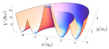
Figure 1: (Color online) The confining potential $V$ of Eq. (1), where $R_{i}=2a_{0}$, $R_{o}=4a_{0}$, and $\omega_{o}/\omega_{i}=5/4$.

In our calculations we consider $R_{i}=2a_{0}$ and $R_{o}=4a_{0}$, where $a_{0}=[\hbar/(M\omega)]^{1/2}$ is the oscillator length corresponding to $\omega=\omega_{i}/4$, and finally $\omega_{o}/\omega_{i}=5/4$. In the outer ring the potential is more tight, $\omega_{o}>\omega_{i}$, in order to compensate for the fact that $R_{o}>R_{i}$, i.e., to make the product of the “width” of each annulus times the radius of each annulus to be comparable to each other. (This is typically also the case in the studies on electrons in quantum rings, in semiconductor heterostructures that we mentioned above.)

To simplify the discussion, we also assume that there is a very tight trapping potential along the $z$ axis (omitted in the potential above), which completely freezes out the degrees of freedom of the gases along this direction. With this assumption, our problem becomes effectively two-dimensional, with the tight dimension entering only implicitly through the parameters $u_{ij}$ in the Hamiltonian of Eq. (2). With the usual assumption of a contact interatomic potential, the Hamiltonian becomes

$$H=\sum_{i=1}^{N_{A}}-\frac{\hbar^{2}}{2M}\nabla_{i}^{2}+V(\rho_{i})+\sum_{j=1}^{N_{B}}-\frac{\hbar^{2}}{2M}\nabla_{j}^{2}+V(\rho_{j})+$$

$$+\frac{u_{AA}}{2}\sum_{i\neq j=1}^{N_{A}}\delta({\bf r}_{i}-{\bf r}_{j})+\frac{u_{BB}}{2}\sum_{i\neq j=1}^{N_{B}}\delta({\bf r}_{i}-{\bf r}_{j})$$

$$+u_{AB}\sum_{i=1,j=1}^{N_{A},N_{B}}\delta({\bf r}_{i}-{\bf r}_{j}).$$ (2)

Here $u_{ij}=(4\pi\hbar^{2}a_{ij}/M)\int|\psi_{0}(z)|^{4}\,dz$, with $\psi_{0}(z)$ being the state of lowest energy of the potential along the $z$ axis and $a_{ij}$ being the $s-$wave scattering lengths for zero-energy elastic atom-atom collisions. The coupled Gross-Pitaevskii-like equations for the order parameters of the two components $\phi_{A}$ and $\phi_{B}$, resulting from the above Hamiltonian, are

$$-\frac{\hbar^{2}\nabla^{2}}{2M}{\phi}_{A}+V(\rho){\phi}_{A}+g_{AA}|{\phi}_{A}|^{2}{\phi}_{A}+g_{AB}|{\phi}_{B}|^{2}{\phi}_{A}$$

$$={\mu}_{A}{\phi}_{A},$$

$$-\frac{\hbar^{2}\nabla^{2}}{2M}{\phi}_{B}+V(\rho){\phi}_{B}+g_{BB}|{\phi}_{B}|^{2}{\phi}_{B}+g_{AB}|{\phi}_{A}|^{2}{\phi}_{B}$$

$$={\mu}_{B}{\phi}_{B}.$$ (3)

In the above equations $\int|{\phi}_{A}|^{2}d{\bf r}=N_{A}/N_{B}$, and $\int|{\phi}_{B}|^{2}d{\bf r}=1$. Also, $g_{AA}=N_{B}u_{AA}$, $g_{BB}=N_{B}u_{BB}$, $g_{AB}=N_{B}u_{AB}$, and $\mu_{i}$ are the chemical potentials. In what follows, we consider repulsive interactions only, $g_{ii}>0$, $g_{ij}>0$, and also assume that $g_{AA}=g_{BB}\equiv g$.

The method that we adopt to solve Eqs. (3) is a fourth-order split-step Fourier method within an imaginary-time propagation approach Chi05 . We start with a reasonable initial state for the two components and propagate it in imaginary time, making sure that we proceed a sufficiently large number of time steps, which guarantee that we have reached a steady state.

III Phase diagram of the ground state

We start with the ground state of the system. There are three energy scales in the problem, namely the single-particle energy that is set by the trap, the intra-atomic interaction energy, and the inter-atomic interaction energy. For weak interactions, the energy is dominated by the single-particle term and the ground state is determined by the minimization of this term. On the other hand, for strong interactions, for a given ratio of the two populations $N_{A}/N_{B}$, the actual symmetry of the ground state results from the competition between the intra-and inter-species coupling strengths; the former favors the maximum possible spread of the two gases within the system, whereas the latter favors the minimization of their spatial overlap.

The most pronounced difference of this problem as compared to the case where there is only one potential minimum – i.e., a single annulus – is the existence of a phase where each component resides in only one of the two potential minima, thus separating radially. In addition, we have also observed the expected azimuthal phase separation when both species occupy the same potential minimum Smy09 ; Ao ; Timm ; PS .

In Fig. 2 we illustrate the phase diagram showing the symmetry of the ground-state density distribution of the two gases as $g_{AB}$ and $g$ are varied, for $N_{A}=N_{B}$. Since $g_{AA}=g_{BB}$ and $N_{A}=N_{B}$, the results are symmetric when the two components are interchanged. The axes in the phase diagram of Fig. 2 may also be considered to represent the values of the scattering lengths $a_{AB}$ and $a_{AA}=a_{BB}$ (scaled appropriately).

We have found three different phases: (i) coexistence of the two species (squares, red color), (ii) azimuthal separation (triangles, blue color), and (iii) radial separation (circles, green color), see Fig. 3. The difference between solid and empty symbols in Fig. 2 refers to the stability of the persistent currents and is explained in the following section.

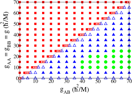
Figure 2: (Color online) Phase diagram in the $g_{AB}$-versus-$g$ plane, which shows the symmetry of the ground-state density distribution of the two components. Squares, triangles and circles correspond to phase coexistence, azimuthal phase separation, and radial phase separation, respectively. The solid (empty) symbols denote points where the currents are metastable (unstable).

As seen in Fig. 2, the phase boundary between phase coexistence and separation of the two components is, to a very good approximation, a straight line given by (setting $\hbar=M=\omega=1$)

$$g_{AB}\approx g+2,$$ (4)

as we have found by fitting numerically our data.

Certain limiting cases in the phase diagram of Fig. 2 may be analyzed and understood easily. In the case $g_{AB}=0$ and $g_{AA}=g_{BB}$, the two gases do not interact with each other. In order to minimize their energy, they distribute homogeneously along the rings and coexist. In the other limiting case $g_{AA}=g_{BB}=0$, for $g_{AB}$ smaller than $\approx 2$, the two components also coexist; however, for larger values than 2, they separate azimuthally. Although in this phase the kinetic energy increases, the interaction energy is lowered due to the repulsion between the two species, and the azimuthal symmetry-breaking persists with increasing $g_{AB}$.

It is also instructive to understand the internal structure of the phase diagram. As one moves vertically, i.e., for a fixed value of $g_{AB}$ (being sufficiently large, such that the components separate azimuthally), for small enough $g$ the two components occupy mainly the inner ring since the repulsion between the particles cannot compensate for the stronger confinement of the outer ring. As $g$ increases, the outer ring becomes progressively more occupied. When the inter-component repulsion $g_{AB}$ becomes large enough, the gases minimize their energy by separating radially. However, if $g$ increases further, the inner ring becomes too small to host one of the species entirely. Azimuthal phase separation takes place again, now with both gases being largely spread within the whole system. Eventually, for even larger values of $g$, the dominant term in the energy is the intra-atomic interaction, and thus the two components coexist.

As anticipated before, we illustrate this effect in Fig. 3, where we plot the densities of the cases with $g_{AB}=55$, and (a) $g=5$, (b) $g=15$, (c) $g=35$, and (d) $g=60$, corresponding to azimuthal phase separation, radial phase separation, azimuthal phase separation, and phase coexistence, respectively.

It is also of interest to investigate the nature of the phase transitions occurring in the system. As one crosses the boundary from coexistence to azimuthal phase separation, the two components decrease continuously their overlap, developing sharper profiles as the repulsion increases. This transition is thus continuous (second order), as it is also the case in purely one-dimensional single rings Smy09 . In the corresponding energy surface, the minimum (which determines the ground state) moves continuously as one crosses the phase boundary. On the contrary, the transitions involving radial separation are discontinuous (first order), indicating that two local minima in the energy surface compete and that the system jumps abruptly from the one state to the other.

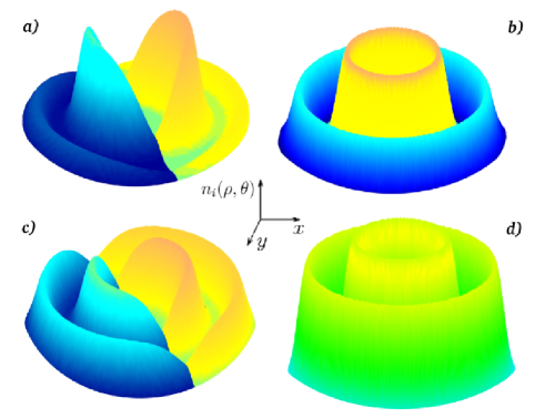
Figure 3: (Color online) Ground-state density distributions $n_{A}(\rho,\theta)=|\phi_{A}(\rho,\theta)|^{2}$ and $n_{B}(\rho,\theta)=|\phi_{B}(\rho,\theta)|^{2}$ of the two components, for $g_{AB}=55$ and (a) $g=5$, (b) $g=15$, (c) $g=35$, and (d) $g=60$, corresponding to azimuthal phase separation, radial phase separation, azimuthal phase separation, and phase coexistence, respectively. The peaks in the densities correspond to the minima of the inner and the outer parabolae of the confining potential.

IV Rotational properties

IV.1 Lowest state of the system for a fixed angular frequency of rotation

The phase transitions that we described above also have a clear influence on the rotational properties of the system. We start by examining the response of the system to some finite rotational frequency $\Omega$ of the trap. In the following we determine the total angular momentum per particle $l=(L_{A}+L_{B})/(N_{A}+N_{B})$ as a function of $\Omega$, $l=l(\Omega)$. Following the usual procedure, we minimize the energy of the system in the rotating frame, i.e., we minimize $E/N-l\Omega$, where $E$ is the total energy. The result of this calculation is shown in Fig. 4, where we have set $N_{A}/N_{B}=1.5$, $g=10$, and $g_{AB}=20$. The typical values of $\Omega$ are rather small because we have scaled it with $\omega_{i}$. However, at least in the case of a purely one-dimensional ring potential, the scale for the typical $\Omega$ is on the order of the frequency $\hbar/(2MR^{2})$ of the corresponding kinetic energy $\hbar^{2}/(2MR^{2})$ Leggett , where $R$ is the radius of the ring. In atomic units, $\hbar=M=\omega=1$, $\omega_{i}=4$, while $\hbar/(2MR^{2})\simeq 1/50$ (for $R$, say, equal to 5). This introduces a factor $10^{-2}$.

It is also instructive to comment on the behavior of the gas as $\Omega$ increases and see the connection of the function $l=l(\Omega)$ with the density distribution of the two components. For $0\leq\Omega/\omega_{i}\leq 0.005$ the two species are separated radially and the total angular momentum is zero. For $\Omega/\omega_{i}\approx 0.005$, the density of the two components breaks its azimuthal symmetry discontinuously, and the angular momentum jumps abruptly to a finite value. Beyond this value of $\Omega/\omega_{i}$ the angular momentum increases linearly with $\Omega$ and is carried by both components, which undergo solid-body rotation. This is an expected result due to the azimuthal symmetry-breaking of the density, as we have confirmed by studying the phases of the two order parameters. When $\Omega/\omega_{i}\approx 0.035$, a new plateau appears, which corresponds to an angular momentum per particle equal to two, and the two species separate radially. As one can see from the plot, there is a sequence between plateaus at integer values of $l$ and straight lines with a positive slope, which are separated by abrupt jumps. This sequence persists up to $\Omega/\omega_{i}\approx 0.085$. Beyond this value of $\Omega$ there is no longer radial separation of the two components due to the large centrifugal force, which forces both gases to occupy the two potential minima and therefore to separate azimuthally.

Similar discontinuous transitions in the function $l=l(\Omega)$ occur in a single-component weakly-interacting Bose-Einstein condensate that rotates in a harmonic trap Rokhsar , and are associated with discontinuous transitions between phases of different symmetries of the single-particle density distribution of the gas. In the present problem, the corresponding different symmetries are the ones where the components separate radially, or azimuthally.

Furthermore, the jumps in the $l=l(\Omega)$ plot are consistent with the fact that for the parameters considered, the system supports persistent currents. In other words, had this function been continuous, then metastability would have not been possible (for a discussion of this effect we refer to Ref. Leggett ).

From the above observations we see that the general picture that emerges by considering a finite rotation of the trap resembles the one where the couplings are varied, with a series of phase transitions between radial and azimuthal separation.

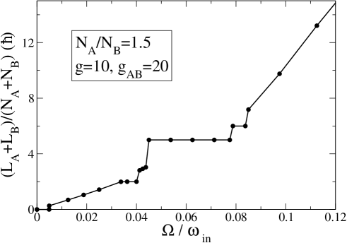
Figure 4: (Color online) The total angular momentum per particle, $(L_{A}+L_{B})/(N_{A}+N_{B})$, as a function of the angular frequency of rotation of the trap $\Omega$, which results from the minimization of the energy in the rotating frame.

IV.2 Metastable currents

Another interesting question is the possible existence of (meta)stable currents. In physical terms, we investigate the energetic (meta)stability of current-carrying states. In the case that there is an energy barrier that separates a current-carrying state from the ground state, in the presence of some dissipative mechanism (such as a thermal cloud, for example) such a state does not decay, and therefore the system supports persistent currents.

We examine two separate aspects of this problem. Firstly, we consider the points of the phase diagram shown in Fig. 2, for a fixed population of the two gases. Secondly, we fix the interaction strengths and vary the ratio $N_{A}/N_{B}$. In both cases we examine the imaginary-time evolution of initial states with some finite, nonzero expectation value of the angular momentum, in the absence of any external rotation of the trap. For a given set of parameters, the existence of a converged final state with a nonzero expectation value of $l$ implies that the associated current is metastable.

IV.2.1 Variable couplings and fixed populations

We have examined all the points that are shown in the phase diagram of Fig. 2. Those corresponding to a final state with a nonzero expectation value of the angular momentum are represented in Fig. 2 with “solid” symbols, while the ones that decay to the non-rotating ground state are represented with “open” symbols.

Clearly, the vast majority of states correspond to metastable currents, except those close to the diagonal $g=g_{AB}$, as well as those with sufficiently small $g$ (for all values of $g_{AB}$). The obtained results show that the angular momentum of the metastable states is always an integer multiple of the particle population, which implies that the associated densities are necessarily circularly symmetric. This is consistent with the statement that circular symmetry is a necessary – though not sufficient – condition for the (meta)stability of the currents, as otherwise the circulation may escape from the gas (since in this case there is no barrier separating the rotating state from the non-rotating one Leggett ).

IV.2.2 Variable relative population and fixed couplings

Let us now study the effect of a variable relative population between the two gases on the (meta)stability of the currents. We thus fix the interaction strengths, as well as the population of the one component $(N_{B})$, and study this question starting from the case with $N_{A}=0$, all the way up to the limit $N_{A}\gg N_{B}$, with an initial state that has some angular momentum in component $B$. Since $N_{B}$ is fixed, the above procedure corresponds physically to keeping the scattering lengths fixed.

As mentioned above, the (meta)stability of the persistent currents depends on the competition between azimuthal phase separation and circular symmetry of the density distribution of the two components. Thus, when $N_{A}=0$, the $B$ component spreads within the whole system for any value of $g$ and the currents can be metastable, provided that the coupling $g$ is sufficiently large. If the population of the component $A$ becomes nonzero but is small enough, it acts only as a weak perturbation, and azimuthal symmetry is still preserved.

However, beyond a critical ratio $N_{A}/N_{B}$, the two species separate azimuthally and the currents are no longer metastable. This critical value depends on the actual intra- and inter-component interaction strengths. A further increase of $N_{A}$ with respect to $N_{B}$ drives the system to a phase of radial separation, and metastability is recovered.

Finally, in the limit where $N_{A}$ becomes too large, this component cannot fit into only one of the two rings. This leads again to azimuthal phase separation of the gases, which is preserved even in the limit $N_{A}\gg N_{B}$. As a result, the stability of the currents is lost again.

We show in Fig. 5 the densities for the case $g=35$, and $g_{AB}=55$ and for various values of the ratio $N_{A}/N_{B}$, in order to illustrate the mentioned sequence of phase transitions. In particular, the results correspond to $N_{A}/N_{B}=0.01$, $N_{A}/N_{B}=0.25$, $N_{A}/N_{B}=0.75$, and $N_{A}/N_{B}=10$, with the first and the third cases corresponding to the metastable states. According to our simulations, changing the values of the interaction strengths modifies the sizes of the “windows” in $N_{A}$ that separate the different phases, but yields qualitatively similar results.

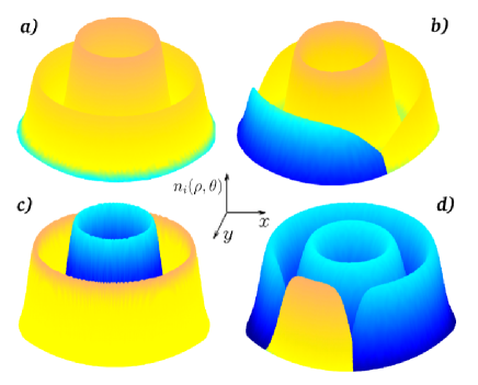
Figure 5: (Color online) Density distributions $n_{A}(\rho,\theta)=|\phi_{A}(\rho,\theta)|^{2}$ and $n_{B}(\rho,\theta)=|\phi_{B}(\rho,\theta)|^{2}$ with $g=35$, and $g_{AB}=55$ of the component $A$ (dark blue) and $B$ (light yellow), for (a) $N_{A}/N_{B}=0.01$, (b) $N_{A}/N_{B}=0.25$, (c) $N_{A}/N_{B}=0.75$, and (d) $N_{A}/N_{B}=10$. In the cases (a) and (c) the states support metastable currents, while in (b) and (d) they do not. The peaks in the densities correspond to the minima of the inner and the outer parabolae of the confining potential.

V Summary and conclusions

As shown in the present study, a coupled system of two distinguishable Bose gases that interact with an effectively-repulsive contact potential and are loaded in a concentric double annular trap reveals a series of phase transitions and the existence of metastable currents.

For weak interactions, when the chemical potential is much smaller than the barrier that separates the two potential minima, the gases are confined in the inner ring, with the width of their transverse profile being smaller than the radius of the ring. Thus, their motion is (at least) close to being quasi-one-dimensional. On the other hand, as the couplings increase, the barrier plays a decreasingly important role, and their transverse width becomes comparable to the radius of the ring(s). Such a trapping potential interpolates up to some extent between one-dimensional and two-dimensional motion, depending on the strength of the coupling between the atoms. The interplay between this effect and the strength of the inter- and intra-atomic couplings gives rise to interesting phase transitions in the ground state of the system, including three different geometries: phase coexistence, radial phase separation, and azimuthal phase separation.

An interesting feature of the system considered is its response to some finite rotational frequency of the trap. The basic picture resembles very much the one where the couplings are varied, inducing axial and/or radial phase separation of the two components.

The robustness in the (meta)stability of the currents that we found for the vast majority of the points in the phase diagram of Fig. 2 is another interesting aspect of this study. Metastability is not found for the cases when the couplings are all nearly equal or exactly equal to each other, as well as for the cases with small $g$, independently of $g_{AB}$.

According to Ref. metastability , a necessary (but not sufficient) condition for metastability is that the trapping potential does not increase monotonically from the center of the trap. The present results suggest that multiple variations in the monotonicity of the trapping potential enhance the stability of the currents.

Last but not least, the discontinuous phase transitions we have found both in the ground-state phase diagram when the two gases separate radially as the couplings are varied, as well as in the response of the system when the rotation of the trap is varied, imply that hysteresis should show up as the coupling/rotational frequency increases/decreases.

VI Acknowledgements

We thank S. Bargi and K. Kärkkäinen for useful discussions. This work was financed by the Swedish Research Council. The collaboration is part of the NordForsk Nordic network “Coherent Quantum Gases - From Cold Atoms to Condensed Matter”.

References

- (1) S. Gupta, K. W. Murch, K. L. Moore, T. P. Purdy, and D. M. Stamper-Kurn, Phys. Rev. Lett. 95, 143201 (2005).
- (2) S. E. Olson, M. L. Terraciano, M. Bashkansky, and F. K. Fatemi, Phys. Rev. A 76, 061404(R) (2007).
- (3) C. Ryu, M. F. Andersen, P. Cladé, V. Natarajan, K. Helmerson, and W. D. Phillips, Phys. Rev. Lett. 99, 260401 (2007).
- (4) K. Henderson, C. Ryu, C. MacCormick, and M. G. Boshier, New J. Phys. 11, 043030 (2009).
- (5) Igor Lesanovsky and Wolf von Klitzing, Phys. Rev. Lett. 99, 083001 (2007).
- (6) Igor Lesanovsky and Wolf von Klitzing, Phys. Rev. Lett. 98, 050401 (2007).
- (7) J. Brand, T. J. Haigh, and U. Zülicke, Phys. Rev. A 80, 011602(R) (2009).
- (8) J. Smyrnakis, S. Bargi, G. M. Kavoulakis, M. Magiropoulos, K. Kärkkäinen, and S. M. Reimann Phys. Rev. Lett. 103, 100404 (2009).
- (9) S. Bargi, J. Christensson, G. M. Kavoulakis, and S. M. Reimann, Phys. Rev. Lett. 98, 130403 (2007).
- (10) J. Christensson, S. Bargi, K. Karkkainen, Y. Yu, G. M. Kavoulakis, M. Manninen, S. M. Reimann, New J. Phys. 10, 033029 (2008).
- (11) P. Ao and S. T. Chui, Phys. Rev. A 58, 4836 (1998).
- (12) E. Timmermans, Phys. Rev. Lett. 81, 5718 (1998).
- (13) C. J. Pethick and H. Smith, Bose-Einstein Condensation in Dilute Gases (Cambridge University Press, Cambridge, England, 2002).
- (14) B. Szafran and F. M. Peeters, Phys. Rev. B 72, 155316 (2005); J. M. Escartín, F. Malet, A. Emperador, and M. Pi, Phys. Rev. B 79, 245317 (2009); T. Mano, T. Kuroda, S. Sanguinetti, T. Ochiai, T. Tateno, J. Kim, T. Noda, M. Kawabe, K. Sakoda, G. Kido, and N. Koguchi, Nanoletters 5, 425 (2005); S. Viefers, P. S. Deo, S. M. Reimann, M. Manninen, and M. Koskinen, Phys. Rev. B 62, 10668 (2000); M. Manninen, M. Koskinen, S. M. Reimann, and B. Mottelson, Eur. Phys. J. D 16, 381.
- (15) S. Viefers, P. Koskinen, P. S. Deo, and M. Manninen, Physica E 21, 1 (2004); S. M. Reimann and M. Manninen, Rev. Mod. Phys. 74, 1283 (2002).
- (16) Similar trap geometries have been considered in coupled quantum rings, see e.g. the first and second papers of CQRs .
- (17) S. A. Chin and E. Krotscheck, Phys. Rev. E 72, 036705 (2005).
- (18) A. J. Leggett, Rev. Mod. Phys. 73, 307 (2001).
- (19) D. A. Butts, and D. S. Rokhsar, Nature (London) 397, 327 (1999).
- (20) K. Kärkkäinen, J. Christensson, G. Reinisch, G. M. Kavoulakis, and S. M. Reimann, Phys. Rev. A 76, 043627 (2007).