An ac field probe for the magnetic ordering of magnets with random anisotropy

Abstract

A Monte Carlo simulation is carried out to investigate the magnetic ordering in magnets with random anisotropy (RA). Our results show peculiar similarities to recent experiments that the real part of ac susceptibility presents two peaks for weak RA and only one for strong RA regardless of glassy critical dynamics manifested for them. We demonstrate that the thermodynamic nature of the low-temperature peak is a ferromagnetic-like dynamic phase transition to quasi-long range order (QLRO) for the former. Our simulation, therefore, is able to be incorporated with the experiments to help clarify the existence of the QLRO theoretically predicted so far.

Over decades, great interest has been intensively addressed to rare-earth magnetic glasses of random magnetic anisotropy (RMA). However, the nature of magnetic phase transition (MPT) and magnetic ordering in such random magnets has still been far from being completely understood ref1 . First, Monte Carlo (MC) simulations were opposite to the prediction of renormalization group theories ref2 ; ref3 to reveal that the second-order MPT exists in three-dimensional weak RMA systems of XY ref4 and Heisenberg spins ref5 ; ref6 . Second, Itakura and Arakawa ref9 have demonstrated that a crucial additional vortex energy should be included in the Imry-Ma type arguments, which have predicted the absence of ferromagnetic long range order (LRO) in magnets of random field (RF) ref7 and RMA ref8 for space dimensions $d<4$, to explain the power-law correlation of quasi-long range order (QLRO) in the Bragg glass state of impure superconductors ref10 , and showed MC results of the power-law scenario for the weak RF model of XY spins. Feldman ref11 has theoretically shown that QLRO can emerge instead of LRO in $d=4-\epsilon$ dimensions and is common in such impure systems of continuous non-Abelian symmetry as magnets of weak RF and RMA. In addition, QLRO has also been clearly evidenced in a number of MC simulations ref5 ; ref9 ; ref12 , of which a power-law spin correlation function has been found to indicate a ground state of QLRO in weak RMA systems of Heisenberg spins ref5 . In spite of these theoretical conjectures, the lack of direct experimental and theoretical agreements in the literature leads to the questions of (i) whether the magnetic transition and low-temperature magnetic order in weak RMA magnets are ferromagnetic-like, and (ii) whether the so-called RMA model ref13 can be applied to understand such phenomena in real materials.

In this Letter, we address these questions by conducting a MC simulation upon the RMA model ref13 . Our simulation aims to clarify an experimental possibility that the singularity on the temperature-dependent curves of the real part of the ac susceptibility, $\chi^{\prime}(T,\omega)$, for a weak RMA glass of a-Ho₂₈Fe₇₂ amorphous film reported by Saito et al. ref14 manifests a second-order MPT, which is discriminated in nature from the magnetic glassy phase transition (GPT) in strong RMA glasses, for instance, Dy₄₀Al₂₄Co₂₀Y₁₁Zr₅ bulk glass ref15 . Differing from the MPT, the GPT is indicated by a glassy critical slowing down law without any singularity shown on $\chi^{\prime}(T,\omega)$ at the transition temperature, $T_{\rm g}$ ref15 . Notice that a similar scenario, but for a case of RF systems, has been existed in the literature when Schremmer and Kleemann ref16 demonstrated for an orientational glass system of K_1-xLi_xTaO₃ with $x=0.063$ (a doping well above the glassy and ferroelectric boundary $x_{\rm c}\sim 0.022$) that the singularity on the real part of the ac dielectric permittivity, $\epsilon^{\prime}(T,\omega)$, is of a transition to the long-range ferroelectric phase. However, this is a first-order transition.

In the light of these experiments, we show in the present work that the nature of the aforementioned singularity for the weak RMA magnet of a-Ho₂₈Fe₇₂ amorphous film ref14 can be understood dynamically with the concept of dynamic transition within the framework of the RMA model of three-dimensional Heisenberg spins ref13 , of which the Hamiltonian can be written as

$$\mathcal{H}=-J\sum_{\langle i,j\rangle}{\vec{S}_{i}\cdot\vec{S}_{j}}-D\sum_{i}{(\hat{a}_{i}\cdot\vec{S}_{i})^{2}}-H\sum_{i}{\vec{S}_{i}\cdot\hat{z}},$$ (1)

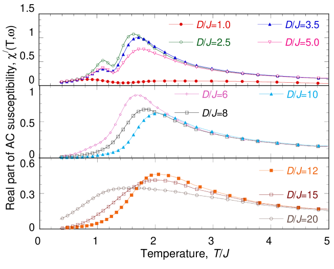
Figure 1: $\chi^{\prime}(T,\omega)$ curves at $\omega=3\times 10^{-3}$ and $H_{0}=0.05$ for various $D/J$ values. $\chi^{\prime}(T,\omega)$ exhibits distinct characteristics of weak ($D/J\leq 5$) and strong ($D/J>5$) degrees of RMA.

where the first term is due to the exchange coupling with strength $J>0$ between nearest-neighbor spins, the second is for on-site RMA with strength $D>0$, and the last is the Zeeman term with the presence of an external field of strength $H$ along $\hat{z}$ axis. $\vec{S}_{i}$ and $\hat{a}_{i}$ are unit vectors representing the spin (an annealed variable) and the random easy axis (a randomly-quenched variable) at site $i$, respectively. In Eq. (1), the anisotropy to exchange ratio, $D/J$, plays the role of the degree of RMA. One prominent effect of the degree of RMA is clearly observed in Fig. 1. Here, $\chi^{\prime}(T,\omega)$ is simulated using the same MC technique as that described in our previous papers ref17 ; ref18 for simple-cubic-lattice systems of $L\times L\times L$ ($L=10$) Heisenberg spins as an external ac field, $H=H_{0}\sin(\omega t)$, is applied, where $H_{0}/J=0.05$, time $t$ is in MC step (MCS), and frequency $\omega$ is in MCS^-1. Each data point is averaged over $50$ realizations of {$\hat{a}_{i}$}${}^{L^{3}}_{1}$. As shown in Fig. 1, curves of $\chi^{\prime}(T,\omega)$ with $\omega=3\times 10^{-3}$ exhibit two peaks for small values of $D/J$, i.e., weak RMA ($D/J\leq 5$). The high-temperature peak is responsible for an Arrhenius-type relaxation which is in common with that for those curves of large values of $D/J$ of strong RMA, whereas the low-temperature peak peculiarly characterizes another magnetic nature of magnets of weak RMA, the position of which is almost insensitive to the change of anisotropy strength. Notice that in our simulation, we mimic the measurement protocol that the system is cooled in the ac field to the lowest temperature then carrying out the calculation of ac susceptibility and other quantities when heating the system up. The reason for this choice is because we have seen in our simulation that, unlike the RF system of K_1-xLi_xTaO₃ with $x=0.063$ ref16 , cooling the systems of weak RMA in a nonzero dc field even as small as $H_{0}$ shall unexpectedly result in the suppression of the low-temperature peak of $\chi^{\prime}(T,\omega)$ curve and the curve looks like that of strong RMA, i.e., an one-peak curve. Interestingly, these distinct characteristics of $\chi^{\prime}(T,\omega)$ for weak and strong RMA systems are consistent with results reported by Itakura ref5 that the function $G(r)\propto r^{-\eta-1}\exp(-r/\xi)$ can be used to describe spin correlation of the ground state for the RMA model in Eq. (1). The correlation length $\xi$ is finite for large values of $D/J$ while it is infinite for weak RMA of $D/J\leq 5$ so that the spin correlation reduces to a frozen power law of QLRO ground state, $G(r)\propto r^{-\eta-1}$. We remark that we shall only focus on a weak RMA glass of $D/J=3.5$ and a strong RMA glass of $D/J=10$ which are typical of the RMA model of Heisenberg spins in Eq. (1) to understand magnetic behaviors of weak RMA a-Ho₂₈Fe₇₂ ref14 and strong RMA Dy₄₀Al₂₄Co₂₀Y₁₁Zr₅ glasses ref15 , respectively.

Figure 2 presents the temperature dependence of $\chi^{\prime}(T,\omega)$ at different frequencies and $H_{0}/J=0.05$ for $D/J=3.5$ and $D/J=10$ cases. For $D/J=3.5$, curves of $\chi^{\prime}(T,\omega)$ exhibit two peaks. The position of the low-temperature one, $T_{\rm{p}}$, is insensitive to frequency and is at about $T_{\rm p}/J\approx 1.15$. The position of the high-temperature one, $T_{\rm b}(\omega)$, shifts toward low temperature in an Arrhenius way with decreasing frequency in addition to increasing the heights of the two peaks. At sufficient low frequencies, in this case $\omega\leq 5\times 10^{-4}$, the two peaks merge together so that $\chi^{\prime}(T,\omega)$ rockets up then drops abruptly at about $T_{\rm c}/J=1.0$. This fashion is what has been experimentally shown for the a-Ho₂₈Fe₇₂ glass and the “dip” in $\chi^{\prime}(T,\omega)$, which occurs at the same position of the single peak in $\chi^{\prime\prime}(T,\omega)$ (not shown), indicates a signature of the MPT singularity ref14 . Besides, the temperature dependence of the ac susceptibility obtained in our MC simulations for the $D/J=3.5$ case also shows another feature resembling the experiment of a-Ho₂₈Fe₇₂ glass. In contrast to spin glasses (SGs), $\chi^{\prime\prime}(\omega)>\chi^{\prime}(\omega)$ in the vicinity of the singularity, which, according to Saito et al. ref14 , “implies that the center $\tau_{\rm c}$ of distribution of relaxation time $g(\ln\tau)$ is much longer than the measuring time constant $t=1/\omega$.” Focussing on the dynamic behavior at the transition region, the authors applied a phenomenological Cole-Cole model of polydispersive relaxation which yields the ac susceptibility as $\chi(\omega)=\chi_{\rm{a}}+(\chi_{0}-\chi_{\rm{a}})/\{t1+(i\omega\tau_{\rm c})^{\beta}\}$ and $g(\ln\tau)=\sin(\beta\pi)/2\pi\{\cosh[\beta\ln(\tau/\tau_{\rm{c}})]+\cos(\beta\pi)\}$, where $\chi_{0}$ and $\chi_{\rm{a}}$ are static and high frequency limit susceptibilities, and $0<\beta<1$. They found that $g(\ln\tau)$ is almost Gaussian in $\ln\tau$ and symmetric about $\ln\tau_{\rm c}$, $\beta$ reduces from $1$ to $0.4$ and $\tau_{\rm{c}}$ becomes longer and longer with decreasing temperature toward $T_{\rm{c}}$ in company with broadening of $g(\ln\tau)$. All of these features are similar to SGs, however, $\tau_{\rm{c}}$ for the a-Ho₂₈Fe₇₂ glass is several orders of magnitude longer than those of SGs. On the other hand, the low-temperature peak is suppressed for all frequencies in the $D/J=10$ case like that of strong RMA of Dy₄₀Al₂₄Co₂₀Y₁₁Zr₅ glasses ref14 ; ref15 . Nonetheless, we did find that there is a well-determined transition temperature, $T_{\rm g}$, of the GPT for both $D/J=3.5$ and $D/J=10$ cases by means of the scaling law of critical slowing-down dynamics, $\tau_{\rm c}=\tau^{\ast}[T_{\rm b}(\omega))/T_{\rm g}-1]^{-z\nu}$, shown in the insets of Fig. 2. In terms of this scaling law, the magnetic glassy behaviors for systems of weak and strong RMA are expected to be the same and like those of SGs ref11 . For instance, if the critical exponent $\nu$ of the correlation length roughly takes values in the range of $0.7\sim 0.8$ ref4 ; ref6 then the dynamical exponent $z$ may be $1.85\sim 2.35$, i.e., consistent with the magnitude of those for SGs ref19 . Another example is that Billoni et al. ref20 have reported aging phenomena for the $D/J=3.5$ case similar to those of Heisenberg SGs at low temperatures. To this end, a question remaining unsolved is what is the nature of the low-temperature peak in $\chi^{\prime}(T,\omega)$ for the $D/J=3.5$ case, which will be cleared up as below.

Figs. 3 and 4 present the results of the temperature dependence of $m_{z}(T,\omega)$, $\chi_{z}(T,\omega)$, and $\chi^{\prime}(T,\omega)$ from which one can see clearly evidences of MPT for the $D/J=3.5$ case but not for the $D/J=10$ case. $m_{z}(T,\omega)$ is the averaged magnetization per spin projected along $z$ direction, and $\chi_{z}(T,\omega)$ is the thermodynamic fluctuation of the magnetization. In Fig. 3, curves of $m_{z}(T,\omega)$ are shown for these two cases with frequencies $1\times 10^{-4}\leq\omega\leq 1\times 10^{-2}$ and $H_{0}/J=0.05$. For the sake of reference, one curve of $m_{z}(T,\omega)$ at $\omega=1\times 10^{-4}$ (i.e., the violet-colored solid line) is also plotted for $D/J=0$, the case of non-anisotropic pure Heisenberg model possessing a well-known ferromagnetic phase transition ref21 . For $D/J=3.5$, the transition width of magnetization does not change until low frequencies $\omega\leq 5\times 10^{-4}$ with which the width gets narrower and narrower and $m_{z}(T,\omega)$ curve approaches to the curve for $D/J=0$. This change apparently corresponds to the change of the low-temperature peak with frequency in $\chi^{\prime}(T,\omega)$ shown in Fig. 2. Strikingly, $\chi_{z}(T,\omega)$ in the inset of Fig. 3 exhibits a sharp peak similar to that of the $D/J=0$ case, i.e., a ferromagnetic-like MPT. This result supports the coexistence of MPT and GPT revealed for the case $D/J=4$ of the RMA model in Eq. (1) ref5 . In contrast, the transition in magnetization of the $D/J=10$ case is quite broad. This is indicated further in the inset of Fig. 3 by the noisy blurring peak of $\chi_{z}(T,\omega)$ whose height is orders of magnitude lower than those of $D/J=3.5$ and $D/J=0$ cases. In addition, the magnetization at low temperatures for the $D/J=3.5$ case is high in magnitude of 0.7, albeit smaller than 1.0 for the $D/J=0$ case, and frequency-independent against the small and chaotically frequency-dependent value of that for the $D/J=10$ case. This feature is probably due to their different magnetic structures: the asperomagnet (known in literature as a correlated spin-glass or a “ferromagnet” with wandering axis) in the former versus the speromagnet in the latter ref1 ; ref22 . We believe that MPT for $D/J=10$ likely does not exist or at least is smeared out by strong RMA and this is why the low-temperature peak is suppressed completely in $\chi^{\prime}(T,\omega)$ curves.

In general, a phase transition like those for the $D/J=0$ and $D/J=3.5$ cases has been termed the dynamic transition, which is a true thermodynamic phase transition usually studied together with the dynamic hysteresis in pure magnetic systems (the systems without any random defect or anisotropy to pin the magnetic domains) ref23 ; ref24 . These phenomena occur due to a relaxational delay of the magnetization in response to the, say, oscillating field. When the oscillation period of the field is much less than the effective relaxation time of the magnetic system the hysteresis loop becomes asymmetric about the origin with a nonvanishing area and a “spontaneously broken symmetric phase” arises dynamically with a nonvanishing value of the dynamic order parameter $Q$, defined as $Q(T,\omega)=(\omega/2\pi)\oint m(T,t)dt$ ($Q(T,\omega)$ is the period averaged magnetization and is equal to $m_{z}(T,\omega)$ in our notation), where the instantaneous magnetization per site at time $t$ and temperature $T$ is calculated as $m(T,t)=(1/L^{3})\sum_{i}\vec{S}_{i}(T,t)\cdot\hat{z}$. The system is in a dynamically-ordered phase when $Q\neq 0$ and the loop is asymmetric or in a dynamically-disordered phase when $Q=0$ and the loop is symmetric. A transition occurs at $T_{d}$ when one crosses the boundary separating the two phases. Notice that the boundary is dynamic in nature since $T_{d}$ depends on both $H_{0}$ and $\omega$, i.e., $T_{d}=T_{d}(H_{0},\omega)$. For any fixed frequency, the $H_{0}-T$ plane is then divided by the dynamic phase boundary line $T_{d}(H_{0},\omega)$, which is in general convex towards the origin. With large values of $H_{0}$, one gets a “forced oscillation” kind of scenario inducing the dynamically-disordered phase ($Q=0$) at high $T$ that gives rise to low values of $T_{d}(H_{0},\omega)$. All of these features of the phase diagram have been obtained for pure magnetic systems of Ising models using mean-field and MC methods ref24 . They are also observed in our MC simulation for the weak RMA Heisenberg model as shown in Fig. 4 for the $D/J=3.5$ case with $H_{0}/J=0.05\sim 2.5$ and $\omega=3\times 10^{-3}$. Very interestingly, the dip in $\chi^{\prime}(T,\omega)$ as well as the only peak in $\chi^{\prime\prime}(T,\omega)$ occur somewhere around $T_{d}(H_{0},\omega)$ and quite similar to the fashion for two- and three-dimensional pure Ising models ref24 . (note, however, that it is difficult to determine $T_{d}(H_{0},\omega)$ in the $m_{z}(T,\omega)$ (i.e., $Q(T,\omega)$) curve because $m_{z}(T,\omega)$ undergoes a gradually broad transition shown in Fig. 4. Instead, we prefer to take the temperature $T_{a}$ at the peak in $\chi_{z}(T,\omega)$ or equivalently the temperature $T_{p}$ at the low-temperature peak in $\chi^{\prime}(T,\omega)$ to construct the diagram of the dynamic transition for the $D/J=3.5$ case shown in the inset of Fig. 4.) Eventually, in ac susceptibility measurements one may be indicated precisely the same dynamic transition (where the peaks or dips are shown) as that the dynamic order parameter (if it could be directly measured in experiment) provides as long as the values of $H_{0}$ are very small so that the dynamic transition is continuous because large values of $H_{0}$ lead to a crossover of continuous/discontinuous transition at the tricritical point (not shown in our simulation) in the $H_{0}-T$ diagram ref23 ; ref24 . Therefore, the ac susceptibility for a-Ho₂₈Fe₇₂ ref14 is a particularly prominent example to study experimentally the dynamic transition in weak RMA systems using the ac susceptibility measurements.

In summary, our MC simulation shows that the RMA model in Eq. (1) can be employed to understand the distinct behaviors in $\chi^{\prime}(T,\omega)$ of a-Ho₂₈Fe₇₂ and Dy₄₀Al₂₄Co₂₀Y₁₁Zr₅ glasses ref14 ; ref15 where the nature of the low-temperature peak of $\chi^{\prime}(T,\omega)$ for the former is a dynamic transition. This result marks a striking similarity between weak RMA Heisenberg model and pure ferromagnetic spin models and sheds light on the nature of magnetic transition and magnetic ordering, i.e., QLRO, in magnets with weak random anisotropy.

This work was financially supported by the National Science Council of Taiwan, R.O.C, under Grant No. NSC 97-2112-M-007-007-MY3.

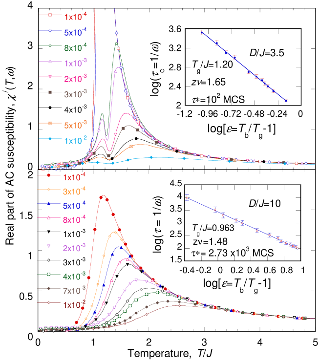
Figure 2: Temperature dependence of $\chi^{\prime}(T,\omega)$ at various frequencies and $H_{0}=0.05$ for $D/J=3.5$ (upper panel) and $D/J=10$ (lower panel). Insets show laws of critical slowing-down dynamics for the two cases, respectively.

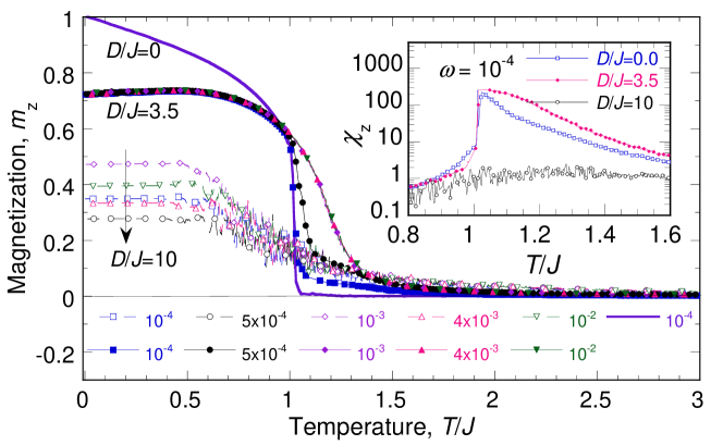
Figure 3: Temperature dependence of $m_{z}(T,\omega)$ at various frequencies and $H_{0}=0.05$ for $D/J=0$ (solid line), $D/J=3.5$ (solid symbols), and $D/J=10$ (open symbols). The inset shows $\chi_{z}(T,\omega)$ for these cases at $\omega=1\times 10^{-4}$.

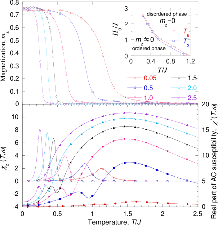
Figure 4: Temperature dependence of $m_{z}(T,\omega)$, $\chi_{z}(T,\omega)$, and $\chi^{\prime}(T,\omega)$ for $D/J=3.5$ at $\omega=3\times 10^{-3}$ and different values of $H_{0}$ (different colored curves). The one-peak and two-peak curves are $\chi_{z}(T,\omega)$ and $\chi^{\prime}(T,\omega)$, respectively. The inset presents the dynamic phase diagram in $H_{0}-T$ plane, where the $T_{\rm a}$ line (or the $T_{\rm p}$ line) shows the dynamic phase boundary between the dynamically-ordered phase ($m_{z}\neq 0$) and dynamically-disordered phase ($m_{z}=0$).

References

- (1) K. Moorjani and J. M. D. Coey, Magnetic Glasses, (Elsevier, New York, 1984); D. H. Ryan edt, Recent Progress in Random Magnets, (World Scientific, Singapore, 1992); R. W. Cochrane, R. Harris, and M. J. Zuckermann, Phys. Reports 48, 1 (1978).
- (2) Y. Holovatch, V. Blavatoska, M. Dudka, C. Von Ferber, R. Folk, and T. Yavorsokii, Inter. J. Mod. Phys. B 16, 4027 (2002); M. Dudka, R. Folk, and Y. Holovatch, J. Magn. Magn. Mater. 294, 305 (2005); M. Dudka, R. Folk, Y. Holovatch, and G. Moser, J. Phys. A 40, 8247 (2007).
- (3) A. Aharony, Phys. Rev. B 12, 1038 (1975).
- (4) U. K. Rößler, Phys. Rev. B 59, 13577 (1999); R. Fisch, Phys. Rev. B 79, 214429 (2009).
- (5) M. Itakura, Phys. Rev. B 68, 100405 (2003).
- (6) Ha M. Nguyen and P. Y. Hsiao, J. Appl. Phys. 105, 07E125 (2009).
- (7) Y. Imry and S. Ma, Phys. Rev. Lett. 35, 1399 (1975).
- (8) R. A. Pelcovits, E. Pytte, and J. Rudnick, Phys. Rev. Lett. 40, 476 (1978).
- (9) M. Itakura and C. Arakawa, Prog. Theor. Phys. Suppl. 157, 136 (2005).
- (10) N. Avraham., B. Khaykovich, Y. Myasoedov, M. Rappaport, H. Shtrikman, Di. E. Feldman, T. Tamegai, P. H. Kesk, M. Lik, M. Konczykowski, K. van der Beek, and E. Zeldov, Nature 411, 451 (2001); F. F. Bouquet, C. Marcenat, E. Steep, R. Calemczuk, W. K. Kwok, U. Welp, G. W. Crabtree, R. A. Fisher, N. E. Phillips, and A. Schilling, Nature 411, 448 (2001).
- (11) D. E. Feldman, Phys. Rev. B 61, 382 (2000); Phys. Rev. Lett. 84, 4886 (2000).
- (12) R. Fisch, Phys. Rev. B 39, 873 (1989); Phys. Rev. B 42, 540 (1990); Phys. Rev. B 62, 361 (2000); Phys. Rev. Lett. 66, 2041 (1991).
- (13) R. Harris, M. Plischke, and M. J. Zuckermann, Phys. Rev. Lett. 31, 160 (1973).
- (14) T. Saito, A. Suto, and S. Takenaka, J. Magn. Magn. Mater. 272-276, 1319 (2004).
- (15) Q. Luo, D. Q. Zhao, M. X. Pan, and W. H. Wang, Appl. Phys. Lett. 92, 011923 (2008).
- (16) H. Schremmer and W. Kleemann, Phys. Rev. Lett. 62, 1896 (1989).
- (17) Ha M. Nguyen and P. Y. Hsiao, J. Korean Phys. Soc. 53, 2447 (2008).
- (18) Ha M. Nguyen and P. Y. Hsiao, Appl. Phys. Lett. 94, 186101 (2009).
- (19) K. Binder and A. P. Young, Rev. Mod. Phys. 58, 801 (1986).
- (20) O. V. Billoni, S. A. Cannas, and F. A. Tamarit, Phys. Rev. B 72, 104407 (2005).
- (21) D. P. Landau and K. Binder, A Guide to Monte Carlo Simulations in Statistical Physics, (Cambridge Press, Cambridge, Second Edition, 2005).
- (22) E. M. Chudnovsky and R. A. Serota, Phys. Rev. B 26, 2697 (1982); J. M. D. Coey, J. Appl. Phys. 49, 1646 (1978).
- (23) B. K. Chakrabarti and M. Acharyya, Rev. Mod. Phys. 71, 847 (1999).
- (24) M. Acharyya and B. K. Chakrabarti, Phys. Rev. B 52, 6550 (1995).