The X-ray luminous cluster underlying the bright radio-quiet quasar H1821+643

Abstract

We present a Chandra observation of the only low redshift, $z=0.299$, galaxy cluster to contain a highly luminous radio-quiet quasar, H1821+643. By simulating the quasar PSF, we subtract the quasar contribution from the cluster core and determine the physical properties of the cluster gas down to $3\arcsec$ ($15\rm\thinspace kpc$) from the point source. The temperature of the cluster gas decreases from $9.0\pm 0.5\rm\thinspace keV$ down to $1.3\pm 0.2\rm\thinspace keV$ in the centre, with a short central radiative cooling time of $1.0\pm 0.1\rm\thinspace Gyr$, typical of a strong cool-core cluster. The X-ray morphology in the central $100\rm\thinspace kpc$ shows extended spurs of emission from the core, a small radio cavity and a weak shock or cold front forming a semi-circular edge at $\sim 15\arcsec$ radius. The quasar bolometric luminosity was estimated to be $\sim 2\times 10^{47}\hbox{$\rm\thinspace erg\rm\thinspace s^{-1}\,$}$, requiring a mass accretion rate of $\sim 40\hbox{$\hbox{$\rm\thinspace M_{\odot}$}\rm\thinspace yr^{-1}\,$}$, which corresponds to half the Eddington accretion rate. We explore possible accretion mechanisms for this object and determine that Bondi accretion, when boosted by Compton cooling of the accretion material, could provide a significant source of the fuel for this outburst. We consider H1821+643 in the context of a unified AGN accretion model and, by comparing H1821+643 with a sample of galaxy clusters, we show that the quasar has not significantly affected the large-scale cluster gas properties.

1 Introduction

The central radiative cooling time of the Intracluster Medium (ICM) in nearby galaxy clusters can drop below $1\rm\thinspace Gyr$ and without a compensating source of heat the gas would rapidly cool down to low temperatures (for a review see Fabian 1994). However, the large reservoir of cool gas implied by this cooling flow model exceeds the amount of molecular gas observed (eg. Edge & Frayer 2003), and the inferred star formation rates by an order of magnitude (Johnstone et al. 1987; Hicks & Mushotzky 2005; Rafferty et al. 2006; O’Dea et al. 2008). In addition, recent high resolution X-ray spectroscopy has been unable to find the emission signatures of gas cooling below about $1\rm\thinspace keV$ at the extreme rates predicted by the cooling flow model in the absence of heating (Peterson et al. 2003; Kaastra et al. 2004; Peterson & Fabian 2006). A heating mechanism is therefore required to stabilise the cooling in cluster cores (for a review see McNamara & Nulsen 2007).

High resolution images of nearby cluster cores taken by the Chandra X-ray Observatory have revealed complex structures, such as cavities, shock fronts and ripples, which have been produced by the central AGN (eg. Boehringer et al. 1993; Fabian et al. 2000, 2003, 2006; McNamara et al. 2000, 2001; Schindler et al. 2001; Forman et al. 2005; McNamara & Nulsen 2007). X-ray cavities, or bubbles, expanded into the ICM by the AGN provide a direct and relatively reliable means of measuring the mechanical energy injected by the SMBH (eg. Jones & De Young 2005). In this way, AGN heating has been shown to be energetically capable of balancing the cooling losses in cluster cores (Bîrzan et al. 2004; Rafferty et al. 2006; Dunn & Fabian 2006; McNamara et al. 2006). Repeated cycles of AGN mechanical heating could support the cluster gas in a relatively stable state.

The galaxy cluster surrounding the quasar H1821+643, at redshift $z=0.299$, was discovered optically by Schneider et al. (1992) and later detected in X-rays by Hall et al. (1997) and Saxton et al. (1997). The cluster is optically rich with an Abell richness class $>2$ (Lacy et al. 1992). The quasar’s radio luminosity at $5\rm\thinspace GHz$ lies in the classification for ‘radio-quiet’ quasars (at only $10^{23.9}\hbox{$\rm\thinspace W\hbox{$\rm\thinspace Hz^{-1}\,$}\hbox{$\rm\thinspace sr^{-1}\,$}\,$}$) and its $151\rm\thinspace MHz$ radio luminosity, which is $10^{25.3}\hbox{$\rm\thinspace W\hbox{$\rm\thinspace Hz^{-1}\,$}\hbox{$\rm\thinspace sr^{-1}\,$}\,$}$ (Blundell & Rawlings 2001), is at the boundary observed to separate FR I and FR II structures. A deep VLA radio image of H1821+643 revealed that, although classified as a radio-quiet quasar, H1821+643 hosts a giant $300\rm\thinspace kpc$ FR I radio source (Blundell & Rawlings 2001). H1821+643 has previously been observed several times with the Chandra X-ray Observatory but in all cases with the gratings in place (HETG Fang et al. 2002, LETG Mathur et al. 2003) which have prevented a detailed analysis of the cluster emission. Fang et al. (2002) were able obtain a spectrum of the cluster from the zeroth-order observation and found a temperature of $\sim 10\rm\thinspace keV$ and a metal abundance of $0.3\hbox{$\thinspace\mathrm{Z}_{\odot}$}$.

In this work, we present new Chandra observations of H1821+643 without the gratings which have allowed us to analyse the underlying ICM and the interactions with the powerful central quasar. By comparing our results with a sample of nearby cool core clusters, we have explored the implications of two different modes of AGN feedback for H1821+643 and investigated the impact this would have on the evolution of the ICM.

We assume $H_{0}=70\hbox{$\hbox{$\rm\thinspace km\rm\thinspace s^{-1}\,$}\rm\thinspace Mpc^{-1}\,$}$, $\Omega_{m}=0.3$ and $\Omega_{\Lambda}=0.7$, translating to a scale of $4.4\rm\thinspace kpc$ per arcsec at the redshift $z=0.299$ of H1821+643. All errors are $1\sigma$ unless otherwise noted.

2 Data Preparation

H1821+643 was observed by Chandra for a total of $90\rm\thinspace ks$ split into four separate observations taken over nine days with the ACIS-S instrument (Observation IDs: 9398 $34\rm\thinspace ks$, 9845 $25\rm\thinspace ks$, 9846 $18\rm\thinspace ks$ and 9848 $11\rm\thinspace ks$). The data were analysed using CIAO version 4.1.2 with CALDB version 4.1.2 provided by the Chandra X-ray Center (CXC). The level 1 event files were reprocessed to apply the latest gain and charge transfer inefficiency correction and then filtered for bad grades to remove cosmic ray events. For this analysis, the improved background screening provided by VFAINT mode was not applied. In the pileup affected region some of the real X-ray events would be marked as background events and excluded by the VFAINT filter leaving a hole in the quasar surface brightness. To filter the datasets for periods affected by flares we examined the ACIS-S1 chip, which did not contain any extended cluster emission. The background lightcurve for this chip was filtered using the lc_clean script provided by M. Markevitch and the $\sim 4\rm\thinspace ks$ affected by flares were then excluded from the ACIS-S3 level 2 event files. The final cleaned exposure time was $85\rm\thinspace ks$.

As the four separate observations were taken so closely together, with effectively identical chip positions and roll angles, we were able to reproject them to a common position (Obs ID: 9398) and combine them. An exposure-corrected image combining the four final cleaned event files is shown in Fig. 1. The exposure map assumed a monoenergetic distribution of source photons of $1.5\rm\thinspace keV$, which is approximately the peak energy of the source. Assuming that all X-ray counts within 3″radius of the point source were from the quasar and all counts external to that were from the cluster, we estimate there to be $\sim 100,000$ cluster counts and $\sim 15,000$ quasar counts, although the latter will have been significantly reduced by pileup.

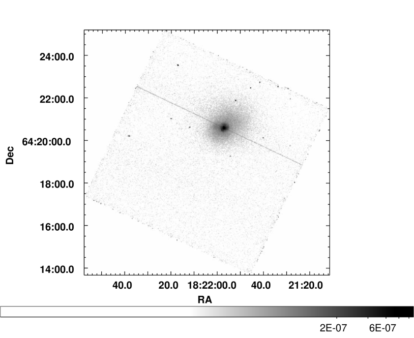
Figure 1: Exposure-corrected image of the ACIS-S3 chip in the 0.5–7.0$\rm\thinspace keV$ energy band smoothed with a 2D Gaussian $\sigma=1.5\arcsec$. The logarithmic scale bar has units $\rm\thinspace photons\rm\thinspace cm^{-2}\rm\thinspace s^{-1}\rm\thinspace pixel^{-1}\,$. The straight line running across the entire image through the centre of the quasar is the readout streak, an instrumental artifact produced by the bright quasar.

2.1 Pileup

Pileup occurs whenever two or more photons, arriving in the same detector region and within a single ACIS frame integration time, are detected as a single event (see eg. Davis 2001). This effect hardens the source spectrum, because photon energies sum to create a detected event of higher energy, and causes grade migration. All events detected by ACIS are graded based on the shape of their charge cloud distributions in a $3\times 3$ pixel island. This grade is used to distinguish between a real photon or a background event, such as a cosmic ray. However, pileup modifies the distribution of charge and therefore alters the event grade.

Following the CXC analysis of the Chandra PSF, the extent of pileup in the observation was estimated using the ratio of “good” grades (grades 0,2,3,4,6) to “bad” grades (grades 1,5,7) defined with observations from the ASCA satellite. The bad/good ratio is shown as a function of radius in Fig. 2 for two energy bands. The ratio was determined in circular annuli which scale logarithmically in width to produce approximately the same number of source counts in each radial bin.

Most of the emission from the quasar comes from the $0.5-2.0\rm\thinspace keV$ energy band which, when piled up, was detected as higher energy photons above $2\rm\thinspace keV$. The $2.0-5.0\rm\thinspace keV$ energy band was therefore used to estimate the radial extent of pileup for this observation. Fig. 2 shows that pileup rapidly increases inside $3^{\prime\prime}$ and dominates at $1^{\prime\prime}$. The rise in the bad/good ratio beyond $\sim 50^{\prime\prime}$ is caused by the increasing importance of the particle background. To minimise the effects of pileup, the region inside $3^{\prime\prime}$ was excluded from our analysis. This choice was also later confirmed to be appropriate by repeating the marx simulation of the quasar with pileup (Appendix A2).

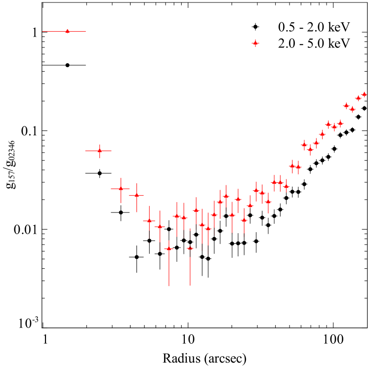
Figure 2: Ratio of ASCA bad grades (g₁₅₇) to ASCA good grades (g₀₂₃₄₆) for H1821+643 in two energy bands.

3 Imaging Analysis

In Fig. 3 we show a merged exposure-corrected image of H1821+643 centred on the bright, piled up quasar, with superimposed $1.4\rm\thinspace GHz$ radio contours from Blundell & Rawlings (2001). The extended cluster emission surrounding the quasar is elongated in a north-west to south-east direction. A surface brightness edge is also visible around the cluster core at a radius of approximately $15\arcsec$ from the quasar. The edge, possibly indicative of a shock in the cluster gas, is most sharply defined around the north-west of the cluster core.

The unsharp-masked image (Fig. 4 centre) highlights the edge in the surface brightness which can be seen to run round the cluster core from the north-west to south-east. This does not appear to be a symmetrical feature about the quasar; the radius of the edge varies from $13\arcsec$ to $17\arcsec$. Although the X-ray emission is extended to the north and south, there does not seem to be a close association with the $1.4\rm\thinspace GHz$ radio emission. The fractional difference image (Fig. 4 right) shows a bright extended spur of emission to the south-east of the AGN containing a surface brightness depression which could indicate a cavity. This X-ray depression is coincident with the inner part of the radio lobes but there is no close correlation with the outer region of the radio emission. Projection effects may have prevented a clean interpretation of the relation between X-ray and radio emission.

There are potentially three additional cavities in the X-ray emission (north-west, north-east and south-west of the quasar, Fig. 4 right). However, these are not coincident with any $1.4\rm\thinspace GHz$ radio emission and it is not clear how they could have reached their current locations.

To more quantitatively investigate the interaction between the quasar and the cluster, we extracted the properties of the cluster gas as close in to the quasar as possible.

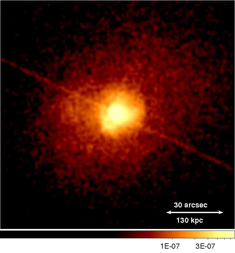
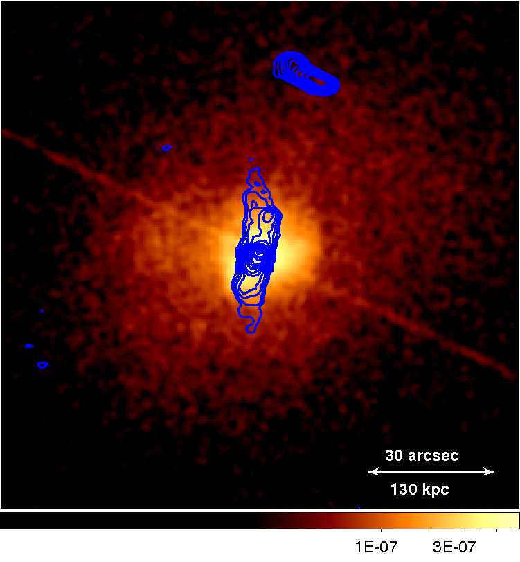
Figure 3: Left: Exposure-corrected image in the 0.5–7.0$\rm\thinspace keV$ energy band smoothed with a 2D Gaussian $\sigma=1.5\arcsec$. The logarithmic scale bar has units $\rm\thinspace photons\rm\thinspace cm^{-2}\rm\thinspace s^{-1}\rm\thinspace pixel^{-1}\,$. Right: with superimposed VLA $1.4\rm\thinspace GHz$ radio contours from Blundell & Rawlings (2001).

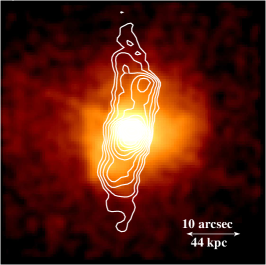
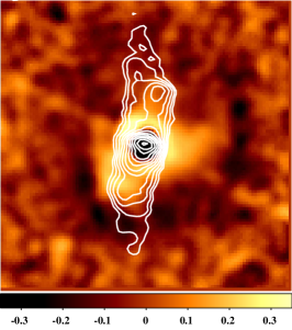
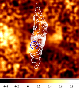
Figure 4: Images of the central $0.8\times 0.8\arcmin$ with superimposed VLA $1.4\rm\thinspace GHz$ radio contours from Blundell & Rawlings (2001). Left: Exposure-corrected image in the 0.5–7.0$\rm\thinspace keV$ energy band smoothed with a 2D Gaussian $\sigma=1.5\arcsec$. Centre: Unsharp-masked image, created by subtracting images smoothed by 2D Gaussians with $\sigma=1$ and $5\arcsec$ and dividing by the sum of the two images (RMS noise $\sim 0.1$). The central $3\arcsec$ region containing the majority of the quasar emission was masked out before smoothing. Right: Fractional difference of each pixel from the average at that radius (RMS noise $\sim 0.2$). The resulting image has been smoothed with a 2D Gaussian $\sigma=1.5\arcsec$. The SE X-ray depression is marked by a blue circle.

4 Spectral Analysis

4.1 Separation of Quasar and Cluster

Determining the properties of the ICM in the centre of the galaxy cluster requires a reliable separation of the quasar and cluster emission. Although the cluster emission completely dominates over the quasar emission outside $\sim 6\arcsec$ from the centre, we are particularly interested in probing the gas cooling times as close as possible to the quasar. Naively adding an absorbed power-law model, with freely fitting parameters, to account for this quasar emission gave a power-law normalization that was an order of magnitude below the expected value. The contribution of the quasar should be comparable to the cluster emission in the innermost radial bins suggesting that the majority of the quasar spectrum was incorrectly interpreted in the spectral fitting as hot cluster emission. We therefore generated a simulation of the quasar PSF to explicitly account for the emission spilt-over from the quasar onto the cluster.

The Chandra PSF has a complex structure that can be approximately divided into two sections: a core produced by quasi-specular X-rays reflecting from the mirror surface and wings generated by diffracted X-rays scattering from high frequency surface roughness. The diffractive mirror scattering also makes the PSF wings energy dependent: the high energy PSF is broader than at low energy. A detailed analysis of the Chandra PSF produced by the high resolution mirror assembly (HRMA) can be found on the CXC website.

We used the Chandra ray-tracing program ChaRT (Carter et al. 2003) and the marx software version 4.4, which projects the rays onto the detector, to generate simulated observations of the quasar. This allowed an analysis of the spatial and energy dependence of the PSF without the complication of cluster emission. ChaRT takes as inputs the position of the point source on the chip, exposure time and the quasar spectrum. However, because the core of the H1821+643 observation is piled up, the quasar spectrum could not be determined simply from a small, quasar-dominated region on the chip. Instead, the quasar spectrum was extracted from the readout streak.

The analysis of the readout streak spectrum, a ChaRT simulation of the quasar and a validation of this method for the test object 3C 273 are detailed in the appendix. In summary, although ChaRT does not provide an exact prediction of the observed PSF, the steep decline in the quasar contribution with radius compared to the cluster emission mitigated the effect of underestimating the PSF wings beyond $10\arcsec$. To test the accuracy of the ChaRT simulations, we repeated our method for a Chandra observation of 3C 273 (obs ID. 4879), excluding the region containing the jet. The simulation accurately predicted the observed 3C 273 quasar spectra that were extracted in annuli centred on the nucleus. We therefore proceeded with the ChaRT simulation of H1821+643 and analysed the uncertainties introduced by this method in section 5.1.

4.2 Projected Radial Profiles

Radial profiles of gas properties, such as temperature and density, were generated to analyse the gas properties in the core of the galaxy cluster. Spectra were extracted in a series of concentric annuli centred on the emission peak and excluding the readout streak and point sources (Fig. 5). The radial bins were chosen to ensure a minimum of 3000 counts in each extracted spectrum with the minimum radius determined from the pileup analysis to be $3\arcsec$. This criterion ensured enough counts in each spectrum to provide a good spectral fit and constraints on the cluster properties. Point sources were identified using the CIAO algorithm wavdetect, visually confirmed and excluded from the analysis using elliptical apertures where the radii were conservatively set to five times the measured width of the PSF. All spectra were analysed in the energy range $0.5-7\rm\thinspace keV$ and grouped with a minimum of 50 counts per spectral bin. The background was subtracted using a spectrum extracted in a sector at large radii, $170-210\arcsec$. Response and ancillary response files were generated for each cluster spectrum, weighted according to the number of counts between 0.5 and $7\rm\thinspace keV$.

These projected spectra were then fitted in xspec version 12.5.0 (Arnaud 1996) with an absorbed power-law model, to account for the quasar PSF, and an absorbed thermal plasma emission model phabs(powerlaw) + phabs(mekal) (Balucinska-Church & McCammon 1992; Mewe et al. 1985; 1986; Kaastra 1992; Liedahl et al. 1995). Abundances were measured assuming the abundance ratios of Anders & Grevesse (1989). The parameters describing the quasar absorbed power-law model were fixed to the values given in Table 1. These values were determined by fitting a phabs(powerlaw) model to spectra extracted from the appropriate regions in the ChaRT simulation. The variation in the values of these parameters with radius is not caused by an intrinsic variation in the emission from the source. Instead, this variation is produced by the difference in the effective area of the detector for a small fraction of the quasar PSF compared to the cluster emission (see appendix).

For the cluster model component, the temperature, abundance and normalization parameters were all left free. The absorbing column density was fixed to $n_{\mathrm{H}}=4\times 10^{20}\hbox{$\rm\thinspace cm^{-2}\,$}$ determined from spectral fitting in the outer annuli. This value was consistent within error with the Galactic value $n_{\mathrm{H}}=3.44\times 10^{20}\hbox{$\rm\thinspace cm^{-2}\,$}$ (Kalberla et al. 2005). The redshift was fixed to $z=0.299$ (Schneider et al. 1992).

Table 1: Table of best-fitting quasar parameters for each region. Column 1) Region name 2) Inner and outer radii of annulus (″) 3) Galactic column density ($\rm\thinspace cm^{-2}\,$) 4) Photon index 5) xspec power-law normalization ($\rm\thinspace photons\rm\thinspace keV^{-1}\rm\thinspace cm^{-2}\rm\thinspace s^{-1}\,$ at 1 keV) 6) $\chi^{2}$ / number of degrees of freedom

Region	Radius	nH	Photon index	Norm	$\chi^{2}$/dof
		$10^{22}$
proj1	3.4–4.2	$0.06\pm 0.01$	$1.59\pm 0.03$	$1.63\pm 0.08\times 10^{-5}$	72/78
proj2	4.2–4.9	$0.03\pm 0.01$	$1.52\pm 0.03$	$1.14^{+0.07}_{-0.06}\times 10^{-5}$	64/59
proj3	4.9–5.7	$0.04\pm 0.01$	$1.52^{0.04+}_{-0.05}$	$8.8\pm 0.6\times 10^{-6}$	55/44
proj4	5.7–6.4	$0.04\pm 0.01$	$1.50\pm 0.04$	$7.1^{+0.5}_{-0.5}\times 10^{-6}$	33/36
proj5	6.4–7.1	$0.09\pm 0.02$	$1.60\pm 0.05$	$6.5^{+0.6}_{-0.5}\times 10^{-6}$	25/29
proj6	7.1–7.9	$0.004^{+0.02}_{-0.004}$	$1.47^{+0.05}_{-0.06}$	$4.5^{+0.5}_{-0.2}\times 10^{-6}$	25/24
proj7	7.9–9.3	$0.01\pm 0.01$	$1.45^{+0.04}_{-0.07}$	$7.2^{+0.6}_{-0.4}\times 10^{-6}$	31/38
proj8	9.3–10.8	$0.01\pm 0.01$	$1.43^{+0.04}_{-0.07}$	$5.7^{+0.5}_{-0.3}\times 10^{-6}$	28/32
proj9	10.8–12.3	$<0.01$	$1.37^{+0.06}_{-0.04}$	$4.1^{+0.3}_{-0.1}\times 10^{-6}$	23/23
proj10	12.3–13.8	$0.01^{+0.02}_{-0.01}$	$1.33^{+0.06}_{-0.1}$	$3.3^{+0.4}_{-0.2}\times 10^{-6}$	8/17
proj11	13.8–15.7	$0.03\pm 0.02$	$1.48^{+0.05}_{-0.06}$	$4.1\pm 0.4\times 10^{-6}$	14/21
deproja	5–9	$0.06\pm 0.01$	$1.57\pm 0.05$	$3.8\pm 0.2\times 10^{-3}$	101/95
deprojb	9–15	$0.006^{+0.01}_{-0.006}$	$1.41^{+0.05}_{-0.04}$	$5.8^{+0.3}_{-0.2}\times 10^{-4}$	84/95

4.3 Deprojected Radial Profiles

A spectrum extracted from the centre of the cluster on the plane of the sky corresponds to a summed cross-section with a range of spectral components from the core to the cluster outskirts. To determine the properties of the cluster core these projected contributions from the outer cluster layers can be subtracted off the inner spectra by making an assumption about the line of sight extent and deprojecting the emission.

In this work we used two deprojection routines: a straightforward spectral deprojection (dsdeproj; Sanders & Fabian 2007; Russell et al. 2008) assuming only spherical symmetry and an updated version of the ‘X-ray surface brightness deprojection’ code, which uses the additional assumptions of hydrostatic equilibrium and a suitable mass model, and was first described in Fabian et al. (1981) (see also White et al. 1997; Allen et al. 2001; Schmidt et al. 2001).

In more detail, dsdeproj starts with the background-subtracted spectrum extracted from the outermost annulus and assumes it was emitted from part of a spherical shell. This spectrum is scaled by the volume projected onto the next innermost shell (geometric factors from Kriss et al. 1983) and subtracted from the spectrum of that annulus. In this way the deprojection routine moves inwards subtracting the contribution of projected spectra from each successive annulus to produce a set of deprojected spectra. The input projected spectra were analysed in the energy range $0.5-7\rm\thinspace keV$ and grouped with a minimum of 50 counts per spectral bin as before. The radial bins were chosen to ensure a minimum of 3000 counts in each deprojected spectrum and so are larger than the radial bins for the projected spectra. The resulting deprojected spectra were also fitted with an absorbed power-law model to account for the quasar PSF and an absorbed thermal plasma emission model. The parameters describing the quasar model were fixed to the values determined from the ChaRT simulation, where the ChaRT spectra were also deprojected (Table 1). The cluster spectral model parameters were set as detailed in section 4.2. The spectra and best-fitting models for the inner deprojected spectra with significant contributions from the quasar emission are shown in Fig. 6.

The X-ray surface brightness deprojection code uses the observed quasar-subtracted surface brightness profile, an NFW mass model (Navarro et al. 1997) and assumes hydrostatic equilibrium to predict the temperature profile of the gas. The predicted temperature profile is then rebinned to match the dsdeproj result and the $\chi^{2}$ difference between the observed and predicted deprojected temperature profiles is calculated. The mass model parameters of concentration and scale radius are iterated over using a Markov Chain Monte Carlo method to determine the best-fitting values which give the minimum $\chi^{2}$. The MCMC routine was constructed with a Metropolis-Hastings algorithm comparing four chains of length 190,000 with a burn-in length of 10,000. The metallicity was fixed to $0.4\hbox{$\thinspace\mathrm{Z}_{\odot}$}$ for this analysis.

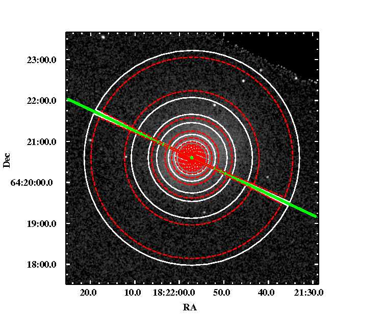
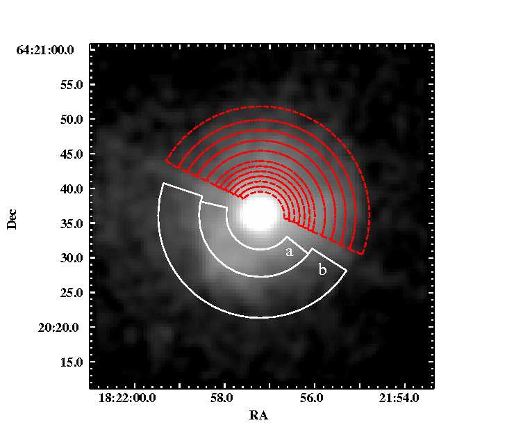
Figure 5: Exposure-corrected images in the 0.5–7.0$\rm\thinspace keV$ energy band smoothed with a 2D Gaussian $\sigma=1.5\arcsec$. Left: The regions for projected spectra are shown by the magenta dashed lines (referred to as 1-19 from the centre outwards) and those for deprojected spectra are shown by the white solid lines (referred to as a-i from the centre outwards). The readout streak, shown by the green box, and point sources were excluded. Right: Zoom in of central region showing the annuli affected by quasar emission (only half of each annulus is shown for clarity).

Figure 6: Spectrum and best-fitting model (solid line) for the inner dsdeproj deprojected spectra requiring a quasar emission model: deproj_a, $5-9\arcsec$ (upper), and deproj_b, $9-15\arcsec$ (lower). The model is a combination of a power-law model (dashed line) to account for the quasar emission and thermal plasma model (dotted line) for the cluster emission.

This analysis assumes that the detected X-rays from this source were produced either by the quasar nucleus or by bremsstrahlung and line emission from the ICM. However, there could be a contribution from X-ray synchrotron or inverse-Compton emission produced by the radio jets and lobes. The $1.7\rm\thinspace GHz$ MERLIN observation of H1821+643 showed that the radio jets were sited within a radius of $\sim 2\arcsec$, therefore an analysis of the X-ray emission at radii above $3\arcsec$ should not contain significant X-ray synchrotron radiation. The contribution of inverse-Compton emission, generated by relativistic plasma in the radio source lobes upscattering the jet-produced photons or the cosmic microwave background, was difficult to estimate. However, the spectra from $3\arcsec$ were well-described by the two component spectral fits incorporating the quasar and cluster emission and there is unlikely to be a significant extra contribution from inverse-Compton emission.

5 Results

5.1 Cluster surface brightness profile

The total surface brightness profile calculated from the exposure-corrected image for H1821+643 is shown in Fig. 7. The radial bins are 1″wide in the cluster centre and this was increased at larger radii where the background becomes more important. The simulated quasar PSF was subtracted from the total surface brightness profile to produce the cluster surface brightness profile. The flattening of the cluster profile from $15-20\arcsec$ corresponds to the surface brightness edge seen in Fig. 3. In addition, a second break in the cluster surface brightness profile can be seen at $\sim 8\arcsec$. The cluster surface brightness profile decreases in the innermost radial bin suggesting that the quasar component could have been overestimated.

Therefore, before proceeding with any analysis of these features, it was important to determine the uncertainty in the cluster surface brightness introduced by the quasar subtraction. This was achieved by comparing the observation and ChaRT simulation of 3C 273 as an estimate for the accuracy of the simulation of H1821+643. Fig. 7 shows a comparison of the ChaRT simulation of H1821+643 with the observation and simulation of 3C 273. The surface brightness profiles for 3C 273 were scaled by the ratio of the fluxes of the two quasars, determined from the respective readout streak spectra in the $0.5-7.0\rm\thinspace keV$ energy band. The ChaRT simulation was not expected to provide an exact prediction of the observed PSF, and indeed for 3C 273 the simulation underpredicts the observation, particularly in the PSF wings outside $10\arcsec$. The ChaRT model for the PSF wings is known to underestimate the wings and therefore this underestimation is likely to also be a problem for H1821+643.

However in H1821+643 the underprediction outside $10\arcsec$ is mitigated by the steep decline in the quasar contribution with radius compared to the cluster emission. For the region inside $10\arcsec$ where the subtraction is important, the simulation of 3C 273 underpredicts the observation by up to $\sim 10\%$. This offset could be due to the ChaRT model or alternatively caused by an underestimation in the modelling of the readout streak. Therefore, we estimated that the simulated quasar profile for H1821+643 could be offset by $\pm 10\%$ inside $10\arcsec$ radius. This offset did not significantly affect the quasar spectral parameters determined from the simulated spectra extracted in large radial bins, which were used to determine the cluster properties close to the nucleus (Fig. 19). However, for the cluster surface brightness profile, the offset resulted in an uncertainty of 25% in the innermost cluster profile radial bin, dropping to 5% by the third bin and then an insignificant contribution above $\sim 6\arcsec$ (Fig. 7). Therefore the decrease in cluster surface brightness observed in the central radial bin was not significant given the dominating contribution of the quasar.

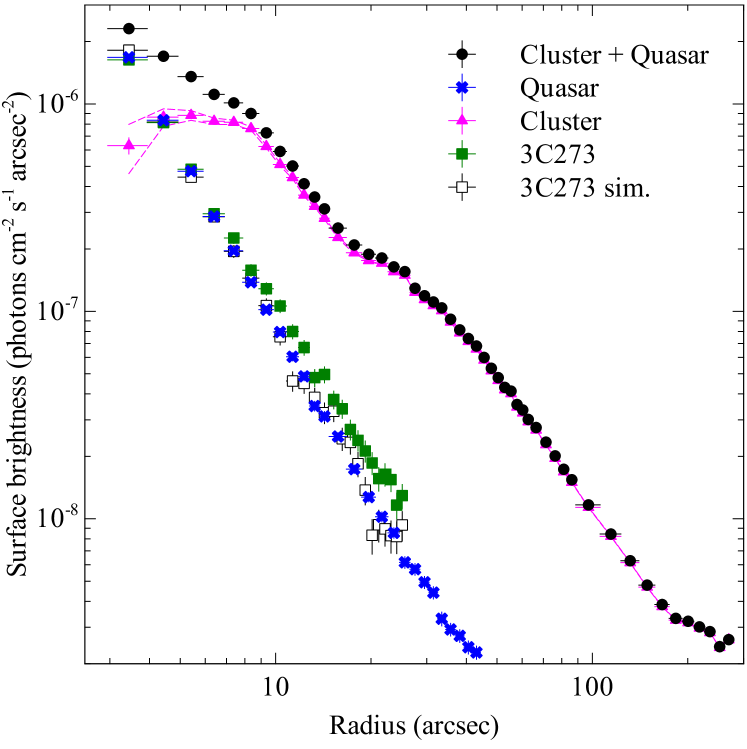
Figure 7: Total surface brightness profile in the energy range $0.5-7.0\rm\thinspace keV$ for H1821+643 (black circles), ChaRT simulation of the quasar surface brightness profile (blue crosses) and the cluster surface brightness profile produced by subtracting the quasar simulation from the total (magenta triangles). The surface brightness profile for 3C 273 (green squares) and corresponding simulation (white squares) are shown for comparison. The 3C 273 profiles have been normalized by the ratio of the $0.5-7.0\rm\thinspace keV$ fluxes as determined from the readout streaks. The magenta dashed lines show the effect of increasing and decreasing the quasar contribution by 10%.

The cluster surface brightness profile was also deprojected and evaluated in sectors (Fig. 8) to study the core structures. The width of the radial bins was increased from those of projected radial profile to ensure enough deprojected counts in each bin and produce a reliable deprojection. The quasar contribution was first subtracted from the total surface brightness profile. Then the resulting cluster surface brightness profile was deprojected by assuming spherical symmetry to subtract the contribution from the outer annuli off of the inner annuli. The region from $3-5\arcsec$ was excluded from the deprojection because the shallow gradient of the core surface brightness profile produced large errors in the values, in addition to the uncertainty from the quasar subtraction.

The SW sector (magenta) contains a section of the surface brightness edge at $\sim 15\arcsec$ but no extended emission from the core. Fig. 4 (right) suggests there could be a ‘ghost’ cavity from $5-12\arcsec$ in this sector. By analysing VLA $1.4\rm\thinspace GHz$ and MERLIN $1.7\rm\thinspace GHz$ observations, Blundell & Rawlings (2001) concluded that the jet axis in H1821+643 could be precessing. The ‘tipped over’ appearance of the N plume of radio emission in Fig. 3 is suggestive of this. The X-ray depressions to the NE and SW identified in Fig. 4 could have been inflated by the jet at an earlier time, detached and risen buoyantly as the jet precessed.

However the deprojected surface brightness profile does not appear to support this interpretation. Although there is less emission from this sector, the surface brightness profile inside $14\arcsec$ is smooth without the clear decrement expected from a cavity. It is therefore likely that the fractional difference image (Fig. 4 right) highlights the excess emission in the extended arms compared to the remaining emission at the same radius. However, cluster substructure and deviations from spherical symmetry in the cluster core will cause problems for the deprojection routine, particularly at radii inside the surface brightness edge. We cannot rule out the possibility that these features are ‘ghost’ cavities (X-ray cavities without any detected coincident radio emission).

The SE (green) and W (blue) sectors both contain extended arms of emission from the core and for the W sector this terminates particularly abruptly at the surface brightness edge at $15\arcsec$ (dashed line, Fig. 8 and Fig. 9). For these two sectors there is also evidence for an inner surface brightness edge at $8\arcsec$ (solid line, Fig. 8 and Fig. 9). Behind this inner edge, there could be a radio cavity in the SE sector. However, although the surface brightness profile is consistent with a decrease at this radius, there are only two radial bins in this region and they contain additional uncertainty associated with the quasar subtraction. Therefore, it is not clear whether this is a radio cavity.

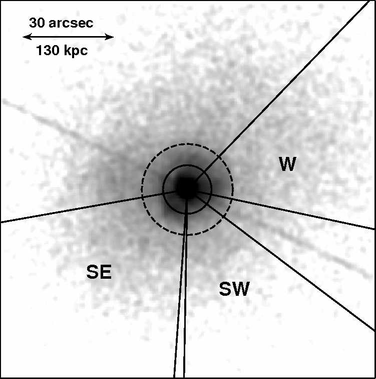
Figure 8: Exposure-corrected image in the 0.5–7.0$\rm\thinspace keV$ energy band smoothed with a 2D Gaussian $\sigma=1.5\arcsec$. The labelled sectors correspond to the area used to produce the surface brightness profiles in Fig. 9. The two surface brightness edges are marked with circles at $8\arcsec$ (solid) and $15\arcsec$ (dashed).

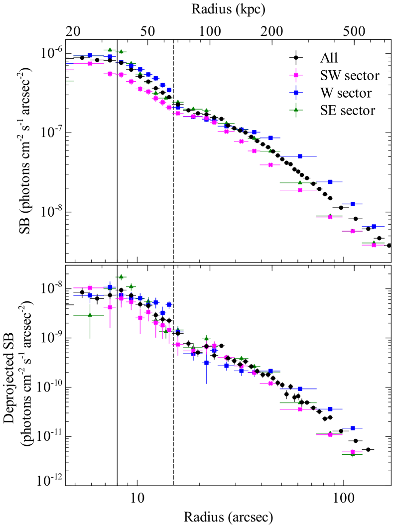
Figure 9: Top: quasar-subtracted surface brightness profiles in the energy range $0.5-7.0\rm\thinspace keV$ for H1821+643 extracted in sectors (Fig. 8) and the total surface brightness profile shown for comparison (black circles). Bottom: quasar-subtracted deprojected surface brightness profiles. The solid and dashed lines correspond to the circles in Fig. 8.

5.2 Projected Spectral Analysis

Fig. 10 shows the projected radial temperature and metallicity profiles for H1821+643 (also Table 2). The temperature profile shows a cool-core with a broad range in temperature, almost a factor of ten from the cluster outskirts down to $1.3\pm 0.2\rm\thinspace keV$ in the centre. The temperature starts to decline steeply at $\sim 18\arcsec$ and then breaks again at $\sim 7\arcsec$ for a sharp drop into the cluster centre. The metallicity is approximately constant at $\sim 0.3\hbox{$\thinspace\mathrm{Z}_{\odot}$}$ at large radii but increases in the cluster core to around $\sim 0.5\hbox{$\thinspace\mathrm{Z}_{\odot}$}$. The sudden drop in metallicity seen inside $6\arcsec$ is caused by an underestimate of the Fe K $\alpha$ line blend at $\sim 5\rm\thinspace keV$ (Figure 6). This is discussed in section 6.3.

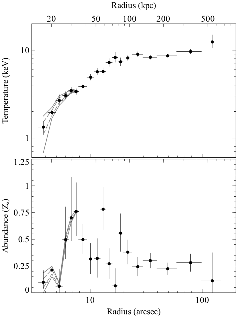
Figure 10: Projected radial temperature (upper) and metallicity (lower) profiles. The quasar contribution has been subtracted. The superimposed lines show the effect of varying the normalization of the quasar component by $\pm 10\%$ (dashed line) and $\pm 20\%$ (solid line).

We examined the systematic error in the projected radial profiles that could be introduced if the quasar normalization was varied by $\pm 10\%$ and $\pm 20\%$ and the power-law index varied by $\pm 0.05$. Fig. 10 shows that within a radius of $5\arcsec$ a variation of $\pm 20\%$ in normalization of the quasar component would add an uncertainty of $\pm 0.5\rm\thinspace keV$ to the cluster temperature value and $\pm 0.1\hbox{$\thinspace\mathrm{Z}_{\odot}$}$ to the metallicity. However, beyond $5\arcsec$ the contribution of the quasar PSF declines rapidly. Therefore this additional error is important only for the central two radial bins. Variation in the quasar power-law index did not produce significant additional error in the cluster parameters.

We applied spatially resolved spectroscopy techniques to produce maps of the projected temperature and pressure in the cluster core (Fig. 11). The central $\sim 4\times 4\arcmin$ was divided into bins using the Contour Binning algorithm (Sanders 2006), which follows surface brightness variations. Regions with a signal-to-noise ratio of 32 ($\sim 1000$ counts) were chosen, with the restriction that the length of the bins was at most two times their width. Background and quasar spectra from the ChaRT simulation were subtracted from the observed dataset and appropriate responses and ancillary responses were generated. Each spectrum was fitted with an absorbed mekal model with the absorption fixed to the Galactic value and the metallicity fixed to $0.4\hbox{$\thinspace\mathrm{Z}_{\odot}$}$. The spectra were grouped to contain a minimum of 20 counts per spectral channel and fitted in the energy range $0.5-7\rm\thinspace keV$. The fitting procedure minimised the $\chi^{2}$-statistic. The errors were approximately $\sim 10\%$ in temperature and $\sim 5\%$ for the emission measure.

Shown in Fig. 11 are the emission measure per unit area, temperature and ‘pressure’ maps. The ‘pressure’ map was produced by multiplying the emission measure per unit area and the temperature maps. The emission measure map shows the strongly peaked core surface brightness, which flattens in the very centre and the overall elongated morphology of the cluster in the NW to SE direction. The temperature in the cluster core drops down to $2\rm\thinspace keV$ and there is a region of cooler gas to the E forming part of a swirl, which could be similar to the spiral patterns seen in Abell 2029 (Clarke et al. 2004), Abell 2204 (Sanders et al. 2005) and in a temperature map of Perseus (Fabian et al. 2006).

The temperature map also shows an increase to the NW from $15-20\arcsec$ coincident with the strongest section of the surface brightness edge (Fig. 9). This temperature increase is also found in a projected temperature profile extracted in the NW sector (Fig. 8), however this increase is not statistically significant enough to draw any further conclusions on the nature of the surface brightness edge. In addition, the pressure map does not show a particularly sharp drop from $15-20\arcsec$ which would indicate a shock.

It is not obvious from any of the maps shown in Fig. 11 in which direction the main radio axis is oriented. Apart from a small low pressure region to the SE, which could relate to the small radio bubble, the pressure map appears symmetric about the central source with no indication that it contains a large FR I source.

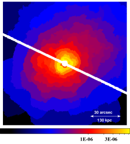
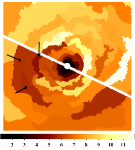
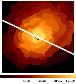
Figure 11: Left: emission measure per unit area map (units $\hbox{$\rm\thinspace cm^{-5}\,$}\rm\thinspace arcsec^{-2}\,$). The emission measure is the xspec normalization of the mekal spectrum $K=EI/(4\times 10^{14}\pi D_{A}^{2}(1+z)^{2})$, where EI is the emission integral $EI=\int n_{e}n_{H}\mathrm{d}V$. Centre: temperature map ($\rm\thinspace keV$) with arrows marking the possible swirl of cool gas. Right: ‘pressure’ map ($\rm\thinspace keV\hbox{$\rm\thinspace cm^{-5}\,$}\rm\thinspace arcsec^{-2}\,$) produced by multiplying the emission measure and temperature maps. The maps cover the same spatial scale and the quasar contribution has been subtracted. The readout streak and central $3\arcsec$ radius region affected by pileup have been masked out.

Table 2: Table of best-fitting cluster parameters for each projected region. Column 1) Region name 2) Inner and outer radii of annulus (″) 3) Temperature ($\rm\thinspace keV$) 4) Abundance ($\thinspace\mathrm{Z}_{\odot}$) 5) $\chi^{2}$ / number of degrees of freedom

Region	Radius	Temp.	Abund.	$\chi^{2}$/dof
proj1	3.4–4.2	$1.3\pm 0.2$	$0.10^{+0.11}_{-0.06}$	15/24
proj2	4.2–4.9	$2.0^{+0.3}_{-0.2}$	$0.2^{+0.2}_{-0.1}$	26/25
proj3	4.9–5.7	$2.7^{+0.4}_{-0.3}$	$0.06^{+0.16}_{-0.06}$	26/25
proj4	5.7–6.4	$3.0\pm 0.3$	$0.5^{+0.3}_{-0.2}$	26/27
proj5	6.4–7.1	$3.5\pm 0.3$	$0.7^{0.4}_{-0.2}$	29/26
proj6	7.1–7.9	$3.4^{+0.3}_{-0.2}$	$0.8^{+0.3}_{-0.2}$	27/27
proj7	7.9–9.3	$3.9\pm 0.2$	$0.5\pm 0.1$	38/51
proj8	9.3–10.8	$4.9^{+0.4}_{-0.3}$	$0.3\pm 0.1$	57/50
proj9	10.8–12.3	$5.7^{+0.6}_{-0.5}$	$0.3\pm 0.2$	22/41
proj10	12.3–13.8	$5.7^{+0.6}_{-0.5}$	$0.8\pm 0.2$	34/36
proj11	13.8–15.7	$7.2^{+0.8}_{-0.7}$	$0.3\pm 0.1$	44/44
proj12	15.7–17.7	$8\pm 1$	$0.06^{+0.16}_{-0.06}$	42/40
proj13	17.7–19.7	$7.4^{+0.8}_{-0.7}$	$0.6\pm 0.2$	38/39
proj14	19.7–23.6	$8.2^{+0.7}_{-0.6}$	$0.4\pm 0.1$	90/75
proj15	23.6–29.5	$9.0\pm 0.6$	$0.24\pm 0.09$	119/110
proj16	29.5–39.4	$8.3\pm 0.4$	$0.30\pm 0.07$	166/150
proj17	39.4–59.0	$8.6\pm 0.4$	$0.22\pm 0.06$	206/183
proj18	59.0–98.4	$9.7^{+0.6}_{-0.5}$	$0.28\pm 0.08$	236/214
proj19	98.4–147.6	$12^{+3}_{-2}$	$0.1^{+0.3}_{-0.1}$	195/209

Table 3: Table of best-fitting cluster parameters for each deprojected region. Column 1) Region name 2) Inner and outer radii of annulus (″) 3) Temperature ($\rm\thinspace keV$) 4) Electron density ($\rm\thinspace cm^{-3}\,$) 5) Abundance ($\thinspace\mathrm{Z}_{\odot}$) 6) $\chi^{2}$ / number of degrees of freedom

Region	Radius	Temp.	$n_{e}$	Abund.	$\chi^{2}$/dof
			($\times 10^{-3}$)
deproja	4.9–8.9	$2.4\pm 0.2$	$46\pm 2$	$0.4^{+0.2}_{-0.1}$	72/58
deprojb	8.9–14.8	$4.3^{+0.4}_{-0.3}$	$26.0^{+0.6}_{-0.5}$	$0.2\pm 0.1$	71/58
deprojc	14.8–24.6	$7.7^{+1.0}_{-0.8}$	$11.7\pm 0.3$	$0.5\pm 0.2$	64/58
deprojd	24.6–34.4	$7.7^{+1.0}_{-0.8}$	$8.8\pm 0.2$	$0.5\pm 0.2$	66/58
deproje	34.4–51.7	$7.6^{+0.8}_{-0.6}$	$5.41\pm 0.09$	$0.4\pm 0.2$	69/58
deprojf	51.7–64.0	$10^{+3}_{-1}$	$3.8\pm 0.1$	$0.2^{+0.3}_{-0.2}$	51/58
deprojg	64.0–88.6	$8.5^{+1.0}_{-0.8}$	$2.50\pm 0.05$	$0.3\pm 0.2$	46/58
deprojh	88.6–157.4	$12^{+2}_{-2}$	$1.08^{+0.02}_{-0.03}$	$0.1^{+0.3}_{-0.1}$	45/58

5.3 Deprojected Radial Profiles

Fig. 12 shows the deprojected radial profiles for both the surface brightness and spectral deprojection methods applied to H1821+643. The results for the spectral deprojection are also listed in Table 3. The surface brightness deprojection produced a mass profile with a concentration $c=1.3^{+0.9}_{-0.7}$ and $r_{200}=2.5^{+1.3}_{-0.7}\rm\thinspace Mpc$. The spatial region from $3-5\arcsec$ was excluded from the deprojection analysis because the shallow gradient of the core surface brightness profile and the core cluster substructure produced large errors in the parameters, in addition to the uncertainty from the quasar subtraction (Fig. 7).

The deprojected temperature profile shows a steep drop inside the central $100\rm\thinspace kpc$, from $10^{+1}_{-3}\rm\thinspace keV$ at $\sim 250\rm\thinspace kpc$ down to $2.5^{+0.2}_{-0.2}\rm\thinspace keV$ in the cluster centre. The surface brightness deprojection result is similar but shows an increase in temperature within the central $40\rm\thinspace kpc$. This appears to correlate with a decrease in the electron density, calculated from the emission measure of the deprojected spectrum, however the errors are consistent with a flat profile. Although there is a break in the density profile at $\sim 15\arcsec$ corresponding to the surface brightness edge, there does not appear to be a sharp discontinuity to indicate a shock. A jump in either temperature or density cannot be discerned for the dsdeproj result because large radial bins were required to ensure enough counts for a good deprojection. The assumption of hydrostatic equilibrium in the surface brightness deprojection would also have smeared out any discontinuity associated with a shock. Finally, the surface brightness edge is not radially symmetric about the quasar. Therefore the circular annuli centred on the quasar that were used for the deprojection will have inevitably smeared the spectrum from this region over neighbouring annuli. Deprojecting the cluster in the NW sector (Fig. 8) where the edge is strongest and narrowest would be more likely to produce a conclusion about its nature, however there are not enough X-ray counts to deproject in sectors. It was therefore not possible to determine unequivocally the nature of the surface brightness edge with the available data.

The metallicity profile produced by spectral deprojection is consistent with a constant value of $\sim 0.4\hbox{$\thinspace\mathrm{Z}_{\odot}$}$ in the core, decreasing to $0.2-0.3\hbox{$\thinspace\mathrm{Z}_{\odot}$}$ at large radii. The assumption of a constant abundance of $0.4\hbox{$\thinspace\mathrm{Z}_{\odot}$}$ for the surface brightness deprojection was therefore deemed to be suitable.

Both deprojections were repeated with a $\pm 10\%$ variation in the subtracted quasar contribution. This resulted in an uncertainty of $\pm 0.1\rm\thinspace keV$ for the innermost annuli in the surface brightness deprojection, smaller than the statistical error of $\pm 0.3\rm\thinspace keV$. The variation produced a $\pm 0.2\rm\thinspace keV$ uncertainty for the innermost bin of the dsdeproj result but was insignificant at larger radii. The increase in the central temperature shown in the surface brightness deprojection is therefore an inconsistency between the two deprojection methods. A finer spatial binning over the inner radii was tried for the spectral deprojection in order to confirm this feature. However, the flat surface brightness profile in the core resulted in a larger fraction of projected emission in each annulus. Therefore, increasing the number of annuli to be deprojected produced much larger uncertainties in the central shell. The increase in core temperature is not seen in the projected temperature profile (Fig. 10) or the temperature map (Fig. 11). Whilst the lack of confirmation in projected profiles or the alternative, low resolution deprojection method does not preclude an increase in core temperature, the feature could instead be an artifact of the deprojection method.

The additional assumptions of hydrostatic equilbrium and an NFW mass model made by the surface brightness deprojection method might not be appropriate for the cluster core. For a sample of fourteen galaxy clusters observed with Chandra, Voigt & Fabian (2006) found that the mass distribution for the majority of the objects was consistent with the NFW model, however four objects in the sample exhibited a flatter core. Forcing an NFW mass model in the cluster core when the gas mass was in fact much lower could, via hydrostatic equilibrium, artificially boost the calculated ICM temperature. Structural features in the cluster core, such as a shock or dense blob of gas, are also expected to cause spurious deprojection results.

By combining the deprojected temperature $T$ and electron density $n_{e}$, we calculated derived properties such as the electron pressure $P_{e}=k_{B}n_{e}T$, radiative gas cooling time

$$t_{\mathrm{cool}}=\frac{5}{2}\frac{nk_{B}T}{n_{e}n_{H}\Lambda(T)}$$ (1)

where $\Lambda(T)$ is the cooling function, and entropy $S=k_{B}Tn_{e}^{-2/3}$. We assumed the temperature and density were independent of each other in order to calculate errors on the derived quantities. The majority of the error was in the temperature values so this was a reasonable assumption.

Fig. 13 shows the electron pressure increases steadily towards the cluster core. However, beyond the surface brightness edge the dsdeproj result flattens possibly to a constant pressure within $50\rm\thinspace kpc$. The surface brightness deprojection result assumes hydrostatic equilibrium and an NFW mass model, which constrain the pressure profile. Therefore this conflicting result may indicate that the radio source provides a significant source of non-thermal pressure in the cluster core. The value of the pressure for the innermost radial bin in the spectral deprojection result should be considered a lower limit on the total pressure. It is therefore difficult to determine whether there is a jump in pressure across the surface brightness edge at $13-17\arcsec$ indicating a shock. If instead the pressure smoothly changes across this region the feature could be a cold front (see Markevitch & Vikhlinin 2007 and references therein).

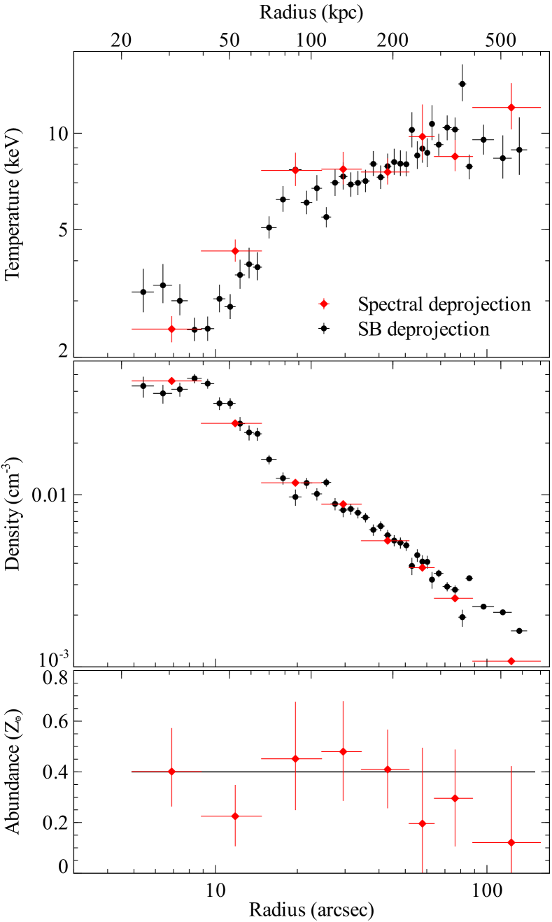
Figure 12: Quasar-subtracted deprojected temperature (top), electron density (centre) and metallicity (bottom) profiles for the spectral deprojection method (red diamonds) and the surface brightness deprojection method (black circles). The radius extends in to 3″to enable a comparison with Fig. 10.

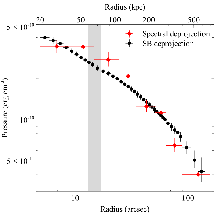
Figure 13: Quasar-subtracted deprojected electron pressure profile for the spectral deprojection method (red diamonds) and the surface brightness deprojection method (black circles). The shaded region denotes the radial extent of the surface brightness edge from $13-17\arcsec$.

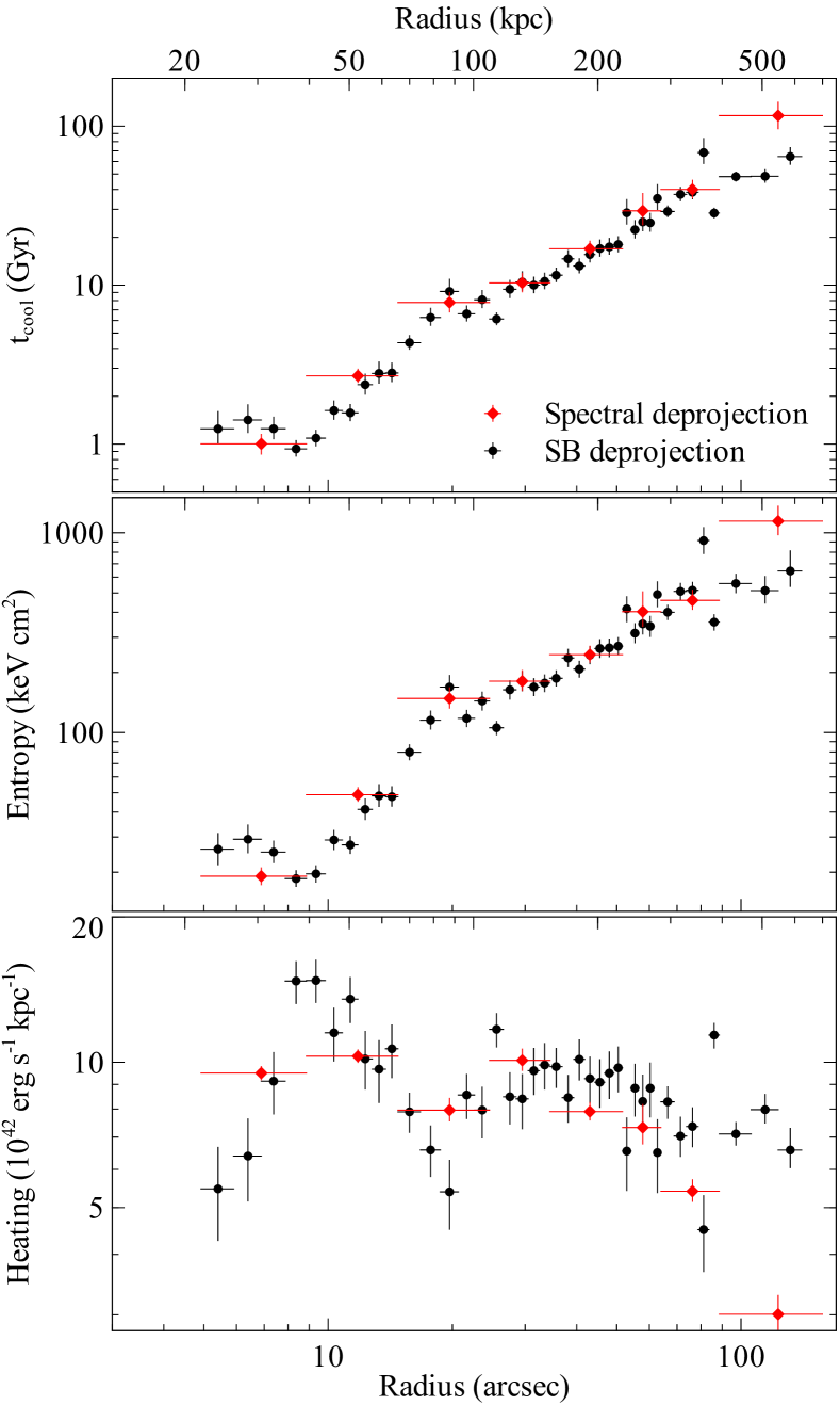
Figure 14: Quasar-subtracted deprojected ICM cooling time (top), entropy (centre) and heating rate required per $\rm\thinspace kpc$ width shell (bottom) profiles for the spectral deprojection method (red diamonds) and the surface brightness deprojection method (black circles). The radius extends in to 3″to enable a comparison with Fig. 10.

The gas cooling time falls steadily down to $1.0^{+0.1}_{-0.1}\rm\thinspace Gyr$ at a radius of 7″($30\rm\thinspace kpc$) in the core of the cluster (Fig. 14). With such a short central gas cooling time, we would expect that gas might be cooling down below X-ray temperatures. The cooling radius was defined to be the radius at which the cooling time fell to $7.7\rm\thinspace Gyr$, the time since $z=1$. The cooling radius of H1821+643 is at 20″($90\rm\thinspace kpc$). The X-ray mass deposition rate inside the cooling radius was calculated by using the xspec mkcflow model, which models the emission from gas cooling between two temperatures where the normalization is the mass of cooling gas.

The dsdeproj deprojection process was therefore repeated using a larger innermost annulus $5-20\arcsec$ ($22-90\rm\thinspace kpc$). However, the majority of the mass deposition in clusters occurs in the cluster centre, where the radiative gas cooling times are shortest. The crucial inner $20\rm\thinspace kpc$ was necessarily excluded from our analysis, therefore to get an upper limit on the mass deposition rate, we assumed a single-phase cooling flow and fitted a phabs(pow)+phabs(mekal+mkcflow) model to the cooling region spectrum in xspec. The lower temperature of the mkcflow component was therefore fixed to $1\rm\thinspace keV$ and the higher temperature was tied to the temperature parameter in the mekal component. The abundance was fixed to $0.4\hbox{$\thinspace\mathrm{Z}_{\odot}$}$. The quasar spectral properties were calculated as before by fitting to the ChaRT simulation of the cluster spectrum from the cooling region. The spectral fit resulted in an upper limit on the mass deposition rate of $300\pm 100\hbox{$\hbox{$\rm\thinspace M_{\odot}$}\rm\thinspace yr^{-1}\,$}$ within the cooling radius. Direct detections of the amount of gas cooling out of the X-ray requires deep high resolution spectroscopy (eg. Peterson et al. 2003).

The heating rate refers to the spatial distribution in heat required to balance the cooling of the cluster gas and was calculated by dividing the total X-ray luminosity in each shell by the shell width. Fig. 14 shows that the rate at which energy must be deposited in shells of equal width is approximately constant at $10^{43}\hbox{$\rm\thinspace erg\rm\thinspace s^{-1}\rm\thinspace kpc^{-1}\,$}$ within $100\rm\thinspace kpc$, decreases in the radial bin associated with the surface brightness edge, and then drops off beyond $200\rm\thinspace kpc$. The total required heating rate to balance the cooling losses within the cooling radius is therefore $\sim 10^{45}\hbox{$\rm\thinspace erg\rm\thinspace s^{-1}\,$}$.

5.4 Potential cavity heating

Assuming the X-ray depression at a distance of $24\rm\thinspace kpc$ from the nucleus is a radio cavity (Fig. 4), we follow the method of Dunn & Fabian (2004) (see also Bîrzan et al. 2004) to calculate the cavity heating power. The energy input of the cavity is the sum of the cavity’s internal energy and the work done,

$$E=\frac{1}{\gamma-1}PV+P\mathrm{d}V\approx\frac{\gamma}{\gamma-1}PV,$$ (2)

where $P$ is the thermal pressure of the surrounding ICM, $V$ is the volume of the cavity and $\gamma$ is the mean adiabatic index of the fluid in the cavity. The relativistic case of $\gamma=4/3$ was assumed.

We used two different methods to place upper and lower limits on the potential cavity heating power. For a lower limit, we assumed there is no additional non-thermal pressure in the cluster core and used the dsdeproj weak pressure gradient shown in Fig. 13. For an upper limit, the gas pressure profile from $40-150\rm\thinspace kpc$ was extrapolated inwards using a powerlaw to produce an estimate of the total central pressure, similar to the surface brightness deprojection result. The instantaneous mechanical power for the cavity is $P_{\mathrm{bubble}}=4PV/t_{\mathrm{age}}$, where $t_{\mathrm{age}}$ is the bubble age. The cavity was assumed to be spherical with a radius of $\sim 9\rm\thinspace kpc$, estimated from the image using a circular aperture, and located at a distance of $\sim 24\rm\thinspace kpc$ from the cluster centre. Two estimates of the cavity age are commonly used: the time required for the cavity to rise to its current location at the speed of sound, $t_{\mathrm{sound}}$, and the time required for the cavity to rise buoyantly at its terminal velocity, $t_{\mathrm{buoy}}$. The sound speed timescale is more applicable to young radio cavities recently inflated by the AGN. Its value was $0.03\rm\thinspace Gyr$, which gives a cavity heating power of $1-2\times 10^{44}\hbox{$\rm\thinspace erg\rm\thinspace s^{-1}\,$}$.

Although there could be extra AGN heating power produced by weak shocks and sound waves (Fabian et al. 2006), cavity heating in H1821+643 is not currently supplying enough heat to replace the majority of the $\sim 10^{45}\hbox{$\rm\thinspace erg\rm\thinspace s^{-1}\,$}$ radiated by the cluster gas. The possible ‘ghost’ cavities could potentially produce an additional power of $9\times 10^{44}\hbox{$\rm\thinspace erg\rm\thinspace s^{-1}\,$}$, calculated using the buoyancy timescale. However, it is not clear from the deprojected surface brightness profiles (Fig. 9) that these features are cavities.

6 Discussion

6.1 Evidence for quasar and cluster interactions

The morphology in the central $100\rm\thinspace kpc$ of H1821+643 suggests a complex interaction between the quasar and the surrounding cluster gas. There are extended arms of emission and an inner radio cavity with a bright rim in the core and a weak shock or cold front surrounding most of the cluster core at $\sim 15\arcsec$. However, the mechanisms by which the quasar output is coupled to the ICM are far from clear.

The extended arms of X-ray emission to the N and SE appear to be correlated with the main axis of the extended FR I radio emission. These X-ray features may have been pushed or dragged out from the cluster core by the expanding FR I structure. Although the inner radio cavity is too close to the quasar to be analysed effectively, this indicates that there could be some mechanical feedback in the cluster core. The ends of the FR I structure appear to terminate at the surface brightness edge seen in the X-ray so this feature could be a weak shock generated by the radio source expanding into surrounding cluster gas. However, Blundell & Rawlings (2001) found that the outermost ends of the extended radio emission do not appear to end in shocks. They inferred that the extended emission has not grown any faster than the ambient sound speed of the ICM. In addition, the extended X-ray structure to the W is not associated with any radio emission and the surface brightness edge appears strongest in this radial direction (Fig. 9).

Based on optical imaging, Hutchings & Neff (1991) suggested that H1821+643 is in the late stages of a mild tidal event or merger, although there is no sign of a disturbing object. Fried (1998) found that the line widths of the extended emission-line gas in H1821+643 produced velocity dispersions in agreement with this interaction scenario. However, velocity dispersions of a few hundred $\rm\thinspace km\rm\thinspace s^{-1}\,$ are also consistent with the kinematics of emission-line nebulae in cool-core clusters (Hatch et al. 2007). The X-ray features could be interpreted as resulting from a merger interaction which has disturbed the gas in the cluster core. Blundell & Rawlings (2001) estimated that if the radio plumes have emerged no faster than the ambient sound speed then the radio structure has been stable for a minimum of $3\times 10^{8}\rm\thinspace yr$. The surface brightness edge could be a weak shock generated by a merger at that time or more likely, given that it can be observed around most of the cluster core, it could be a cold front produced by the cool-core gas sloshing in the cluster potential well (Markevitch et al. 2000; Vikhlinin et al. 2001). The swirl feature seen in the projected temperature map would also support this interpretation (Fig. 11).

H1821+643 shows no obvious evidence for X-ray absorbing winds from the quasar in the Chandra HETG (Fang et al. 2002), LETG (Mathur et al. 2003) or in FUSE spectra (Oegerle et al. 2000). However, outflows could be oriented in the plane of the sky and therefore not evident along our line of sight. Oegerle et al. (2000) observed associated absorption at the redshift of H1821+643 in the FUSE and HST spectra (see also Bahcall et al. 1992) and concluded that this was unlikely to be quasar intrinsic absorption. Instead they proposed that the broad range of ionization present required a multiphase absorber that is likely located in the central cluster galaxy. We found that the X-ray spectra for the central two annuli, that cover the spatial extent of the central galaxy, did not require any additional absorption above the Galactic column density determined by Kalberla et al. (2005). However, these annuli contain a significant fraction of the quasar PSF and any additional absorption contribution to the spectrum was difficult to determine. We compared soft ($0.5-1.0\rm\thinspace keV$ and $1.0-2.0\rm\thinspace keV$) and hard band ($3.0-7.0\rm\thinspace keV$) images to see if there were any obvious potential sites for absorption. The X-ray depression at $24\rm\thinspace kpc$ from the nucleus was clearly visible in both soft band images, surrounded by cool rims of gas, however it was not visible in the hard band image. The hard band image contains far fewer counts and was dominated by the quasar PSF. Therefore a small cavity would be particularly difficult to distinguish. However, this could also be interpreted as a cool extended arm of emission, similar to those in the N and NW directions, with a superimposed absorption region.

6.2 Accretion Mechanisms

The total energy output, radiative and mechanical, of the AGN can be used to infer an accretion rate for H1821+643, assuming an accretion efficiency for each mechanism. Using a bolometric correction of 50 from Vasudevan & Fabian (2007) with the quasar luminosity in the energy range $2-10\rm\thinspace keV$ $L_{X}=(4.2\pm 0.1)\times 10^{45}\hbox{$\rm\thinspace erg\rm\thinspace s^{-1}\,$}$, we calculated the quasar bolometric luminosity $L_{\mathrm{bol}}\sim 2\times 10^{47}\hbox{$\rm\thinspace erg\rm\thinspace s^{-1}\,$}$. However, this could have been underestimated if a significant number of X-ray photons from the quasar were scattered by the ICM. By extrapolating the electron density profile in to $\sim 0.1\hbox{$\rm\thinspace cm^{-3}\,$}$, we estimated an optical depth for the central $30\rm\thinspace kpc$ region of $\tau\sim 0.002$. Therefore, only $\sim 1$ in 1000 photons from the quasar would be scattered by the ICM and this effect is insignificant.

For a radiative efficiency $\epsilon=0.1$, the mass accretion rate required to power the quasar is therefore $\dot{M}_{\mathrm{acc}}=L_{\mathrm{bol}}/\epsilon c^{2}\sim 40\hbox{$\hbox{$\rm\thinspace M_{\odot}$}\rm\thinspace yr^{-1}\,$}$. The mechanical power calculated by cavity heating is several orders of magnitude lower than the quasar luminosity and therefore is not included in an estimate of the required accretion rate. The calculated mass accretion rate for H1821+643 can be compared with the theoretical Eddington and Bondi accretion rates.

The Eddington accretion rate can be expressed as

$$\frac{\dot{M}_{\mathrm{Edd}}}{\hbox{$\hbox{$\rm\thinspace M_{\odot}$}\rm\thinspace yr^{-1}\,$}}=\frac{6.6}{\epsilon}\left(\frac{M_{BH}}{3\times 10^{9}\hbox{$\rm\thinspace M_{\odot}$}}\right)$$ (3)

Using the H$\alpha$, H$\beta$ and MgII line widths and the optical/UV continuum luminosity (Kolman et al. 1993), together with the recipes in McGill et al. (2008) (their section 4.1 and references therein) we estimated a black hole mass $M_{BH}\sim 3\times 10^{9}\hbox{$\rm\thinspace M_{\odot}$}$ for H1821+643. The uncertainties in the bolometric correction and the black hole mass were at least 50% and therefore subsequent calculations were assumed to be only an estimate. Using the estimate of black hole mass, the Eddington luminosity was calculated to be $L_{\mathrm{Edd}}\sim 4\times 10^{47}\hbox{$\rm\thinspace erg\rm\thinspace s^{-1}\,$}$, giving an Eddington accretion rate $\dot{M}_{\mathrm{Edd}}\sim 70\hbox{$\hbox{$\rm\thinspace M_{\odot}$}\rm\thinspace yr^{-1}\,$}$ and a high Eddington ratio $L_{\mathrm{bol}}/L_{\mathrm{Edd}}\sim 0.5$.

Assuming spherical symmetry and negligible angular momentum, the Bondi rate is the rate of accretion for a black hole with an accreting atmosphere of temperature, $T$, and density, $n_{e}$, (Bondi 1952) and can be expressed as

$$\frac{\dot{M}_{\mathrm{Bondi}}}{\hbox{$\hbox{$\rm\thinspace M_{\odot}$}\rm\thinspace yr^{-1}\,$}}=0.12\left(\frac{k_{B}T}{\rm\thinspace keV}\right)^{-3/2}\left(\frac{n_{e}}{\hbox{$\rm\thinspace cm^{-3}\,$}}\right)\left(\frac{M_{BH}}{3\times 10^{9}\hbox{$\rm\thinspace M_{\odot}$}}\right)^{2}$$ (4)

for an adiabatic index $\gamma=5/3$. This accretion occurs within the Bondi radius, $r_{\mathrm{Bondi}}$, within which the gravitational potential of the black hole dominates over the thermal energy of the surrounding gas,

$$\frac{r_{\mathrm{Bondi}}}{\rm\thinspace kpc}=0.10\left(\frac{k_{B}T}{\rm\thinspace keV}\right)^{-1}\left(\frac{M_{BH}}{3\times 10^{9}\hbox{$\rm\thinspace M_{\odot}$}}\right).$$ (5)

The Bondi accretion rate is therefore an estimate of the rate of accretion from the hot ICM directly onto the black hole. The Bondi radius is not resolved for H1821+643 so the electron density and temperature from the innermost annulus were used as lower and upper limits, respectively, on the accretion atmosphere properties producing an underestimate of the Bondi accretion rate. For an innermost temperature $2.4\pm 0.2\rm\thinspace keV$ and electron density $0.046\pm 0.002\hbox{$\rm\thinspace cm^{-3}\,$}$, the Bondi accretion rate is estimated to be $\dot{M}_{\mathrm{Bondi}}\sim 0.001\hbox{$\hbox{$\rm\thinspace M_{\odot}$}\rm\thinspace yr^{-1}\,$}$ at the Bondi radius $r_{\mathrm{Bondi}}\sim 40\rm\thinspace pc$. Although this estimate of the Bondi accretion rate is expected to lie below the true value, the implied accretion rate for the quasar exceeds this by a factor of $\sim 10^{4}$.

Following Allen et al. (2006), we also estimated the Bondi accretion rate by extrapolating the temperature and density of the cluster gas in to the Bondi radius. This was achieved by using powerlaw fits to the inner annuli of the dsdeproj deprojected temperature and density profiles in Fig. 12. The steep temperature ($T(r)\propto r^{0.6}$) and density gradients ($n_{e}(r)\propto r^{-1.2}$) in the cool-core produced an upper limit on the Bondi accretion rate of $\dot{M}_{\mathrm{Bondi}}\sim 6\hbox{$\hbox{$\rm\thinspace M_{\odot}$}\rm\thinspace yr^{-1}\,$}$ at $r_{\mathrm{Bondi}}\sim 0.5\rm\thinspace kpc$. However, an extrapolation over two orders of magnitude in radius is unlikely to provide a good estimate of the Bondi accretion rate. Allen et al. (2006) analysed elliptical galaxies, which had shallow central temperature gradients and X-ray data permitting a measurement of the gas properties within one order of magnitude of the Bondi radius.

Compton cooling of the accretion flow by radiation from the quasar could potentially increase the flow of material from a hot atmosphere onto the black hole (Fabian & Crawford 1990). Since Compton scattering between strong UV photons and hot electrons can dominate the cooling process for the ICM in the cluster core, accretion by Compton cooling can supply gas to the central black hole and, as shown by Fabian & Crawford (1990), the accretion rate by Compton cooling flow can be larger than that of Bondi accretion alone. Using the cluster gas properties in the innermost annulus, we determined that Compton cooling will dominate bremsstrahlung cooling within a radius $R_{C}\sim 5\rm\thinspace kpc$ and rapidly cool the gas down to the Compton temperature.

The Compton temperature was calculated using the quasar spectral energy distribution (SED) from the optical to the soft X-ray presented in Kolman et al. (1993). We fitted the SED in xspec with their Kerr disk model for the UV bump (Fig. 16(c) in Kolman et al. 1993) and a broken power-law to provide an extension up to $100\rm\thinspace keV$, as described in Vasudevan & Fabian (2009). Therefore, with the bulk of the emitted quasar luminosity in the UV, the Compton temperature is $T_{C}\sim 0.4\rm\thinspace keV$.

If the accreting material is quickly Compton cooled within $\sim 5\rm\thinspace kpc$, as it approaches the Bondi radius, then the Bondi radius will grow from $r_{\mathrm{Bondi}}\sim 40\rm\thinspace pc$ to $\sim 250\rm\thinspace pc$ and the Bondi accretion rate increases from $\dot{M}_{\mathrm{Bondi}}\sim 0.001\hbox{$\hbox{$\rm\thinspace M_{\odot}$}\rm\thinspace yr^{-1}\,$}$ to $\sim 6\hbox{$\hbox{$\rm\thinspace M_{\odot}$}\rm\thinspace yr^{-1}\,$}$. Therefore, Bondi accretion of rapidly Compton cooled material could provide a significant source of fuel for the quasar.

Cold accretion mechanisms, such as the cold feedback scenario suggested by Pizzolato & Soker (2005), could provide an alternative route for accreting material. Within the cooling region of H1821+643, up to $300\pm 100\hbox{$\hbox{$\rm\thinspace M_{\odot}$}\rm\thinspace yr^{-1}\,$}$ could be cooling down below X-ray temperatures. Pizzolato & Soker (2005) proposed that overdense blobs of cool gas from within the entire cooling region rapidly cool and sink towards the central black hole or condense to form cold molecular clouds and stars. A large influx of material onto the black hole, caused by an accretion disk instability for example, would then trigger an outburst. For cold accretion to provide a source of fuel for the quasar, a significant fraction of the gas cooling out of the X-ray must be funnelled down onto the black hole. Such an efficient, steady accretion of material from within the cooling region seems unlikely, however the cooling material could have built up in the cluster centre to form a large reservoir of cool gas which feeds the nucleus after a triggering event.

Alternatively, a merger scenario could have initiated the quasar outburst by providing a rapid influx of fuel for the central engine. The precession in the jet axes suggested by the observations of Blundell & Rawlings (2001) could have arisen if the central engine was composed of two orbiting black holes that had not yet merged. A merger scenario could therefore potentially have triggered the quasar outburst and the jet precession. However, the galaxy cluster’s deep gravitational potential will tidally strip a merging subcluster of its gas in the cluster outskirts, making it difficult to channel the merging material effectively down onto the central black hole.

6.3 Impact of the quasar on the galaxy cluster core

Fig. 15 compares the radiative gas cooling time profiles of H1821+643 with a sample of 16 cool-core and non-cool-core clusters with Chandra archival observations. The clusters were roughly selected on redshift ($z=0.06-0.25$) and the number of X-ray counts in the Chandra observation. The first criterion ensured a similar intrinsic spatial extent on the ACIS chip to H1821+643 and the second provided an equivalent resolution with at least eight deprojected radial bins ($\sim 40,000$ counts). In addition, three non-cool-core clusters, Abell 1650, Abell 2142 and Abell 2244, were included to serve as a contrast.

H1821+643 has a cooling time profile typical of a strong cool-core cluster with a more passive central engine, such as Abell 1835. Underneath the quasar, the large-scale properties of the galaxy cluster have not been strongly affected and the ICM is continuing to evolve in a similar way to other cool-core clusters.

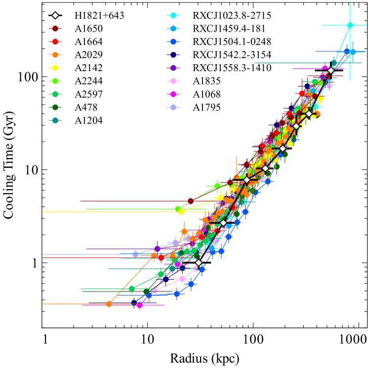
Figure 15: dsdeproj deprojected gas cooling times for a sample of cool-core and non-cool-core galaxy clusters.

This period of quasar activity in H1821+643 is unlikely to be long-lived. For such a high accretion rate of $40\hbox{$\hbox{$\rm\thinspace M_{\odot}$}\rm\thinspace yr^{-1}\,$}$, the e-folding time of the SMBH growth, assuming a radiative efficiency $\epsilon=0.1$, is $\sim 10^{8}\rm\thinspace yr$ and in this time the SMBH would need to accrete $\sim 4\times 10^{9}\hbox{$\rm\thinspace M_{\odot}$}$ of material. A period of rapid black hole growth longer than $\sim 10^{8}\rm\thinspace yr$ would therefore result in a black hole mass far larger than the typical upper limit observed (eg. Marconi et al. 2004 and references therein). On this timescale, we would not expect radiative heating from the quasar to significantly alter the gas cooling time calculated in large radial bins. However, to quantify the effect of the active nucleus on the cluster gas we have run Cloudy (version 08.00) (Ferland et al. 1998) models appropriate to conditions in the regions $15-30\rm\thinspace kpc$ (projected) and $22-39\rm\thinspace kpc$ (dsdeproj deprojected) from the nucleus.

The Cloudy simulations are described in detail in Appendix B. In summary, we generated the intrinsic continuum shape for the active nucleus using the quasar SED model described in section 6.2. A model of the cluster gas, with suitable temperature $2.4\rm\thinspace keV$ and metallicity $0.4\hbox{$\thinspace\mathrm{Z}_{\odot}$}$, at the distance of the extracted X-ray spectrum was then irradiated with this quasar continuum. The emitted spectrum of the Cloudy model, together with a model accounting for the quasar PSF, were fitted to the observed spectra from the projected ($15-30\rm\thinspace kpc$) and deprojected ($22-39\rm\thinspace kpc$) regions. We also produced a Cloudy model for only the cluster emission to provide a simple comparison for the Cloudy model with the added quasar contribution.

The addition of the Cloudy quasar component did not significantly alter the shape of the model spectrum (Fig. 16). However in this model, photoionization of the cluster gas produced a significantly improved fit to the Fe K $\alpha$ line blend at $5\rm\thinspace keV$ in the projected spectrum ($\hbox{$\chi^{2}$}=130$ reduced to $\hbox{$\chi^{2}$}=110$ for 100 degrees of freedom). This improvement might be due to continuum pumping (Porter & Ferland 2007).

This could provide an explanation for the sudden drop in metallicity seen between 15 and $26\rm\thinspace kpc$ in the projected profile (Fig. 10). This effect will obviously be stronger closer to the nucleus, therefore it is unlikely to be observed in the deprojected metallicity profile which did not extend as close in to the quasar as the projected profile.

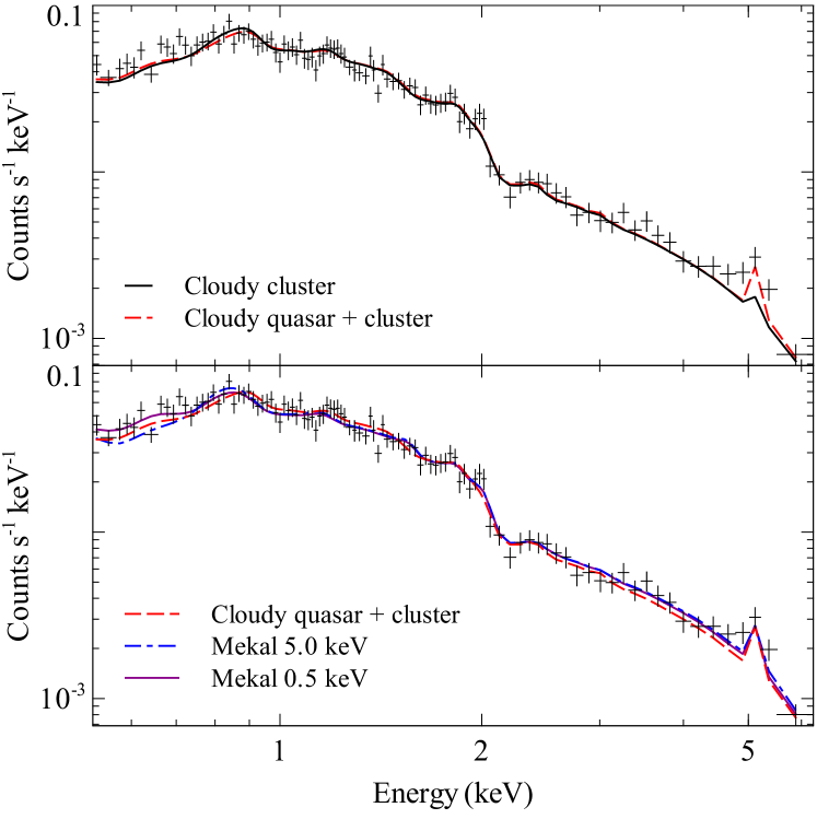
Figure 16: The cluster projected spectrum from $15-30\rm\thinspace kpc$ is shown with the best-fit Cloudy and xspec models superimposed. Upper: the Cloudy models for the cluster gas (black solid line) and the cluster gas irradiated by the quasar (red dashed line). Lower: the Cloudy model irradiated by the quasar (red dashed line) and the two-temperature mekal model with a $5.0\rm\thinspace keV$ (blue dot-dashed line) or a $0.5\rm\thinspace keV$ (purple solid line) second temperature component. The contribution of the quasar PSF was included as a phabs(powerlaw) component in each model. The three models produce a very similar spectral fit.

However, whilst our Cloudy simulations suggest that the quasar could be significantly photoionizing the gas close to the nucleus, there are several other possible explanations for the observed drop in core metallicity. Buote & Canizares (1994) argue that fitting intrinsically multitemperature spectra with single-temperature models artificially produces a lower metallicity value. There could be a significant contribution from a second temperature component in the observed projected spectrum of H1821+643, such as a hotter projected cluster emission or emission from cooling gas in the cluster core.

We therefore added a second temperature component to our xspec model to give a phabs(powerlaw)+phabs(mekal+mekal) model which was fitted to the projected spectrum ($15-30\rm\thinspace kpc$). The second temperature component was first fixed to $5.0\rm\thinspace keV$ and the metallicity in both temperature components was fixed to $0.5\hbox{$\thinspace\mathrm{Z}_{\odot}$}$. Fig. 16 (lower panel) shows that the addition of a second temperature component produced an improved fit to the Fe K $\alpha$ line blend. However, a cooler second temperature component of $0.5\rm\thinspace keV$ was found to provide a significantly better fit to the projected spectrum than the $5.0\rm\thinspace keV$ component ($\hbox{$\chi^{2}$}=94$ for $0.5\rm\thinspace keV$ compared to $\hbox{$\chi^{2}$}=109$ for $5.0\rm\thinspace keV$ with 99 degrees of freedom). Fig. 16 suggests that a second temperature component, hotter or colder, or photoionization of the cluster gas could explain the poor fit to the Fe K $\alpha$ line blend.

Assuming pressure equilibrium, the volume filling fraction of the $0.5\rm\thinspace keV$ temperature component $i$ is

$$f_{i}=\frac{\varepsilon_{i}T_{i}^{2}}{\sum_{j}\varepsilon_{j}T_{j}^{2}}$$ (6)

where $\varepsilon_{i}$ is the emission measure (xspec normalization) of the component $i$, $T_{i}$ is the temperature and $j$ sums over all the components. The $0.5\rm\thinspace keV$ temperature component has a volume filling fraction of $0.2\%$, which equates to a gas mass of $M_{gas}\sim 3\times 10^{9}\hbox{$\rm\thinspace M_{\odot}$}$. With a very short radiative gas cooling time of only $50\rm\thinspace Myr$, the $0.5\rm\thinspace keV$ temperature component could produce a mass deposition rate of $\sim 50\hbox{$\hbox{$\rm\thinspace M_{\odot}$}\rm\thinspace yr^{-1}\,$}$ in the central $30\rm\thinspace kpc$ in the absence of heating.

Finally, an additional power-law component from inverse-Compton emission could also provide an explanation for the poor fit to Fe K $\alpha$. A power-law component would raise the level of the continuum emission in the projected spectrum and reduce the prominence of the emission lines, in a similar way to the extra $5\rm\thinspace keV$ temperature component. However, coincident cluster emission and quasar PSF made it difficult to put any constraints on inverse-Compton emission and therefore we cannot determine whether this would resolve the model fit.

Although from our results it is not possible to determine a preferred explanation for the poor fit to the Fe K $\alpha$ line blend, we argue that a combination of the above would be most likely. The projected spectrum will contain a contribution of hotter ($5.0-8.0\rm\thinspace keV$) gas from the outer cluster layers. Our Cloudy simulations suggest that the quasar emission should produce a significant amount of photoionization in the central $30\rm\thinspace kpc$. Observations of strong cool-core clusters with the XMM-Newton Reflection Grating Spectrometer have confirmed that many have a second cooler temperature component in the central region (Peterson et al. 2003; Kaastra et al. 2004; Sanders et al. 2008). Finally, although we are unable to quantify any inverse-Compton emission, this could also be a factor close in to the nucleus.

6.4 AGN Unified Accretion Model

Churazov et al. (2005) (see also Di Matteo et al. 2005; Croton et al. 2006) argue that a parallel can be drawn between the evolution of Galactic black holes (eg. Fender et al. 1999; Gallo et al. 2003) and SMBHs (Merloni et al. 2003; Maccarone et al. 2003; Falcke et al. 2004; Chiaberge et al. 2005). SMBHs and their surrounding medium are therefore expected to evolve through two stages. Early on, the SMBH grows rapidly by accreting cooling gas near the Eddington rate with weak feedback on the surrounding medium but a very high radiation efficiency (eg. Yu & Tremaine 2002). This is known as the ‘quasar-mode’ which terminates when, despite the weak coupling to the gas, the SMBH produces enough heat to suppress cooling. With a lower accretion rate, the system moves to a more passively evolving stage, ‘radio-mode’, where efficient mechanical feedback sustains the ICM at X-ray temperatures. Recent observations of nearby low-luminosity SMBHs in clusters and galaxies suggest that mechanical feedback from the AGN, in the form of bubbles, shocks and sound waves, is effective at heating the cluster gas (eg. Fabian et al. 2003; Bîrzan et al. 2004; Dunn & Fabian 2006; Rafferty et al. 2006; Fabian et al. 2006).

With rapid accretion at half of the Eddington rate, H1821+643 is currently in ‘quasar-mode’, corresponding to the high/soft state of black hole X-ray binaries where a geometrically thin, optically thick accretion disk forms (Shakura & Sunyaev 1973). However, quantifying the quasar feedback into the surrounding ICM in H1821+643 is difficult. H1821+643 has a gas cooling time profile typical of a strong cool-core cluster with a passive central engine indicating that the quasar has not strongly affected the large-scale cluster gas properties. The Cloudy simulations detailed in section 6.3 also suggest that the radiative output of the luminous quasar has little impact on the bulk of the cluster gas. There is some indication of mechanical heating, although this has a low heating power and would only currently compensate for $\sim 10\%$ of the ICM cooling losses. As discussed in section 6.1, there is no obvious evidence for X-ray absorbing winds in H1821+643 in the existing observations. However, outflows might not be evident along our line of sight and therefore cannot be ruled out. Although the cluster gas properties do not indicate any efficient feedback from quasar winds on the scales considered ($r>15\rm\thinspace kpc$) this does not exclude an efficient coupling to the cold galaxy gas (see Chartas et al. 2002, 2003, 2007; Pounds et al. 2003; Reeves et al. 2009).

H1821+643 could provide an example of the early stage of evolution for these systems where the SMBH has not evolved beyond ‘quasar-mode’ and cannot produce enough heat to suppress cooling in this rich cluster. The underlying cluster may exhibit the early cool-core environment before ‘radio-mode’ heating switches on to efficiently reheat the gas. It seems implausible that the quasar could remain switched on for longer than $\sim 10^{8}\rm\thinspace yr$ because in that time the black hole mass will increase to $\sim 10^{10}\hbox{$\rm\thinspace M_{\odot}$}$, greater than the typical observed upper limit (eg. Marconi et al. 2004).

However, the FR I radio structure shown by H1821+643 appears to be at odds with the simple picture of ‘quasar-mode’ feedback. Around 10% of quasars are known to have strong radio emission (eg. Ivezić et al. 2002) indicating that SMBHs with high accretion rates can be associated with powerful outflows. By drawing comparisons with observations of microquasars, Nipoti et al. (2005) suggest a parallel between radio-loudness in quasars and the flaring mode in microquasars, where radio-loudness is simply defined as extended radio emission (FR I or FR II). Microquasars have been observed to have two distinct modes of energy output: one producing roughly steady radio emission that is coupled with X-ray emission (coupled mode), the other producing strongly variable, flaring radio emission that appears to be decoupled from the X-ray emission (flaring mode). Nipoti et al. (2005) further associate radio-quiet quasars with non-flaring/coupled states of microquasars, in either low/hard or high/soft states.

In this picture, H1821+643 would be classed as a radio-loud quasar in flaring mode, where the nucleus is producing the extended FR I radio structure. These flares could be analogous to the short, radio outbursts that have been observed in transient X-ray binaries during the transition from the low/hard to high/soft state when the accretion rate approaches the Eddington limit (Fender et al. 2004). However, whilst black hole accretion can be scaled from microquasars and X-ray binaries up to quasars, the environments of these objects vary significantly. It is unclear how the rich cluster environments and accretion history of quasars will affect the conclusions drawn from smaller scale systems.

7 Conclusions

By accurately subtracting the quasar contribution, we were able to determine the properties of the surrounding ICM down to $3\arcsec$ from the quasar. The temperature of the cluster gas decreases from $9.0\pm 0.5\rm\thinspace keV$ beyond $\sim 200\rm\thinspace kpc$ down to $1.3\pm 0.2\rm\thinspace keV$ inside $20\rm\thinspace kpc$, with a short central radiative cooling time of $1.0\pm 0.1\rm\thinspace Gyr$, typical of a strong cool-core cluster. By comparing the cooling time with a sample of cool-core clusters with ‘radio-mode’ AGN, we determined that the quasar does not appear to have had a significant impact on the large-scale cluster gas properties.

The cluster core features several extended arms of emission, which could have been dragged out by the expanding FR I structure. However, we found that the radio emission is not clearly related to the X-ray gas morphology. The nature of the surface brightness edge at $\sim 15\arcsec$ could not be unequivocably determined from the temperature and density profiles. This could be interpreted as a weak shock generated by the expansion of the radio lobes, or a cold front produced by the cool-core sloshing in the cluster’s gravitational potential. There is some evidence for cavity heating in the cluster core which could currently compensate for $\sim 10\%$ of the ICM cooling losses.

The derived accretion rate of $40\hbox{$\hbox{$\rm\thinspace M_{\odot}$}\rm\thinspace yr^{-1}\,$}$ is approximately half of the quasar’s Eddington limit. We showed that Bondi accretion, boosted by Compton cooling of the accretion material by the quasar radiation, could provide a significant proportion of the required fuel. However, without resolving the cluster gas properties at the Bondi radius, we could not determine whether this mechanism could supply all of the required $40\hbox{$\hbox{$\rm\thinspace M_{\odot}$}\rm\thinspace yr^{-1}\,$}$ and potentially provide a self-sustaining fuel source for the quasar. We have also discussed the alternative mechanisms of cold accretion or a rapid infall of a large quantity cool gas provided by a subcluster merger.

In the context of AGN unified accretion models, we suggest that H1821+643 could provide an example of the early stage of evolution for these systems where the SMBH has not evolved beyond ‘quasar-mode’ and cannot produce enough heat to suppress cooling. The surrounding rich cluster could therefore exhibit the early cool-core environment before the onset of ‘radio-mode’ heating efficiently reheats the gas. However, the powerful FR I radio structure observed in H1821+643, and in around 10% of quasars (eg. Ivezić et al. 2002), conflicts with this simple scenario of ‘quasar-mode’ feedback. Following the comparisons with observations of microquasars suggested by Nipoti et al. (2005), we consider that H1821+643 is in a flaring mode where the radio emission is decoupled from the X-ray emission. These flares could be analogous to the short, radio bursts observed in transient X-ray binaries during the transition from the low/hard to high/soft state (Fender et al. 2004). However, it is unclear how the conclusions drawn from the smaller scale systems will be affected by the rich cluster environment and the quasar accretion history.

Appendix A: Simulating the Quasar PSF

A1 Readout streak spectrum

For heavily piled up sources, M. Bautz suggested using the ACIS readout streak to extract a source spectrum (Gaetz 2004). In this observation, ACIS accumulates events for a frame exposure time of $3.1\rm\thinspace s$ and then reads out the frame at a parallel transfer rate of $40\hbox{$\mu\rm\thinspace s\,$}$, taking a total of $0.04104\rm\thinspace s$ to read out the entire frame. During readout, the CCD still accumulates events, which are distributed along the whole column as it is read out, creating a continuous streak for very bright point sources.

Figure 17: H1821+643 readout streak spectrum and spectral fit. The spectrum has been scaled by the ratio of the observation exposure time to the effective streak exposure time.

We extracted a spectrum in the energy range $0.5-7.0\rm\thinspace keV$ from two narrow regions ($300\times 8\rm\thinspace pixel^{2}$) of the readout streak positioned either side of the central source and avoiding as much of the cluster emission as possible. Any remaining cluster emission in the spectrum was then subtracted by using background regions adjacent to the readout streak. Using a wider extraction region for the readout streak was found to increase the uncertainty in the spectrum without altering the results.

The accumulated exposure time in the streak during frame transfer was $(300\times 2)\times 27463\times 40\hbox{$\mu\rm\thinspace s\,$}=659.11s$, where 27463 was the total number of frames. Therefore, the readout spectrum count rate was multiplied by a factor of 129.17, the ratio of the observation exposure time to the readout streak exposure time. Previous analyses of Chandra readout streak data have indicated that a gain correction of $+2.5\%$ for the ACIS-S3 chip (Gaetz 2004). Frame transfer is effectively a different ACIS mode for which there is likely to be a different response to arriving events compared to the calibrate timed exposure mode. However, for the H1821+643 readout streak on the ACIS-S3 chip, we found that the recommended $+2.5\%$ gain correction did not significantly alter the spectral fitting results and have not applied it to our analysis.

The response files for the transfer streak spectrum were generated using the standard ciao tools mkacisrmf and mkwarf. The response matrix (RMF) was extracted over the readout streak region used in this analysis. However, the effective area (ARF) was determined using a region at the location of the quasar image. The X-rays in the transfer streak actually hit the detector at the direct image, and their detected position is an artifact of the chip readout. The scaled readout streak spectrum was grouped with a minimum of 50 counts per spectral bin, corrected for the applied count rate scaling factor.

The scaled readout streak spectrum, shown in Fig. 17, was fitted with an absorbed power-law model in the spectral fitting package xspec version 12. The best fit photon index was consistent with the Fang et al. (2002) analysis of the Chandra HEG and MEG spectra and the previous ASCA result (Yamashita et al. 1997). Therefore, we fixed the photon index to the more accurate HEG/MEG result, $\Gamma=1.761^{+0.047}_{-0.052}$ (Fang et al. 2002). The Galactic absorption parameter was left free, giving a value of $0.003\times 10^{22}\hbox{$\rm\thinspace cm^{-2}\,$}$ with an upper limit of $0.04\times 10^{22}\hbox{$\rm\thinspace cm^{-2}\,$}$. Fang et al. (2002) inferred from the low best-fit column density $n_{\mathrm{H}}$ that H1821+643 has a soft excess. However, the best-fit absorbed powerlaw is a sufficiently good description of the readout streak spectrum so we have used this simplistic model in our analysis.

The best-fitting model gave an unabsorbed flux of $\left(1.45^{+0.04}_{-0.03}\right)\times 10^{-11}\hbox{$\rm\thinspace erg\rm\thinspace cm^{-2}\rm\thinspace s^{-1}\,$}$ in the energy range $2-10\rm\thinspace keV$ and a reduced $\chi^{2}_{\nu}=1.6$. The quasar flux measured from the readout streak spectrum falls between the values determined for this object by Fang et al. (2002) and Yamashita et al. (1997). This gives a $2-10\rm\thinspace keV$ quasar luminosity of $\left(4.2\pm 0.1\right)\times 10^{45}\hbox{$\rm\thinspace erg\rm\thinspace s^{-1}\,$}$.

This spectral model from the quasar readout streak was used as the principal component in the ChaRT simulation of the quasar.

A2 ChaRT simulations

The Chandra Ray Tracer (ChaRT), in conjunction with the marx software, was used to simulate the Chandra PSF produced by the quasar. Following the ChaRT analysis threads, the readout streak spectrum and observation exposure time were used to generate a ray-tracing simulation. The output from ChaRT was then supplied to marx version 4.4.0 which projected the ray traces onto the detector and applied the detector response.

ChaRT provides a user-friendly interface to the SAOTrace semi-empirical model (Jerius et al. 1995) which is based on the measured characteristics of the mirrors, support structures and baffles. The model is then calibrated by comparison with actual observations. However, while the PSF core and inner wing region match well with observations (Jerius 2002), the PSF wings beyond $10\arcsec$, produced by mirror scattering, seem to be underpredicted by the raytrace model. At the moment, the SAOTrace model does not model the dither motion of the telescope or include residual blur from aspect reconstruction errors. marx includes the effects of these errors using the DitherBlur parameter. We have therefore tested the use of SAOTrace to simulate the H1821+643 quasar spectra by performing an identical analysis on the quasar 3C 273, which has no surrounding cluster emission. Both of these sources are close to on-axis and only the PSF core and inner wing region are of interest to our analysis. Beyond $10\arcsec$ the cluster emission in H1821+643 will dominate and an accurate model of the quasar PSF becomes much less important.

A2.1 Test object 3C 273

3C 273 is a bright, nearby ($z=0.158$) radio-loud quasar with a jet showing superluminal motion and has been intensively studied at different wavelengths (eg. Courvoisier 1998; Soldi et al. 2008). 3C 273 was observed with Chandra ACIS-S for $160\rm\thinspace ks$ to study the bright X-ray jet in detail (Jester et al. 2006). Here we used one of the $40\rm\thinspace ks$ Chandra ACIS-S exposures of this object (obs. id 4879) to test whether a ChaRT simulation using the readout streak spectrum would recover the correct result. This observation of 3C 273 was similar to that of H1821+643, featuring a piled up point source, strong readout streak, bright PSF wings but crucially no detected extended emission (the region containing the jet was excluded). Therefore this observation of 3C 273 allowed us to test our method of determining the quasar spectrum in a series of annuli and compare the result with the observed spectra without the added complication of superimposed cluster emission.

As in section A1 for H1821+643, the readout streak spectrum was extracted using two regions of the transfer streak either side of the nucleus. The spectrum was fitted with an absorbed power-law model which provided a reasonable fit for our purposes over the required energy range, reduced $\chi^{2}_{\nu}=1.2$. This simple model gave a best-fitting photon index $\Gamma=1.64^{+0.07}_{-0.04}$, Galactic absorption upper limit of $n_{\mathrm{H}}<0.015\times 10^{22}\hbox{$\rm\thinspace cm^{-2}\,$}$ and unabsorbed flux $\left(6.5^{+0.2}_{-0.4}\right)\times 10^{-11}\hbox{$\rm\thinspace erg\rm\thinspace cm^{-2}\rm\thinspace s^{-1}\,$}$ in the $2-10\rm\thinspace keV$ energy range (Fig. 18). These parameters fall within the expected range defined by the long term variability of this source (Chernyakova et al. 2007; Soldi et al. 2008 and references therein). Although 3C 273 has also been found to have a soft excess extending up to $2\rm\thinspace keV$ (Turner et al. 1985; Staubert et al. 1992) we have ignored this for our simplistic analysis. 3C 273 has a slightly lower photon index than H1821+643 which produces a wider PSF because the PSF is energy-dependent (Figure 7).

The best-fitting model to the readout streak spectrum was used as the main input for the ChaRT simulations of 3C 273. Spectra were extracted in two annuli, excluding the readout streak, with an innermost radius of $2.5\arcsec$ outside of which pileup was determined to be negligible. The exposure time of each frame in this observation of 3C 273 was $0.4\rm\thinspace s$, compared with $3.1\rm\thinspace s$ for H1821+643, which greatly reduced the number of piled up photons. These annuli were selected to contain the required minimum of 3000 counts for a good deprojection and to cover a similar area of the PSF wings to the regions used in the analysis of H1821+643. The observed and simulated spectra were deprojected and are shown overlaid in Fig. 19. The simulated spectra were generally well-matched to the observed spectra. The mismatches can be mostly accounted for by comparison with the model of the readout streak spectrum, particularly at $\sim 3\rm\thinspace keV$ where the model was a significant overestimate. The best-fitting parameters for an absorbed power-law model fitted to the observed and simulated deprojected spectra were also found to be consistent within the errors.

A ChaRT simulation based on the readout streak spectrum was therefore expected to provide an adequate description of the quasar spectrum for the series of radial bins used in this analysis.

Figure 18: 3C 273 readout streak spectrum and spectral fit. The spectrum has been scaled by the ratio of the observation exposure time to the effective streak exposure time.

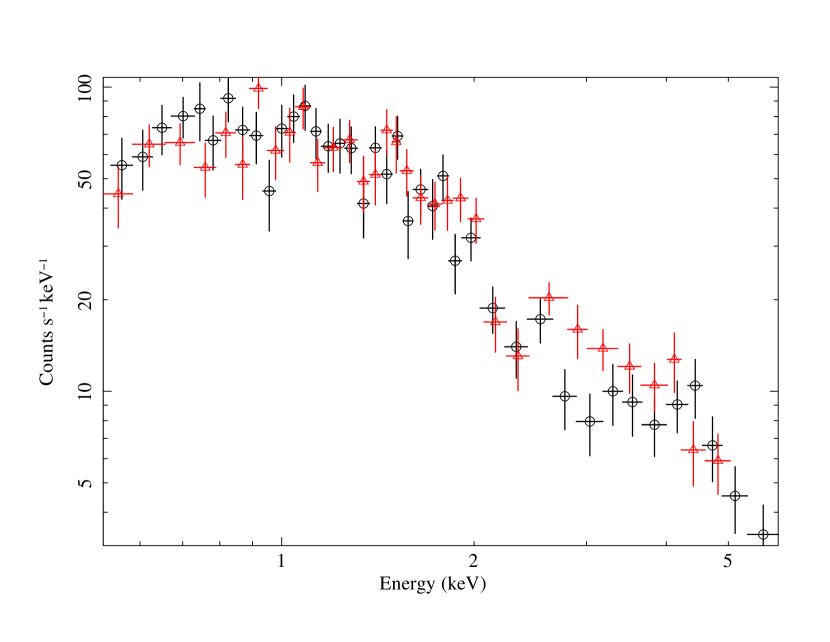
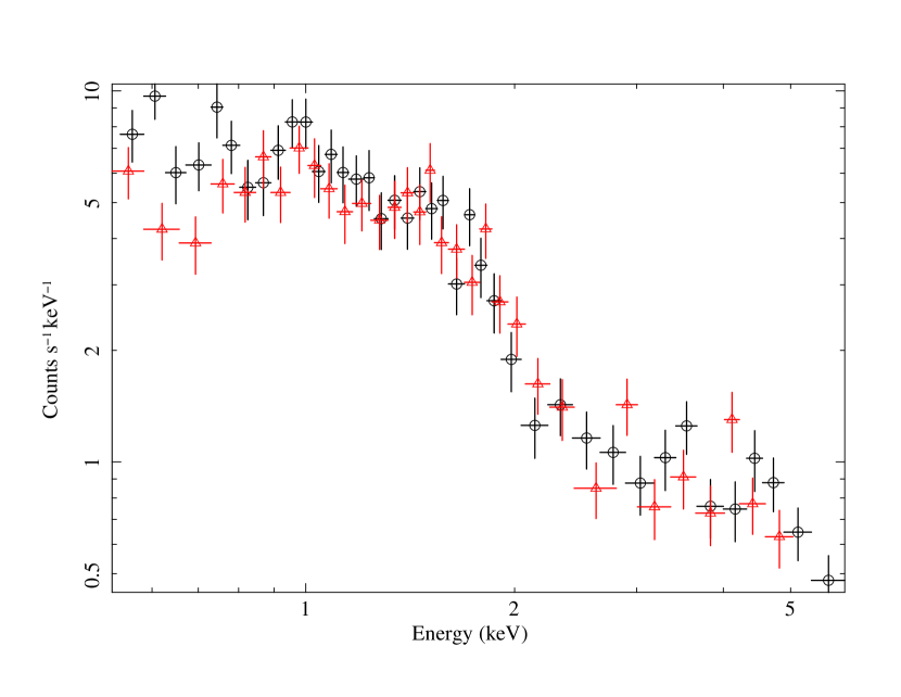
Figure 19: Comparison of the observed deprojected spectra (black circles) and ChaRT simulated deprojected spectra (red triangles) for two annuli in 3C 273. Upper: $2.5-4.9\arcsec$ Lower: $4.9-9.8\arcsec$.

A2.2 ChaRT Simulation of H1821+643

A ChaRT simulation of the quasar H1821+643 was generated for the same position on the detector using the model of the readout streak spectrum. ChaRT was run for an effective exposure time three times longer than the total observation time to sample the range of possible optical paths in the HRMA and reduce statistical errors. The raytraces were then projected onto the detector with marx to create an event file. Simulated quasar spectra were extracted from the marx event file and combined with appropriate response files for the simulation.

The width of the simulated PSF depends on the marx DitherBlur parameter, which is a statistical term combining the aspect reconstruction error, ACIS pixelization and pipeline pixel randomization. The default marx value is $0.35\arcsec$, however the magnitude of the aspect blur is observation dependent. The marx simulation of H1821+643 was repeated for DitherBlur values of $0.25\arcsec$, $0.30\arcsec$ and $0.40\arcsec$ but for all three cases the quasar-subtracted cluster surface brightness profile was consistent within statistical errors. In addition, all spectral parameters were found to be consistent within errors to the $0.35\arcsec$ simulation. We therefore proceeded with the DitherBlur parameter set to its default.

The simulated quasar spectra were extracted in identical regions to regions 1–11 (projected) and regions a–b (deprojected) shown in Fig. 5. The simulated quasar spectra from regions a–b were deprojected with dsdeproj, as detailed in section 4.3, to ensure they have been processed in an identical way to the observed deprojected spectra. By determining the quasar spectral parameters from the simulation for the same regions, we can fix these values in the combined fit to the observation of the quasar and cluster.

The simulated quasar spectrum from each region was fitted with an absorbed power-law model phabs(powerlaw) in xspec; the best-fitting parameters are given in table 1.

The difference between the best-fit n_H and power-law parameters (Table 1) and their input values from the readout streak spectrum is caused by an incorrect calculation of the effective area. This also causes the variation in these parameters between the radial bins. The effective area correction for each spectrum, provided by the ancillary response files (ARFs) assumes that all of the PSF falls within that extraction region. This was true for the cluster spectrum in each annulus but not for the quasar spectrum, where only the PSF wings were included (less than 5% of the total PSF). The effective area correction for the quasar spectrum should therefore be multiplied by the encircled energy fraction, which varies as a function of energy. When the ARF spectral response was multiplied by the EEF calculated in a series of broad energy bands from the ChaRT simulation, the input quasar parameters are recovered.

We confirmed our earlier analysis that pileup was not important beyond a radius of $3\arcsec$ from the quasar by analysing a marx simulation including pileup. The pileup simulation produced essentially identical results to the simulations without pileup and all spectral parameters were consistent within errors.

Appendix B: Cloudy Simulations

The most obvious way to model the intracluster gas using Cloudy is with the coronal equilibrium command. However, this sets up a constant temperature model which is not appropriate when we want to consider the effect of the ionizing flux from the quasar on this gas. Also, it is not clear that a pure cooling model is actually physically appropriate since the cores of clusters are known to be deficient in cool gas and this is widely thought to be due to the presence of a heat source (eg. Peterson & Fabian 2006; McNamara & Nulsen 2007). We therefore chose to model the cluster emission by using an arbitrary heat source and adjusting the heating rate to obtain the observed temperature of the cluster through a balance of heating and cooling. This was achieved using the hextra command.

Therefore, we first simulated cluster emission by creating a single zone model heated using only the hextra pure heating command. Metal abundances were set to match those measured by fitting a single temperature mekal model to the X-ray spectra, $0.4\hbox{$\thinspace\mathrm{Z}_{\odot}$}$. The heating rate was adjusted until the temperature of the gas matched that measured in the cluster in these regions ($15-30\rm\thinspace kpc$ and $22-39\rm\thinspace kpc$), $2.78\times 10^{7}\rm\thinspace K$ ($2.4\rm\thinspace keV$). This model spectrum was then renormalized to fit the cluster spectrum and the chi-square statistic evaluated. This Cloudy model for the cluster emission provided a simple comparison for the Cloudy model with the added quasar contribution; any differences could then be attributed to the quasar input and not a discrepancy between the Cloudy and mekal models of cluster emission.

To add in the quasar contribution we first generated the intrinsic continuum shape for the active nucleus using the quasar SED model described in section 6.2. To approximate the correct spectrum to irradiate the cluster gas at the distance of our extracted X-ray spectra we set up a Cloudy model with this continuum and allowed it to pass though cluster gas at a temperature of $2.78\times 10^{7}\rm\thinspace K$ ($2.4\rm\thinspace keV$) for an equivalent hydrogen column density of projected $2.3\times 10^{21}\hbox{$\rm\thinspace cm^{-2}\,$}$ ($15\rm\thinspace kpc\times 0.05\hbox{$\rm\thinspace cm^{-3}\,$}$) or deprojected $3.4\times 10^{21}\hbox{$\rm\thinspace cm^{-2}\,$}$ ($22\rm\thinspace kpc\times 0.05\hbox{$\rm\thinspace cm^{-3}\,$}$).

The transmitted spectrum from the output of this model was then added to the pure cluster simulation, allowing the hextra component to vary so that the observed temperature of the cluster was still reproduced, $2.78\times 10^{7}\rm\thinspace K$ ($2.4\rm\thinspace keV$). The emitted spectrum from this Cloudy model together with a model accounting for the quasar PSF (section 4.1) were fitted to the observed spectra from the projected ($15-30\rm\thinspace kpc$) and deprojected ($22-39\rm\thinspace kpc$) regions.

References

- Allen et al. (2006) Allen S. W., Dunn R. J. H., Fabian A. C., Taylor G. B., Reynolds C. S., 2006, MNRAS, 372, 21
- Allen et al. (2001) Allen S. W., Ettori S., Fabian A. C., 2001, MNRAS, 324, 877
- Anders & Grevesse (1989) Anders E., Grevesse N., 1989, Geochim. Cosmochim. Acta, 53, 197
- Arnaud (1996) Arnaud K. A., 1996, in Astronomical Society of the Pacific Conference Series, Vol. 101, Jacoby G. H., Barnes J., ed, Astronomical Data Analysis Software and Systems V, p. 17
- Bahcall et al. (1992) Bahcall J. N., Jannuzi B. T., Schneider D. P., Hartig G. F., Green R. F., 1992, ApJ, 397, 68
- Balucinska-Church & McCammon (1992) Balucinska-Church M., McCammon D., 1992, ApJ, 400, 699
- Bîrzan et al. (2004) Bîrzan L., Rafferty D. A., McNamara B. R., Wise M. W., Nulsen P. E. J., 2004, ApJ, 607, 800
- Blundell & Rawlings (2001) Blundell K. M., Rawlings S., 2001, ApJ, 562, L5
- Boehringer et al. (1993) Boehringer H., Voges W., Fabian A. C., Edge A. C., Neumann D. M., 1993, MNRAS, 264, L25
- Bondi (1952) Bondi H., 1952, MNRAS, 112, 195
- Buote & Canizares (1994) Buote D. A., Canizares C. R., 1994, ApJ, 427, 86
- Carter et al. (2003) Carter C., Karovska M., Jerius D., Glotfelty K., Beikman S., 2003, in Astronomical Society of the Pacific Conference Series, Vol. 295, Payne H. E., Jedrzejewski R. I., Hook R. N., ed, Astronomical Data Analysis Software and Systems XII, p. 477
- Chartas et al. (2003) Chartas G., Brandt W. N., Gallagher S. C., 2003, ApJ, 595, 85
- Chartas et al. (2002) Chartas G., Brandt W. N., Gallagher S. C., Garmire G. P., 2002, ApJ, 579, 169
- Chartas et al. (2007) Chartas G., Brandt W. N., Gallagher S. C., Proga D., 2007, AJ, 133, 1849
- Chernyakova et al. (2007) Chernyakova M. et al., 2007, A&A, 465, 147
- Chiaberge et al. (2005) Chiaberge M., Capetti A., Macchetto F. D., 2005, ApJ, 625, 716
- Churazov et al. (2005) Churazov E., Sazonov S., Sunyaev R., Forman W., Jones C., Böhringer H., 2005, MNRAS, 363, L91
- Clarke et al. (2004) Clarke T. E., Blanton E. L., Sarazin C. L., 2004, ApJ, 616, 178
- Courvoisier (1998) Courvoisier T. J.-L., 1998, A&A Rev., 9, 1
- Croton et al. (2006) Croton D. J. et al., 2006, MNRAS, 365, 11
- Davis (2001) Davis J. E., 2001, ApJ, 562, 575
- Di Matteo et al. (2005) Di Matteo T., Springel V., Hernquist L., 2005, Nat, 433, 604
- Dunn & Fabian (2004) Dunn R. J. H., Fabian A. C., 2004, MNRAS, 355, 862
- Dunn & Fabian (2006) Dunn R. J. H., Fabian A. C., 2006, MNRAS, 373, 959
- Edge & Frayer (2003) Edge A. C., Frayer D. T., 2003, ApJ, 594, L13
- Fabian (1994) Fabian A. C., 1994, ARA&A, 32, 277
- Fabian & Crawford (1990) Fabian A. C., Crawford C. S., 1990, MNRAS, 247, 439
- Fabian et al. (1981) Fabian A. C., Hu E. M., Cowie L. L., Grindlay J., 1981, ApJ, 248, 47
- Fabian et al. (2003) Fabian A. C., Sanders J. S., Allen S. W., Crawford C. S., Iwasawa K., Johnstone R. M., Schmidt R. W., Taylor G. B., 2003, MNRAS, 344, L43
- Fabian et al. (2000) Fabian A. C. et al., 2000, MNRAS, 318, L65
- Fabian et al. (2006) Fabian A. C., Sanders J. S., Taylor G. B., Allen S. W., Crawford C. S., Johnstone R. M., Iwasawa K., 2006, MNRAS, 366, 417
- Falcke et al. (2004) Falcke H., Körding E., Markoff S., 2004, A&A, 414, 895
- Fang et al. (2002) Fang T., Davis D. S., Lee J. C., Marshall H. L., Bryan G. L., Canizares C. R., 2002, ApJ, 565, 86
- Fender et al. (1999) Fender R. et al., 1999, ApJ, 519, L165
- Fender et al. (2004) Fender R. P., Belloni T. M., Gallo E., 2004, MNRAS, 355, 1105
- Ferland et al. (1998) Ferland G. J., Korista K. T., Verner D. A., Ferguson J. W., Kingdon J. B., Verner E. M., 1998, PASP, 110, 761
- Forman et al. (2005) Forman W. et al., 2005, ApJ, 635, 894
- Fried (1998) Fried J. W., 1998, A&A, 331, L73
- Gaetz (2004) Gaetz T. J., 2004, Analysis of the Chandra On-Orbit PSF Wings, http://cxc.harvard.edu/cal/Hrma/psf/
- Gallo et al. (2003) Gallo E., Fender R. P., Pooley G. G., 2003, MNRAS, 344, 60
- Hall et al. (1997) Hall P. B., Ellingson E., Green R. F., 1997, AJ, 113, 1179
- Hatch et al. (2007) Hatch N. A., Crawford C. S., Fabian A. C., 2007, MNRAS, 380, 33
- Hicks & Mushotzky (2005) Hicks A. K., Mushotzky R., 2005, ApJ, 635, L9
- Hutchings & Neff (1991) Hutchings J. B., Neff S. G., 1991, AJ, 101, 2001
- Ivezić et al. (2002) Ivezić Ž. et al., 2002, AJ, 124, 2364
- Jerius (2002) Jerius D., 2002, Comparison of on-axis Chandra Observations of AR Lac to SAOsac Simulations, http://cxc.harvard.edu/cal/Hrma/psf/ARLac-onaxis.ps
- Jerius et al. (1995) Jerius D., Freeman M., Gaetz T., Hughes J. P., Podgorski W., 1995, in Astronomical Society of the Pacific Conference Series, Vol. 77, Shaw R. A., Payne H. E., Hayes J. J. E., ed, Astronomical Data Analysis Software and Systems IV, p. 357
- Jester et al. (2006) Jester S., Harris D. E., Marshall H. L., Meisenheimer K., 2006, ApJ, 648, 900
- Johnstone et al. (1987) Johnstone R. M., Fabian A. C., Nulsen P. E. J., 1987, MNRAS, 224, 75
- Jones & De Young (2005) Jones T. W., De Young D. S., 2005, ApJ, 624, 586
- Kaastra (1992) Kaastra J. S., 1992, in Internal SRON-Leiden Report, updated version 2.0
- Kaastra et al. (2004) Kaastra J. S. et al., 2004, A&A, 413, 415
- Kalberla et al. (2005) Kalberla P. M. W., Burton W. B., Hartmann D., Arnal E. M., Bajaja E., Morras R., Pöppel W. G. L., 2005, A&A, 440, 775
- Kolman et al. (1993) Kolman M., Halpern J. P., Shrader C. R., Filippenko A. V., Fink H. H., Schaeidt S. G., 1993, ApJ, 402, 514
- Kriss et al. (1983) Kriss G. A., Cioffi D. F., Canizares C. R., 1983, ApJ, 272, 439
- Lacy et al. (1992) Lacy M., Rawlings S., Hill G. J., 1992, MNRAS, 258, 828
- Liedahl et al. (1995) Liedahl D. A., Osterheld A. L., Goldstein W. H., 1995, ApJ, 438, L115
- Maccarone et al. (2003) Maccarone T. J., Gallo E., Fender R., 2003, MNRAS, 345, L19
- Marconi et al. (2004) Marconi A., Risaliti G., Gilli R., Hunt L. K., Maiolino R., Salvati M., 2004, MNRAS, 351, 169
- Markevitch et al. (2000) Markevitch M. et al., 2000, ApJ, 541, 542
- Markevitch & Vikhlinin (2007) Markevitch M., Vikhlinin A., 2007, Phys. Rep., 443, 1
- Mathur et al. (2003) Mathur S., Weinberg D. H., Chen X., 2003, ApJ, 582, 82
- McGill et al. (2008) McGill K. L., Woo J.-H., Treu T., Malkan M. A., 2008, ApJ, 673, 703
- McNamara & Nulsen (2007) McNamara B. R., Nulsen P. E. J., 2007, ARA&A, 45, 117
- McNamara et al. (2006) McNamara B. R. et al., 2006, ApJ, 648, 164
- McNamara et al. (2000) McNamara B. R. et al., 2000, ApJ, 534, L135
- McNamara et al. (2001) McNamara B. R. et al., 2001, ApJ, 562, L149
- Merloni et al. (2003) Merloni A., Heinz S., di Matteo T., 2003, MNRAS, 345, 1057
- Mewe et al. (1985) Mewe R., Gronenschild E. H. B. M., van den Oord G. H. J., 1985, A&AS, 62, 197
- Mewe et al. (1986) Mewe R., Lemen J. R., van den Oord G. H. J., 1986, A&AS, 65, 511
- Navarro et al. (1997) Navarro J. F., Frenk C. S., White S. D. M., 1997, ApJ, 490, 493
- Nipoti et al. (2005) Nipoti C., Blundell K. M., Binney J., 2005, MNRAS, 361, 633
- O’Dea et al. (2008) O’Dea C. P. et al., 2008, ApJ, 681, 1035
- Oegerle et al. (2000) Oegerle W. R. et al., 2000, ApJ, 538, L23
- Peterson & Fabian (2006) Peterson J. R., Fabian A. C., 2006, Phys. Rep., 427, 1
- Peterson et al. (2003) Peterson J. R., Kahn S. M., Paerels F. B. S., Kaastra J. S., Tamura T., Bleeker J. A. M., Ferrigno C., Jernigan J. G., 2003, ApJ, 590, 207
- Pizzolato & Soker (2005) Pizzolato F., Soker N., 2005, ApJ, 632, 821
- Porter & Ferland (2007) Porter R. L., Ferland G. J., 2007, ApJ, 664, 586
- Pounds et al. (2003) Pounds K. A., King A. R., Page K. L., O’Brien P. T., 2003, MNRAS, 346, 1025
- Rafferty et al. (2006) Rafferty D. A., McNamara B. R., Nulsen P. E. J., Wise M. W., 2006, ApJ, 652, 216
- Reeves et al. (2009) Reeves J. N. et al., 2009, ApJ, 701, 493
- Russell et al. (2008) Russell H. R., Sanders J. S., Fabian A. C., 2008, MNRAS, 390, 1207
- Sanders (2006) Sanders J. S., 2006, MNRAS, 371, 829
- Sanders & Fabian (2007) Sanders J. S., Fabian A. C., 2007, MNRAS, 381, 1381
- Sanders et al. (2008) Sanders J. S., Fabian A. C., Allen S. W., Morris R. G., Graham J., Johnstone R. M., 2008, MNRAS, 385, 1186
- Sanders et al. (2005) Sanders J. S., Fabian A. C., Taylor G. B., 2005, MNRAS, 356, 1022
- Saxton et al. (1997) Saxton R. D., Barstow M. A., Turner M. J. L., Williams O. R., Stewart G. C., Kii T., 1997, MNRAS, 289, 196
- Schindler et al. (2001) Schindler S., Castillo-Morales A., De Filippis E., Schwope A., Wambsganss J., 2001, A&A, 376, L27
- Schmidt et al. (2001) Schmidt R. W., Allen S. W., Fabian A. C., 2001, MNRAS, 327, 1057
- Schneider et al. (1992) Schneider D. P., Bahcall J. N., Gunn J. E., Dressler A., 1992, AJ, 103, 1047
- Shakura & Sunyaev (1973) Shakura N. I., Sunyaev R. A., 1973, A&A, 24, 337
- Soldi et al. (2008) Soldi S. et al., 2008, A&A, 486, 411
- Staubert et al. (1992) Staubert R., Fink H., Courvoisier T. J.-L., Ulrich M.-H., Brunner H., Zimmermann U., Kendziorra E., Otterbein K., 1992, in American Institute of Physics Conference Series, Vol. 254, Holt S. S., Neff S. G., Urry C. M., ed, American Institute of Physics Conference Series, p. 366
- Turner et al. (1985) Turner M. J. L., Courvoisier T., Staubert R., Molteni D., Trumper J., 1985, Space Science Reviews, 40, 623
- Vasudevan & Fabian (2007) Vasudevan R. V., Fabian A. C., 2007, MNRAS, 381, 1235
- Vasudevan & Fabian (2009) Vasudevan R. V., Fabian A. C., 2009, MNRAS, 392, 1124
- Vikhlinin et al. (2001) Vikhlinin A., Markevitch M., Murray S. S., 2001, ApJ, 551, 160
- Voigt & Fabian (2006) Voigt L. M., Fabian A. C., 2006, MNRAS, 368, 518
- White et al. (1997) White D. A., Jones C., Forman W., 1997, MNRAS, 292, 419
- Yamashita et al. (1997) Yamashita A., Matsumoto C., Ishida M., Inoue H., Kii T., Makishima K., Takahashi T., Tashiro M., 1997, ApJ, 486, 763
- Yu & Tremaine (2002) Yu Q., Tremaine S., 2002, MNRAS, 335, 965